Advances in nonequilibrium transport with long-range interactions

Abstract

The effects of long-range interactions in quantum transport are still largely unexplored, mainly due to the difficulty of devising efficient embedding schemes. In this work we present a substantial progress in the interacting resonant level model by reducing the problem to the solution of Kadanoff-Baym-like equations with a correlated embedding self-energy. The method allows us to deal with short- and long-range interactions and is applicable from the transient to the steady-state regime. Furthermore, memory effects are consistently incorporated and the results are not plagued by negative densities or non-conservation of the electric charge. We employ the method to calculate densities and currents with long-range interactions appropriate to low-dimensional leads, and show the occurrence of a jamming effect which drastically reduces the screening time and suppresses the zero-bias conductance. None of these effects are captured by short-range dot-lead interactions.

Electron correlations have profound implications on the transport properties of nanoscale devicesbook . Local interactions within small molecules or quantum dots contacted to leads give rise to peculiar phenomena like Kondo effectkondo and Coulomb blockadecb , and have been the subject of several studies. Much less attention has been devoted instead to the nonlocal interactions responsible for interfacial screeening and polarization-induced renormalizations of the molecular levels. Recently, a short-range (SR) dot-lead interaction has been shown to cause a reduction of the quasiparticle gap due to the image charge effectthygesen ; thygesen2 ; bescond . In the interacting resonant level model (IRLM) the SR interaction is also at the origin of a negative differential conductance with a (interaction-dependent) power-law boulat ; nishino ; karrasch ; andergassen as well as of an overall enhancement of the off-resonance conductance bohr ; borda .

The theoretical progresses in dealing with SR dot-lead interactions are, unfortunately, not directly exportable to study long-range (LR) interactions, more appropriate for low-dimensional leads. The difficulty stems from the impossibility of combining many-body methods with embedding techniques, hence reducing the problem to the evaluation of the Green’s function of a finite and interacting open systemmeir ; jauho . Recently Elste and coworkersmillis approached the problem using the rate equations (RE) method in the IRLM with Luttinger liquid leads. The RE, however, are not reliable in the transient regime and underestimate the steady-state polarizability of the dot, as we will clearly show below. The fundamental questions which remain at present totally unanswered are therefore: What is the impact of a LR dot-lead interaction in the $I$-$V$ curve? How does the screening time change from SR to LR interactions?

In this Letter we consider the IRLM as the prototype model to address the above issues. We study the real-time evolution of the currrent and dot-density after the sudden switch-on of a bias voltage for both SR and LR dot-lead interactions. Our results indicate that LR interactions produce a jamming effect in the leads which (i) shortens the screening time and (ii) drastically suppresses the zero-bias conductance.

The proposed methodology to conclude (i) and (ii) is based on a truncation of the equations of motion for dressed correlators. The procedure leads to Kadanoff-Baym-like equations with a correlated embedding self-energy which incorporates all interaction and memory effects. Our approach overcomes the negative probability problemwhitney of the RE and is, at the same time, charge-conserving. The final equations are exact in the uncontacted case as well as in the noninteracting case and several analytic results are obtained in the steady-state, including a Meir-Wingreen-like formula for the current. We benchmarked this formula against recent results with SR interaction obtained using field theoretical methodsboulat , DMRGboulat ; bohr and other renormalization group approachborda ; karrasch ; andergassen , and found the same qualitative behavior.

We consider the IRLM described by the Hamiltonian (in standard notation)

$$H = -\sum_{\alpha}i\alpha v\int dx\,\psi^{\dagger}_{\alpha}(x)\partial_{x}\psi_{\alpha}(x)+\varepsilon_{d}n_{d}$$ (1)

$$+ \int dx\,U(x)\rho(x)n_{d}+\sum_{\alpha}\left[T_{\alpha}^{*}\psi^{\dagger}_{\alpha}(0)d+\mathrm{h.c.}\right],$$

with $\alpha=\pm 1$ for $R$ and $L$ electrons, $n_{d}=d^{\dagger}d$ and $\rho=\sum_{\alpha}\rho_{\alpha}=\sum_{\alpha}\psi^{\dagger}_{\alpha}\psi_{\alpha}$. The dot-lead interaction $U(x)$ in Eq. (1) can be either SR or LR. The system is driven out of equilibrium by the bias perturbation $H_{B}=\sum_{\alpha}V_{\alpha}\int dx\rho_{\alpha}(x)=\sum_{\alpha}V_{\alpha}N_{\alpha}$ (with $N_{\alpha}$ the number of electrons with chirality $\alpha$). For a non-perturbative treatement of the interaction we bosonize the fermion operatorsgiamarchi ; gonzbook

$$\psi_{\alpha}(x)=\frac{\eta_{\alpha}}{\sqrt{2\pi a}}e^{-2\sqrt{\pi}\,i\alpha\phi_{\alpha}(x)},$$ (2)

with boson field $\phi_{\alpha}(x)=i\alpha\sum_{q>0}\Lambda_{q}(b^{\dagger}_{\alpha q}e^{-i\alpha qx}-\mathrm{h.c.})-\frac{\sqrt{\pi}xN_{\alpha}}{\mathcal{L}}$ and $\eta_{\alpha}$ an anticommuting Klein factor. In the mode expansion of the boson field $\Lambda_{q}=\frac{e^{-\frac{aq}{2}}}{\sqrt{2\mathcal{L}q}}$, with $\mathcal{L}$ the length of the system and $a$ a short-distance cutoff. The bosonized form of the electron density takes the form $\rho_{\alpha}(x)=-\partial_{x}\phi_{\alpha}(x)/\sqrt{\pi}=\sum_{q>0}\Lambda_{q}q(b^{\dagger}_{\alpha q}e^{-i\alpha qx}-\mathrm{h.c.})+\frac{N_{\alpha}}{\mathcal{L}}$, and hence the bosonized Hamiltonian reads

$$H = \sum_{\alpha q}vqb^{\dagger}_{\alpha q}b_{\alpha q}+\varepsilon_{d}n_{d}$$ (3)

$$- \sum_{\alpha q}\frac{\Lambda_{q}q}{\sqrt{\pi}}\,U_{q}(b^{\dagger}_{\alpha q}+b_{\alpha q})n_{d}+U_{0}\sum_{\alpha}\frac{N_{\alpha}}{\mathcal{L}}n_{d}$$

$$+ \sum_{\alpha}\left[\frac{T_{\alpha}^{*}\eta^{\dagger}_{\alpha}}{\sqrt{2\pi a}}e^{-2\sqrt{\pi}\sum_{q>0}\Lambda_{q}(b^{\dagger}_{\alpha q}-b_{\alpha q})}d+\mathrm{h.c.}\right],$$

where $U_{q}=\int dx\,e^{iqx}U(x)$ and we used $U(x)=U(-x)$. Next we perform a Lang-Firsov transformation to (formally) eliminate the dot-lead coupling. The unitary operator $\mathcal{U}=e^{2\sqrt{\pi}\sum_{\alpha q}\frac{\Lambda_{q}}{2\pi v}U_{q}(b^{\dagger}_{\alpha q}-b_{\alpha q})n_{d}}$ transforms the original Hamiltonian into $\tilde{H}=\mathcal{U}^{\dagger}H\mathcal{U}$ with

$$\tilde{H} = \sum_{\alpha q}vqb^{\dagger}_{\alpha q}b_{\alpha q}+\tilde{\varepsilon}_{d}n_{d}+U_{0}\sum_{\alpha}\frac{N_{\alpha}}{\mathcal{L}}n_{d}$$ (4)

$$+ \sum_{\alpha}\left[T_{\alpha}^{*}f^{{\dagger}}_{\alpha 0}d+\mathrm{h.c.}\right]\,,\quad$$

(from now on the sum will always be over $q>0$). In the transformed Hamiltonian it appears the renormalized fermion field

$$f_{\alpha x}=\frac{\eta_{\alpha}}{\sqrt{2\pi a}}e^{2\sqrt{\pi}\sum_{\beta q}\Lambda_{q}W_{\alpha\beta q}(b^{\dagger}_{\beta q}e^{-i\alpha qx}-b_{\beta q}e^{i\alpha qx})},$$ (5)

evaluated in $x=0$, with the effective interactions $W_{RRq}=W_{LLq}=1+U_{q}/(2\pi v)$ and $W_{RLq}=W_{LRq}=U_{q}/(2\pi v)$, and the renormalized energy level $\tilde{\varepsilon}_{d}=\varepsilon_{d}+\sum_{q}\frac{e^{-aq}}{\pi v\mathcal{L}}|U_{q}|^{2}$. In the new basis the ground state of the isolated leads (i.e. for $T_{\alpha}=0$) is the vacuum $|0\rangle$ of the boson operators $b_{\alpha q}$. We can exploit this property to build the proper initial conditions by time propagation. We will consider the system initially uncontacted ($T_{\alpha}=0$), then switch on the contacts at time $t=0$ and let the current and dot-density relax. After relaxation, say at time $t_{0}$, we will bias the leads and study the screening dynamics from the transient to the steady state. This procedure simulates with high accuracy the so-called partition-free schemecini ; stef , as demonstrated in Refs. mssvl.2008 ; psc.2010 ; mcp.2011 .

We define the dot Green’s function on the Keldysh contour as

$$G(z,z^{\prime})=\frac{1}{i}\langle{\cal T}\left\{d(z)d^{{\dagger}}(z^{\prime})\right\}\rangle,$$ (6)

where ${\cal T}$ is the contour ordering, operators are in the Heisenberg picture with respect to $\tilde{H}+H_{B}$ (the bias perturbation does not change after the transformation), and the average is taken over the uncontacted ground state $|0\rangle\otimes|n\rangle$, $|n\rangle$ being the state of the dot with single ($n=1$) or zero ($n=0$) occupancy. The Green’s function obeys the equation of motion (EOM)

$$(i\partial_{z}-\tilde{\varepsilon}_{d})G(z,z^{\prime})=\delta(z,z^{\prime})+\sum_{\alpha}T_{\alpha}(z)G_{\alpha 0}(z,z^{\prime}),$$ (7)

where $G_{\alpha x}(z,z^{\prime})=\frac{1}{i}\langle{\cal T}\left\{f_{\alpha x}(z)d^{{\dagger}}(z^{\prime})\right\}\rangle$ is the dot-lead Green’s functionnote . To close the EOM we derive $G_{\alpha x}$ with respect to its first argument and find

$$\left(i\partial_{z}+i\alpha v\partial_{x}-V_{\alpha}(z)\right)G_{\alpha x}(z,z^{\prime})$$

$$=\frac{1}{i}\sum_{\beta}\langle{\cal T}\left\{\left[T^{*}_{\beta}f_{\beta 0}^{{\dagger}}d+\mathrm{h.c.},f_{\alpha x}\right](z)d^{{\dagger}}(z)\right\}\rangle.\quad\,$$ (8)

The computation of the correlator in the r.h.s. of Eq. (8) is a formidable task. In order to proceed we approximate it by $T^{*}_{\alpha}\langle\left(f_{\alpha 0}^{{\dagger}}f_{\alpha x}+f_{\alpha x}f_{\alpha 0}^{{\dagger}}\right)(z)\rangle_{P}G(z,z^{\prime})$, where $\langle\ldots\rangle_{P}$ signifies that operators are in the Heisenberg picture with respect to the uncontacted Hamiltonian. This approximation is at the basis of our truncation scheme and becomes exact in the non-interacting case as well as in the uncontacted case. Our approximation remains very accurate also for small $T_{\alpha}$ since it correctly reproduces recent results with SR dot-lead interaction (see below).

To solve the EOM for $G_{\alpha x}$ we define $g_{\alpha x\alpha x^{\prime}}(z,z^{\prime})=\frac{1}{i}\langle{\cal T}\left\{f_{\alpha x}(z)f_{\alpha x^{\prime}}^{{\dagger}}(z^{\prime})\right\}\rangle_{P}$ which satisfies the EOM

$$\left(i\partial_{z}+i\alpha v\partial_{x}-V_{\alpha}(z)\right)g_{\alpha x\alpha x^{\prime}}(z,z^{\prime})$$

$$=\delta(z,z^{\prime})\langle\left(f_{\alpha x}f_{\alpha x^{\prime}}^{{\dagger}}+f_{\alpha x^{\prime}}^{{\dagger}}f_{\alpha x}\right)(z)\rangle_{P}.$$ (9)

We can now perform a standard embedding and write the dot Green’s function as the solution of

$$(i\partial_{z}-\tilde{\varepsilon}_{d})G(z,z^{\prime})-\int_{\gamma}d\bar{z}\sum_{\alpha}\Sigma_{\alpha}(z,\bar{z})G(\bar{z},z^{\prime})=\delta(z,z^{\prime}),$$ (10)

where $\Sigma_{\alpha}(z,z^{\prime})=|T_{\alpha}|^{2}g_{\alpha 0\alpha 0}(z,z^{\prime})$ is the correlated embedding self-energy and the integral runs over the Keldysh contour. Using the Langreth ruleskeldysh Eq. (10) is converted into a coupled system of Kadanoff-Baym equations (KBE) which we solve numerically. The real-time Keldysh components of $\Sigma$ can be evaluated exactly using the bosonization methodgiamarchi ; gonzbook and read

$$\Sigma^{\lessgtr}_{\alpha}(t,t^{\prime})=\pm\frac{i|T_{\alpha}|^{2}}{2\pi a}e^{-i\varphi_{\alpha}(t)}e^{Q[\pm(t-t^{\prime})]}e^{i\varphi_{\alpha}(t^{\prime})},$$ (11)

with phase $\varphi_{\alpha}(t)=\int^{t}_{0}d\bar{t}\,V_{\alpha}(\bar{t})$ and interaction dependent exponent

$$Q(t)=\sum_{q}\frac{2\pi}{\mathcal{L}q}e^{-aq}(e^{ivqt}-1)\left[1-\frac{U_{q}}{\pi v}+\frac{1}{2}\left(\frac{U_{q}}{\pi v}\right)^{2}\right].$$ (12)

From solution of Eq. (10) we can easily calculate the dot-density from $\langle n_{d}(t)\rangle=-iG^{<}(t,t)$.

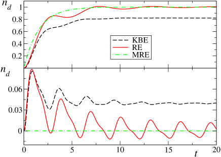
Figure 1: Time-dependent density for SR intraction using KBE (dashed), RE (solid) and MRE (dotted) for dot-energy $\tilde{\varepsilon}_{d}=0$ (top panel) and $\tilde{\varepsilon}_{d}=3$ (bottom panel) and initial dot-density $n=0$. The remaining parameters are $V_{L}=V_{R}=1$, $\gamma=0.2$, $U=0.5$, $t_{0}=0$ (partitioned scheme). Units are $10^{-1}v/a$ for $V_{\alpha}$, $\gamma$, $\tilde{\varepsilon}_{d}$, $10a/v$ for $t$ and $2\pi v$ for $U$.

Similarly, the current $I_{\alpha}$ at the interface between the dot and lead $\alpha$ can be calculate from

$$I_{\alpha}(z)=\partial_{z}N_{\alpha}(z) = -i\,T^{*}_{\alpha}\langle f^{{\dagger}}_{\alpha 0}(z)d(z)\rangle+\textrm{h.c.}$$ (13)

$$= \int_{\gamma}d\bar{z}\,\Sigma_{\alpha}(z,\bar{z})G(\bar{z},z)+\mathrm{h.c.}\quad$$

In the steady-state regime $G(t,t^{\prime})$ depends only on the time difference $t-t^{\prime}$ and the current $\bar{I}=I_{L}(t\to\infty)=-I_{R}(t\to\infty)$ is given by a Meir-Wingreen-like formula

$$\bar{I}=\int\frac{d\omega}{2\pi}\frac{\Sigma^{>}_{L}(\omega)\Sigma^{<}_{R}(\omega)-\Sigma^{<}_{L}(\omega)\Sigma^{>}_{R}(\omega)}{|\omega-\tilde{\varepsilon}_{d}-\sum_{\alpha}\Sigma_{\alpha}^{R}(\omega)|^{2}}.$$ (14)

Remarkably, the current cannot be written in terms of the difference between the leads Fermi functions despite the left and right contacts are the same.

Our analysis starts by comparing the present approximation to the RE method, recently employed in a similar contextmillis . In Fig. 1 we plot the time-dependent dot-density using the KBE, the RE and their Markovian version (MRE) for a SR interaction $U_{q}=U$. Both the KBE and RE densities exhibit oscillations with frequencies associated to charge-neutral excitations. As anticipated, however, the RE suffer from the negative-density problemwhitney (bottom panel). The MRE density is instead always non-negative but the lack of memory washes out the oscillations and the transient becomes a featureless exponential (top panel). The KBE density is superior also at the steady state. Both the RE and MRE predict a zero-temperature steady-state density either 0 or 1 and hence severely underestimate the dot polarizability. We also verified that the KBE approach is charge-conserving since fulfills with high numerical accuracy the continuity equation $d\langle n_{d}(t)\rangle/dt=I_{R}(t)+I_{L}(t)$ at every time (not shown).

We next calculate the steady-state current for a SR interaction and in the symmetric case ($\tilde{\varepsilon}_{d}=0$, $T_{L}=T_{R}=T$, $V_{L}=-V_{R}=V>0$) recently considered by several authorsboulat ; karrasch ; andergassen . In this case the integral in Eq. (14) can be performed analytically and, by defining the tunneling rate $\gamma=|T|^{2}/v$, we have

$$\bar{I}_{\mathrm{SR}}(V)\simeq\left(\frac{Va}{v}\right)^{\beta-1}\frac{\gamma}{\pi\Gamma(\beta)}\tan^{-1}\left[\frac{V}{\gamma}\left(\frac{Va}{v}\right)^{1-\beta}\Gamma(\beta)\right],$$ (15)

with exponent $\beta(U)=1+\frac{U(U-2\pi v)}{2\pi^{2}v^{2}}$. We notice that the functional form of $\bar{I}_{\mathrm{SR}}(V)$ is similar to the one derived in Ref. karrasch within functional RG, although in the present case $\beta$ is evaluated in a nonperturbative way. The above expression (plotted in Fig. 2) is also in excellent agreement with the exact results of Ref. boulat . In particular it reproduces the universal ohmic behavior $\bar{I}_{\mathrm{SR}}(V)\simeq V/\pi$ at small biasandrei (with $\sigma_{0}=1/\pi$ the quantum of conductance), and the non-universal power-law decay $\bar{I}_{\mathrm{SR}}(V)\sim V^{\beta-1}$ at large bias (the RE fail again here). The Authors of Ref. boulat observed numerically that the $\beta$-exponent does not vary monotonically with $U$, and for a special value $\bar{U}$ of the interaction reaches the maximum value $\bar{\beta}=1/2$, for which the IRLM is exactly solvable. Our formula, which is valid for all $U$, is in fair good agreement with this result, and yields $\bar{U}=\pi v$. Note also that the steady-state current is symmetric around $\bar{U}$ since $\beta(\bar{U}-\delta U)=\beta(\bar{U}+\delta U)$.

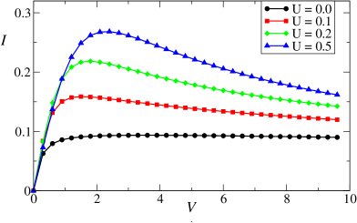
Figure 2: $I$-$V$ curve for SR interaction. The parameters are $\gamma=0.2$, $\tilde{\varepsilon}_{d}=0$. Units are $10^{-2}v/a$ for $I$, $V$, $\gamma$, $\tilde{\varepsilon}_{d}$, and $2\pi v$ for $U$.

We can now present the most important numerical results of the paper, i.e., the time-dependent current with LR interaction $U_{q}=-W\ln(aq)^{2}$. In this case the function $Q(t)$ as well as the integral in Eq. (14) must be evaluated numerically. In Fig. 3 we display the $I$-$V$ curve for several $W$’s. The behavior is qualitatively different from the SR case. In particular the zero-bias conductance is strongly suppressed with increasing $W$. Due to the LR nature of the interaction the addition/removal of an electron to/from the dot induces a charge depletion/accumulation which extends smoothly deep inside the leads (jamming effect). For a current to flow the bias must be larger than the polarization energy of this particle-hole collective state.

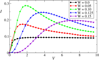
Figure 3: $I$-$V$ curve for LR interaction. Same parameters and units as in Fig. 2. $W$ is in units of $2\pi v$.

This picture also explains a common feature of the SR and LR $I$-$V$ curves, i.e., the existence of an optimal value of the interaction strenght for which the current has a maximum at fixed bias. Increasing the interaction from zero the electron density diminishes close to the dot, thus enhancing the effective tunneling rate (Coulomb deblocking). However, increasing the interaction further the particle-hole binding energy becomes larger than the charge-transfer energy $V_{L}-V_{R}$ to move an electron from one lead to the other, and the current start decreasing.

LR interactions have an impact also in the screening time. In Fig. 4 we plot the time-dependent currents for LR and SR interaction with same interaction strength $W=U$nota . The LR current relaxes faster both in the partitioned scheme (contacts and bias switched on simultaneously at $t=0$) and partition-free scheme. The same behavior is observed for different values of $W$ (not shown). The jamming effect of LR interactions is at the origin of the faster screening time. Electrons deep inside the leads suddenly respond to a change in the dot population induced by the applied bias. Finally we observe that the steady-state value of the current is the same in both schemes. This agrees with the results of Refs. stef ; mssvl.2008 ; psc.2010 ; mcp.2011 according to which the memory of the initial state is washed out in the long-time limit.

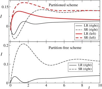
Figure 4: Time-dependent current for SR (dashed) and LR (solid) interaction for an initial density $n=0$ . The thick curves represent $I_{L}(t)$ while the thin curves $I_{R}(t)$. The parameters are $V_{L}=-V_{R}=1$, $\gamma=0.2$, $U=W=0.2$, $\bar{\varepsilon}_{d}=0$. In the top panel $t_{0}=0$ (partitioned scheme) while in the bottom panel $t_{0}=60$ (simulated partition-free scheme). Units are $10^{-1}v/a$ for $V_{\alpha}$, $\gamma$, $\tilde{\varepsilon}_{d}$, $10a/v$ for $t$ and $2\pi v$ for $U$ and $W$.

In conclusion we presented a comprehensive characterization of the transport properties of the IRLM with LR interaction. We proposed an embedding scheme based on a suitable truncation of the EOM for the dressed fermion fields and derived KBE which we solved numerically and benchmarked against available exact results. The method was compared with recently proposed RE approaches, and found to be superior from the transient (no negative densities) to the steady-state regime (no severe underestimation of the dot polarizability). LR interactions leave clear fingerprints in the time-dependent current as well as in the $I$-$V$ curve, and we believe that these features should survive when more sophisticated junctions (interacting multi-level resonant models) are considered.

References

- (1) D. V. Averin and K. K Likharev, Mesoscopic Phenomena in Solids, (Elsevier, Amsterdam, 1991).
- (2) A. C. Hewson, The Kondo Problem to Heavy Fermions (Cambridge University Press, Cambridge, 1993).
- (3) H. Grabert and M. H. Devoret, Single Charge Tunneling: Coulomb Blockade Phenomena in Nanostructures, (Plenum, New York, 1992).
- (4) K. S. Thygesen and A. Rubio, Phys. Rev. Lett. 102, 046802 (2009).
- (5) M. Strange, C. Rostgaard, H. H kkinen, and K. S. Thygesen, Phys. Rev. B 83, 115108 (2011)
- (6) Changsheng Li, M. Bescond, and M. Lannoo, Phys. Rev. B 80, 195318 (2009).
- (7) E. Boulat, H. Saleur, and P. Schmitteckert, Phys. Rev. Lett. 101, 14061 (2008).
- (8) A. Nishino, T. Imamura, and N. Hatano, Phys. Rev. Lett. 102, 146803 (2009).
- (9) C. Karrasch, M. Pletyukhov, L. Borda, and V. Meden, Phys. Rev. B 81, 125122 (2010).
- (10) S. Andergassen, M. Pletyukhov, D. Schuricht, H. Schoeller, and L. Borda, Phys. Rev. B 81, 205103 (2010).
- (11) L. Borda, K. Vladár, and A. Zawadowski, Phys. Rev. B 70, 125107 (2007).
- (12) D. Bohr and P. Schmitteckert, Phys. Rev. B 75, 241103R (2007).
- (13) Y. Meir and N. S. Wingreen, Phys. Rev. Lett. 68, 2512 (1992).
- (14) A.-P. Jauho, N. S. Wingreen, and Y. Meir, Phys. Rev. B 50, 5528 (1994).
- (15) F. Elste, D. R. Reichman, and A. J. Millis, Phys. Rev. B 83, 245405 (2011).
- (16) R. S. Whitney, J. Phys. A: Math. Theor. 41, 175304 (2008).
- (17) T. Giamarchi, Quantum Physics in One Dimension (Clarendon, Oxford, 2004).
- (18) J. Gonzàlez, M. A. Martín-Delgado, G. Sierra and M. A. H. Vozmediano, Quantum Electron Liquids and High- Superconductivity, Springer-Verlag, Berlin (1995).
- (19) M. Cini, Phys. Rev. B 22, 5887 (1980).
- (20) G. Stefanucci and C. O. Almbladh, Phys. Rev. B 69, 195318 (2004).
- (21) P. Myöhänen, A. Stan, G. Stefanucci, and R. van Leeuwen, Europhys. Lett. 84, 67001 (2008).
- (22) E. Perfetto, G. Stefanucci and M. Cini, Phys. Rev. Lett. 105, 156802 (2010).
- (23) V. Moldoveanu, H. D. Cornean and C.-A. Pillet, Phys. Rev. B 84, 075464 (2011).
- (24) The term renormalizes the energy . Indeed with the equilibrium density of lead . Since the dot induces fluctuations of order we have .
- (25) R. van Leeuwen, N. E. Dahlen, G. Stefanucci, C. O. Almbladh, and U. von Barth, Time-Dependent Density Functional Theory (Springer, New York, 2006); Lect. Notes Phys. 706, 33 (2006); M. Cini, Topics and Methods in Condensed Matter Theory (Springer-Verlag, Berlin, 2007).
- (26) P. Mehta and N. Andrei, Phys. Rev. Lett. 96, 216802 (2006).
- (27) This comparison is based on the idea of having an interaction parametrically dependent on . is SR for whereas is LR for .