The effect of edge and impurities sites properties on their localized states in semi-infinite zigzag edged 2D honeycomb graphene sheet

Maher Ahmed Department of Physics and Astronomy, University of Western Ontario, London ON N6A 3K7, Canada Physics Department, Faculty of Science, Ain Shams University, Abbsai, Cairo, Egypt mahmed62@uwo.ca
Abstract

In this work, the tridiagonal method Ahmed (2011a) is used to distinguish between edges modes and area modes to study the edge sites properties effect on edge localized states of semi-infinite zigzag 2D honeycomb graphene sheet. The results show a realistic behavior for the dependance of edge localized states of zigzag graphene on the edge sites properties which explaining the experimental results of measured local density of states at the edge of graphene Klusek et al. (2005), while at the same time removing the inconsistence between the semiconductor behavior found in the experimental data for fabricated GNRs Wang et al. (2008); Bing Huang and hui Duan (2009) and the expected theoretical semi-metallic behavior calculated without considering the edge properties effect on the edge localized states Nakada et al. (1996); Wakabayashi et al. (1999); Fujita et al. (1996); Castro Neto et al. (2009).

pacs:
Valid PACS appear here
preprint: V1

I Introduction

It is known that the 2D materials with zigzag edged nanoribbons of 2D honeycomb lattice structure has peculiar flat localized edge states at the Fermi level Ahmed (2011a); Nakada et al. (1996); Wakabayashi et al. (1999); Fujita et al. (1996); Castro Neto et al. (2009), which is a result of the zigzag geometry effect on the particles hopping flow in its edges sites.

These edge states are known to be important due to their effect on the electronic properties and as a consequence in a variety of future applications of the famous Zigzag Graphene Nanoribbons (ZGNR) Bing Huang and hui Duan (2009); Castro Neto et al. (2009). The edge localized states are, in general, dependent upon the ribbon size and purity of the sample Jia et al. (2011); Ahmed (2011a). From a theoretical point of view, the edges states depends on the probability for an electron to hop from a site in the edge to a bulk site, or to impurity site in the neighborhood. The edge atoms have a different coordination number from the bulk atoms, this leads to a different hopping parameter between the edge atoms and the bulk one. Such a difference is not usually considered in previous calculations for that ZGNR edge localized states with different approaches Nakada et al. (1996); Wakabayashi et al. (1999); Fujita et al. (1996); Castro Neto et al. (2009), these calculations show inconsistencies with experimental results for all fabricated GNRs that has semiconductor behavior Wang et al. (2008); Bing Huang and hui Duan (2009) which is a consequence of the absence of the flat edge states at Fermi level.

In Ahmed (2011b) we found that the tridiagonal method has an advantage in studying the edge properties effects on the edge localized states due to its ability to separate the edges modes from area modes in case of the 2D square lattice.

Therefore in this work, the tridiagonal method is used to study the effect of edge sites properties on the edge localized states of semi-infinite zigzag 2D honeycomb sheet as study case. The similarity between semi-infinite ZGNR and semi-infinite antiferromagnetic as both two-sublattice structure guide us to follow the tridiagonal method steps used in study the surface modes of Heisenberg antiferromagnetic De Wames and Wolfram (1969a); Filho et al. (2000a). The method allow us also to study the effect of impurities introduced substitutionally in impurities localized states of the semi infinite ZGNR.

II Theory for edge states and impurity states

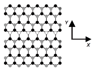
The structure of semi-infinite ZGNR is a honeycomb lattice of carbon atoms with two sublattices denoted as A𝐴A and B𝐵B. The geometry of a graphene nanoribbon with zigzag edges is shown in Figure 1, where the system is infinite in the x𝑥x direction and has 2N2𝑁2N rows of carbon atoms in the y𝑦y direction. To be considered a ribbon, N𝑁N is a finite integer but here we will extend the study for the the semi-infinite case where N𝑁N\rightarrow\infty. The A(B)𝐴𝐵A(B) sublattice type lines are labeled with index n(n)𝑛superscript𝑛n(n^{\prime}) where n(n)=1,2,3,𝑛superscript𝑛123n(n^{\prime})=1,2,3,\ldots. The impurities (which may be silicon or boron, for example) are introduced substitutionally along two different rows of atoms parallel to the x𝑥x axis. The impurity lines, which preserve the translational symmetry in the x𝑥x direction, may be any distance apart in the ribbon.
Refer to caption
Figure 1: Geometry of a graphene ribbon with zigzag edges. The black (gray) dots are the sublattice A𝐴A (B𝐵B) atoms, where A(B)𝐴𝐵A(B) sublattice type are labeled by index n(n)𝑛superscript𝑛n(n^{\prime}) (= 1,2,,N12𝑁1,2,\cdots,N) and the white dots show a row of impurities. Figure taken from Costa Filho et al. (2007).
Table 1: Nearest neighbor hopping matrix elements for the zigzag graphene nanoribbon
Parameter Zigzag
β𝛽\beta 2tcos(3qxa/2)2𝑡3subscript𝑞𝑥𝑎22t\cos(\sqrt{3}q_{x}a/2)
γ𝛾\gamma t𝑡t

Following a microscopic approach in terms of a tight binding model Hamiltonian Castro Neto et al. (2009) with neglecting the next nearest neighbor and with follow some recent work for impurities in graphene ribbons Filho et al. (2000a) the Hamiltonian becomes

H𝐻\displaystyle H =\displaystyle= i,jtij(aibj+aibj)subscript𝑖𝑗subscript𝑡𝑖𝑗subscriptsuperscript𝑎𝑖subscript𝑏𝑗subscript𝑎𝑖subscriptsuperscript𝑏𝑗\displaystyle-\sum_{i,j}t_{ij}(a^{\dagger}_{i}b_{j}+a_{i}b^{\dagger}_{j}) (1)

where aisubscriptsuperscript𝑎𝑖a^{\dagger}_{i} (or aisubscript𝑎𝑖a_{i}) creates (or annihilates) an electron on the sublattice A𝐴A site, and bjsubscriptsuperscript𝑏𝑗b^{\dagger}_{j}(or bjsubscript𝑏𝑗b_{j}) does the same for the sublattice B𝐵B site, while tijsubscript𝑡𝑖𝑗t_{ij} is the nearest-neighbor hopping energy between sublattices. In the pure material the hopping energy is denoted by t𝑡t and its value is known Castro Neto et al. (2009) to be 2.8absent2.8\approx 2.8 eV.

Taking into account the translational symmetry in x𝑥x direction, a Fourier transform is made to rewrite Equation (1) in a wavenumber representation qxsubscript𝑞𝑥q_{x} in the x𝑥x direction, and the rows are labeled n𝑛n and nsuperscript𝑛n^{\prime}. The Hamiltonian becomes

H𝐻\displaystyle H =\displaystyle= qx,nn[τ(qx)aqx,nbqx,n+τ(qx)aqx,nbqx,n].subscriptsubscript𝑞𝑥𝑛superscript𝑛delimited-[]𝜏subscript𝑞𝑥subscript𝑎subscript𝑞𝑥𝑛subscriptsuperscript𝑏subscript𝑞𝑥superscript𝑛𝜏subscript𝑞𝑥subscriptsuperscript𝑎subscript𝑞𝑥𝑛subscript𝑏subscript𝑞𝑥superscript𝑛\displaystyle\sum_{q_{x},nn^{\prime}}\left[\tau(q_{x})a_{q_{x},n}b^{\dagger}_{q_{x},n^{\prime}}+\tau(-q_{x})a^{\dagger}_{q_{x},n}b_{q_{x},n^{\prime}}\right]. (2)

The hopping amplitude factors τnn(qx)subscript𝜏𝑛superscript𝑛subscript𝑞𝑥\tau_{nn^{\prime}}(q_{x}) for the zigzag structure have the form

τnn(qx)=t[2cos(32qxa)δn,n+δn,n1],subscript𝜏𝑛superscript𝑛subscript𝑞𝑥𝑡delimited-[]232subscript𝑞𝑥𝑎subscript𝛿superscript𝑛𝑛subscript𝛿superscript𝑛minus-or-plus𝑛1\displaystyle\tau_{nn^{\prime}}(q_{x})=t\left[2\cos\left(\frac{\sqrt{3}}{2}q_{x}a\right)\delta_{n^{\prime},n}+\delta_{n^{\prime},n\mp 1}\right], (3)

or

τnn(qx)=βδn,n+γδn,n1,subscript𝜏𝑛superscript𝑛subscript𝑞𝑥𝛽subscript𝛿superscript𝑛𝑛𝛾subscript𝛿superscript𝑛minus-or-plus𝑛1\tau_{nn^{\prime}}(q_{x})=\beta\delta_{n^{\prime},n}+\gamma\delta_{n^{\prime},n\mp 1}, (4)

where the assignment of upper or lower signs depends on the sublattice type sequence for rows n𝑛n and nsuperscript𝑛n^{\prime} (see Appendix A). The definition of β𝛽\beta and γ𝛾\gamma is given Table 1. Now we use the equation of motion idX/dt=[X,H]𝑖Planck-constant-over-2-pi𝑑𝑋𝑑𝑡𝑋𝐻i\hbar dX/dt=[X,H] for any operator X𝑋X for the creation and annihilation operators of each row. Taking =1Planck-constant-over-2-pi1\hbar=1 and assuming that the modes have a time dependence like exp[iω(qx)t]𝑖𝜔subscript𝑞𝑥𝑡\exp[-i\omega(q_{x})t], we obtain 2N2𝑁2N coupled equations:

ω(qx)aqx,n𝜔subscript𝑞𝑥subscript𝑎subscript𝑞𝑥𝑛\displaystyle\omega(q_{x})a_{q_{x},n} =\displaystyle= qx,nτnn(qx)bqx,nsubscriptsubscript𝑞𝑥superscript𝑛subscript𝜏𝑛superscript𝑛subscript𝑞𝑥subscript𝑏subscript𝑞𝑥superscript𝑛\displaystyle\sum_{q_{x},n^{\prime}}\tau_{nn^{\prime}}(-q_{x})b_{q_{x},n^{\prime}}
ω(qx)bqx,n𝜔subscript𝑞𝑥subscript𝑏subscript𝑞𝑥superscript𝑛\displaystyle\omega(q_{x})b_{q_{x},n^{\prime}} =\displaystyle= qx,nτnn(qx)aqx,n.subscriptsubscript𝑞𝑥𝑛subscript𝜏superscript𝑛𝑛subscript𝑞𝑥subscript𝑎subscript𝑞𝑥superscript𝑛\displaystyle\sum_{q_{x},n}\tau_{n^{\prime}n}(q_{x})a_{q_{x},n^{\prime}}. (5)

Expanding and rearranging the Equations (5) (see Appendix A) such that coupled equations between sublattice A𝐴A and sublattice B𝐵B operators, could be written in the following form

\displaystyle- aqx,n1+{ω2(qx)(β2+γ2)}βγaqx,naqx,n+1=0subscript𝑎subscript𝑞𝑥𝑛1superscript𝜔2subscript𝑞𝑥superscript𝛽2superscript𝛾2𝛽𝛾subscript𝑎subscript𝑞𝑥𝑛subscript𝑎subscript𝑞𝑥𝑛10\displaystyle a_{q_{x},n-1}+\frac{\left\{\omega^{2}(q_{x})-\left(\beta^{2}+\gamma^{2}\right)\right\}}{\beta\gamma}a_{q_{x},n}-a_{q_{x},n+1}=0 (6)
bqx,nγω(qx)aqx,nβω(qx)aqx,n+1=0subscript𝑏subscript𝑞𝑥superscript𝑛𝛾𝜔subscript𝑞𝑥subscript𝑎subscript𝑞𝑥𝑛𝛽𝜔subscript𝑞𝑥subscript𝑎subscript𝑞𝑥𝑛10\displaystyle b_{q_{x},n^{\prime}}-\frac{\gamma}{\omega(q_{x})}a_{q_{x},n}-\frac{\beta}{\omega(q_{x})}a_{q_{x},n+1}=0

Equations (6) could be written in the following supermatrix equation De Wames and Wolfram (1969a)

(AN+ΔANONBNIN)(aNbN)=0,subscript𝐴𝑁Δsubscript𝐴𝑁subscript𝑂𝑁subscript𝐵𝑁subscript𝐼𝑁subscript𝑎𝑁subscript𝑏𝑁0\left(\begin{array}[]{cc}A_{N}+\Delta A_{N}&O_{N}\\ B_{N}&I_{N}\\ \end{array}\right)\left(\begin{array}[]{c}a_{N}\\ b_{N}\\ \end{array}\right)=0, (7)

where ONsubscript𝑂𝑁O_{N} is the null matrix, INsubscript𝐼𝑁I_{N} the identity matrix, aN(bN)subscript𝑎𝑁subscript𝑏𝑁a_{N}(b_{N}) operator column vector, and

AN=(ζ10001ζ10001ζ10001ζ1)subscript𝐴𝑁𝜁10001𝜁10001𝜁10001𝜁1A_{N}=\left(\begin{array}[]{cccccc}\zeta&-1&0&0&0&\cdots\\ -1&\zeta&-1&0&0&\cdots\\ 0&-1&\zeta&-1&0&\cdots\\ 0&0&-1&\zeta&-1&\cdots\\ \vdots&\vdots&\vdots&\vdots&\vdots&\ddots\\ \end{array}\right) (8)

and

BN=(η0000λη0000λη0000λη0),subscript𝐵𝑁𝜂0000𝜆𝜂0000𝜆𝜂0000𝜆𝜂0B_{N}=\left(\begin{array}[]{cccccc}\eta&0&0&0&0&\cdots\\ \lambda&\eta&0&0&0&\cdots\\ 0&\lambda&\eta&0&0&\cdots\\ 0&0&\lambda&\eta&0&\cdots\\ \vdots&\vdots&\vdots&\vdots&\vdots&\ddots\end{array}\right), (9)

the elements of above matrices are defined by

ζ={ω2(qx)(β2+γ2)}βγ,η=γω(qx),λ=βω(qx).formulae-sequence𝜁superscript𝜔2subscript𝑞𝑥superscript𝛽2superscript𝛾2𝛽𝛾formulae-sequence𝜂𝛾𝜔subscript𝑞𝑥𝜆𝛽𝜔subscript𝑞𝑥\displaystyle\zeta=\frac{\left\{\omega^{2}(q_{x})-\left(\beta^{2}+\gamma^{2}\right)\right\}}{\beta\gamma},\hskip 30.0pt\eta=\frac{-\gamma}{\omega(q_{x})},\hskip 30.0pt\lambda=\frac{-\beta}{\omega(q_{x})}. (10)

The edge properties have been separated from the area “bulk” properties of ZGNR by forming the matrix ΔANΔsubscript𝐴𝑁\Delta A_{N}. To simplify the calculations we consider only putting one or two impurities lines in rows numbers n0subscript𝑛0n_{0} and n0subscriptsuperscript𝑛0n^{\prime}_{0} of sublattice A𝐴A such that their properties could be separated form area properties in the same way the edge properties separated before by including them in the matrix ΔANΔsubscript𝐴𝑁\Delta A_{N}. In this case the matrix ΔANΔsubscript𝐴𝑁\Delta A_{N} has the following form

ΔAN=(ΔeΔs000000000Δs0000000000000000000000000ΔIn0000000000ΔIn0Δn0ΔIn0000000000ΔIn00000000000000000000000000ΔIn0000000000ΔIn0Δn0ΔIn0000000000ΔIn00000000000000),Δsubscript𝐴𝑁subscriptΔ𝑒subscriptΔ𝑠000000000subscriptΔ𝑠0000000000000000000000000subscriptΔ𝐼subscript𝑛0000000000subscriptΔ𝐼subscript𝑛0subscriptΔsubscript𝑛0subscriptΔ𝐼subscript𝑛0000000000subscriptΔ𝐼subscript𝑛00000000000000000000000000subscriptΔ𝐼subscriptsuperscript𝑛0000000000subscriptΔ𝐼subscriptsuperscript𝑛0subscriptΔsubscriptsuperscript𝑛0subscriptΔ𝐼subscriptsuperscript𝑛0000000000subscriptΔ𝐼subscriptsuperscript𝑛00000000000000\displaystyle\Delta A_{N}=\left(\begin{array}[]{cccccccccccc}\Delta_{e}&\Delta_{s}&0&0&0&0&0&0&0&0&0&\cdots\\ \Delta_{s}&0&0&0&0&0&0&0&0&0&0&\cdots\\ 0&0&0&0&0&0&0&0&0&0&0&\cdots\\ 0&0&0&0&\Delta_{In_{0}}&0&0&0&0&0&0&\cdots\\ 0&0&0&\Delta_{In_{0}}&\Delta_{n_{0}}&\Delta_{In_{0}}&0&0&0&0&0&\cdots\\ 0&0&0&0&\Delta_{In_{0}}&0&0&0&0&0&0&\cdots\\ 0&0&0&0&0&0&0&0&0&0&0&\cdots\\ 0&0&0&0&0&0&0&0&\Delta_{In^{\prime}_{0}}&0&0&\cdots\\ 0&0&0&0&0&0&0&\Delta_{In^{\prime}_{0}}&\Delta_{n^{\prime}_{0}}&\Delta_{In^{\prime}_{0}}&0&\cdots\\ 0&0&0&0&0&0&0&0&\Delta_{In^{\prime}_{0}}&0&0&\cdots\\ 0&0&0&0&0&0&0&0&0&0&0&\cdots\\ \vdots&\vdots&\vdots&\vdots&\vdots&\vdots&\vdots&\vdots&\vdots&\vdots&\vdots&\ddots\\ \end{array}\right), (23)

the elements of ΔANΔsubscript𝐴𝑁\Delta A_{N} matrix are defined by

ΔesubscriptΔ𝑒\displaystyle\Delta_{e} =\displaystyle= ζeζ,Δs=βγβeτeβγ,ζe={ω2(qx)(βe2+τe2)}βγ,formulae-sequencesubscript𝜁𝑒𝜁subscriptΔ𝑠𝛽𝛾subscript𝛽𝑒subscript𝜏𝑒𝛽𝛾subscript𝜁𝑒superscript𝜔2subscript𝑞𝑥superscriptsubscript𝛽𝑒2superscriptsubscript𝜏𝑒2𝛽𝛾\displaystyle\zeta_{e}-\zeta,\hskip 30.0pt\Delta_{s}=\frac{\beta\gamma-\beta_{e}\tau_{e}}{\beta\gamma},\hskip 30.0pt\zeta_{e}=\frac{\left\{\omega^{2}(q_{x})-\left(\beta_{e}^{2}+\tau_{e}^{2}\right)\right\}}{\beta\gamma},
Δn0subscriptΔsubscript𝑛0\displaystyle\Delta_{n_{0}} =\displaystyle= ζn0ζ,ΔIn0=βγβIτIβγ,ζn0={ω2(qx)(βn02+τn02)}βγ,formulae-sequencesubscript𝜁subscript𝑛0𝜁subscriptΔ𝐼subscript𝑛0𝛽𝛾subscript𝛽𝐼subscript𝜏𝐼𝛽𝛾subscript𝜁subscript𝑛0superscript𝜔2subscript𝑞𝑥superscriptsubscript𝛽subscript𝑛02superscriptsubscript𝜏subscript𝑛02𝛽𝛾\displaystyle\zeta_{n_{0}}-\zeta,\hskip 30.0pt\Delta_{In_{0}}=\frac{\beta\gamma-\beta_{I}\tau_{I}}{\beta\gamma},\hskip 30.0pt\zeta_{n_{0}}=\frac{\left\{\omega^{2}(q_{x})-\left(\beta_{n_{0}}^{2}+\tau_{n_{0}}^{2}\right)\right\}}{\beta\gamma}, (24)
Δn0subscriptΔsubscriptsuperscript𝑛0\displaystyle\Delta_{n^{\prime}_{0}} =\displaystyle= ζn0ζ,ΔIn0=βγβIn0τIn0βγ,ζn0={ω2(qx)(βn02+τn02)}βγ,formulae-sequencesubscript𝜁subscriptsuperscript𝑛0𝜁subscriptΔ𝐼subscriptsuperscript𝑛0𝛽𝛾subscript𝛽𝐼subscriptsuperscript𝑛0subscript𝜏𝐼subscriptsuperscript𝑛0𝛽𝛾subscript𝜁subscriptsuperscript𝑛0superscript𝜔2subscript𝑞𝑥superscriptsubscript𝛽subscriptsuperscript𝑛02superscriptsubscript𝜏subscriptsuperscript𝑛02𝛽𝛾\displaystyle\zeta_{n^{\prime}_{0}}-\zeta,\hskip 30.0pt\Delta_{In^{\prime}_{0}}=\frac{\beta\gamma-\beta_{In^{\prime}_{0}}\tau_{In^{\prime}_{0}}}{\beta\gamma},\hskip 30.0pt\zeta_{n^{\prime}_{0}}=\frac{\left\{\omega^{2}(q_{x})-\left(\beta_{n^{\prime}_{0}}^{2}+\tau_{n^{\prime}_{0}}^{2}\right)\right\}}{\beta\gamma},

where the edge hopping tesubscript𝑡𝑒t_{e}, the first impurities line hoping tn0subscript𝑡subscript𝑛0t_{n_{0}}, and the second impurities line hoping tn0subscript𝑡subscriptsuperscript𝑛0t_{n^{\prime}_{0}} have replaced the ZGNR interior area sites hoping t𝑡t in the definition of β𝛽\beta and γ𝛾\gamma in Table 1 to obtain the edge and impurities counterpart.

Follow the steps of Heisenberg antiferromagnetic case De Wames and Wolfram (1969a) and the algebra of block matrices Karim M. Abadir (2005), one define the supermatrix G𝐺G

G=(ANONBNIN)1=((AN)1ONBN(AN)1IN).𝐺superscriptsubscript𝐴𝑁subscript𝑂𝑁subscript𝐵𝑁subscript𝐼𝑁1superscriptsubscript𝐴𝑁1subscript𝑂𝑁subscript𝐵𝑁superscriptsubscript𝐴𝑁1subscript𝐼𝑁G=\left(\begin{array}[]{cc}A_{N}&O_{N}\\ B_{N}&I_{N}\\ \end{array}\right)^{-1}=\left(\begin{array}[]{cc}(A_{N})^{-1}&O_{N}\\ -B_{N}(A_{N})^{-1}&I_{N}\\ \end{array}\right). (25)

Multiplying Equation (25) in Equation(7), we get the following

(IN+(AN)1ΔAN)aNsubscript𝐼𝑁superscriptsubscript𝐴𝑁1Δsubscript𝐴𝑁subscript𝑎𝑁\displaystyle(I_{N}+(A_{N})^{-1}\Delta A_{N})a_{N} =\displaystyle= 00\displaystyle 0
(Bn(AN)1ΔAN)aN+bNsubscript𝐵𝑛superscriptsubscript𝐴𝑁1Δsubscript𝐴𝑁subscript𝑎𝑁subscript𝑏𝑁\displaystyle(-B_{n}(A_{N})^{-1}\Delta A_{N})a_{N}+b_{N} =\displaystyle= 00\displaystyle 0 (26)

Define the following matrix

DN=IN+(AN)1ΔANsubscript𝐷𝑁subscript𝐼𝑁superscriptsubscript𝐴𝑁1Δsubscript𝐴𝑁D_{N}=I_{N}+(A_{N})^{-1}\Delta A_{N} (27)

The matrix DNsubscript𝐷𝑁D_{N} could be written in the following partition form (see Appendix B)

DN=(QOSI),subscript𝐷𝑁𝑄𝑂missing-subexpressionmissing-subexpression𝑆𝐼D_{N}=\left(\begin{array}[]{c|c}Q&O\\ \hline\cr S&I\\ \end{array}\right), (28)

where O𝑂O is a square null matrix, I𝐼I a square identity matrix, S𝑆S a square submatrix of DNsubscript𝐷𝑁D_{N}, and Q𝑄Q is square submatrix of DNsubscript𝐷𝑁D_{N} with dimension of n0+1×n0+1subscriptsuperscript𝑛01subscriptsuperscript𝑛01n^{\prime}_{0}+1\times n^{\prime}_{0}+1.

The elements for the inverse of tridgional matrix ANsubscript𝐴𝑁A_{N} Filho et al. (2000b); Cottam and Kontos (1980); Cottam (1976); De Wames and Wolfram (1969a, b), i.e. the matrix (AN)1superscriptsubscript𝐴𝑁1(A_{N})^{-1} is given as following:

((AN)1)nm=xn+mx|nm|x+x1,subscriptsuperscriptsubscript𝐴𝑁1𝑛𝑚superscript𝑥𝑛𝑚superscript𝑥𝑛𝑚𝑥superscript𝑥1((A_{N})^{-1})_{nm}=\frac{x^{n+m}-x^{|n-m|}}{x+x^{-1}}, (29)

where x𝑥x is a complex variable such that |x|1𝑥1|x|\leq 1 and x+x1=ζ𝑥superscript𝑥1𝜁x+x^{-1}=\zeta. As mentioned in Ahmed (2011b), the values of x𝑥x should satisfy the following boundary and physical conditions Cottam and Tilley (2004). The area modes are oscillating waves inside the nanoribbon, which requires that x𝑥x must be imaginary exponential x=eiqya/2𝑥superscript𝑒𝑖subscript𝑞𝑦𝑎2x=e^{iq_{y}a/2} with |x|=1𝑥1|x|=1. From the definition of ζ𝜁\zeta and x𝑥x parameters, the dispersion relation for the area band is given by

ζ𝜁\displaystyle\zeta =\displaystyle= x+x1=eiqya/2+eiqya/2=2cos(qya/2)𝑥superscript𝑥1superscript𝑒𝑖subscript𝑞𝑦𝑎2superscript𝑒𝑖subscript𝑞𝑦𝑎22subscript𝑞𝑦𝑎2\displaystyle x+x^{-1}=e^{iq_{y}a/2}+e^{-iq_{y}a/2}=2\cos(q_{y}a/2) (30)
=\displaystyle= {ωB2(qx,qy)(β2+γ2)}βγsubscriptsuperscript𝜔2𝐵subscript𝑞𝑥subscript𝑞𝑦superscript𝛽2superscript𝛾2𝛽𝛾\displaystyle\frac{\left\{\omega^{2}_{B}(q_{x},q_{y})-\left(\beta^{2}+\gamma^{2}\right)\right\}}{\beta\gamma}
ωB(qx,qy)subscript𝜔𝐵subscript𝑞𝑥subscript𝑞𝑦\displaystyle\omega_{B}(q_{x},q_{y}) =\displaystyle= ±t1+4cos2(3qxa2)+4cos(qya2)cos(3qxa2)plus-or-minus𝑡14superscript23subscript𝑞𝑥𝑎24subscript𝑞𝑦𝑎23subscript𝑞𝑥𝑎2\displaystyle\pm t\sqrt{1+4\cos^{2}\left(\frac{\sqrt{3}q_{x}a}{2}\right)+4\cos\left(\frac{q_{y}a}{2}\right)\cos\left(\frac{\sqrt{3}q_{x}a}{2}\right)}

This expression for the 2D area band for the zigzag nanoribbons is very similar to the extended graphene electronic dispersion relation given in Castro Neto et al. (2009). This expression also shows the same general features of graphene band structure Castro Neto et al. (2009).

While the edge modes are localized on the edge and they are decaying exponentially inside the nanoribbon, which requires that x𝑥x must be real and less than 1 for edge modes. The edge modes are obtained by requiring the determinant of the coefficients for ansubscript𝑎𝑛a_{n} operator column vector to vanish De Wames and Wolfram (1969a); Cottam and Tilley (2004); Heron (1995):

|DN|=det[(QOSI)],subscript𝐷𝑁delimited-[]𝑄𝑂missing-subexpressionmissing-subexpression𝑆𝐼|D_{N}|=\det\left[\left(\begin{array}[]{c|c}Q&O\\ \hline\cr S&I\\ \end{array}\right)\right], (31)

using the rules for obtaining the determinant of partitioned matrices Karim M. Abadir (2005), Equation (31) become

|DN|=|Q||ISQ1O|=|Q|,subscript𝐷𝑁𝑄𝐼𝑆superscript𝑄1𝑂𝑄|D_{N}|=|Q||I-SQ^{-1}O|=|Q|, (32)

the localized edge and impurities states, i.e. the edge and impurities dispersion relations, for the semi-infinite zigzag are obtained by taking the limit of Equation (32) as N𝑁N\rightarrow\infty

limN|DN|=limN|Q|=|Q|.subscript𝑁subscript𝐷𝑁subscript𝑁𝑄𝑄\lim_{N\rightarrow\infty}|D_{N}|=\lim_{N\rightarrow\infty}|Q|=|Q|. (33)

In the case of taking only the edge properties effect on the edge localized states, i.e there is no any impurities lines inside the sheet, Equation (33) become

det(Q)=|A111Δe+A121Δs+1A111ΔsA211Δe+A221ΔsA211Δs+1|=0,𝑄subscriptsuperscript𝐴111subscriptΔ𝑒subscriptsuperscript𝐴112subscriptΔ𝑠1subscriptsuperscript𝐴111subscriptΔ𝑠subscriptsuperscript𝐴121subscriptΔ𝑒subscriptsuperscript𝐴122subscriptΔ𝑠subscriptsuperscript𝐴121subscriptΔ𝑠10\det(Q)=\left|\begin{array}[]{cc}A^{-1}_{11}\Delta_{e}+A^{-1}_{12}\Delta_{s}+1&A^{-1}_{11}\Delta_{s}\\ A^{-1}_{21}\Delta_{e}+A^{-1}_{22}\Delta_{s}&A^{-1}_{21}\Delta_{s}+1\\ \end{array}\right|=0, (34)

which give

Δs2x52Δsx4(2Δs2+Δe)x3(12Δs)x2+(Δs2+Δe)x1=0.superscriptsubscriptΔ𝑠2superscript𝑥52subscriptΔ𝑠superscript𝑥42superscriptsubscriptΔ𝑠2subscriptΔ𝑒superscript𝑥312subscriptΔ𝑠superscript𝑥2superscriptsubscriptΔ𝑠2subscriptΔ𝑒𝑥10\Delta_{s}^{2}x^{5}-2\Delta_{s}x^{4}-(2\Delta_{s}^{2}+\Delta_{e})x^{3}-(1-2\Delta_{s})x^{2}+(\Delta_{s}^{2}+\Delta_{e})x-1=0. (35)

In case the interaction of the edge with the interior sites is not affected with the edge sites properties, i.e. Δs=0subscriptΔ𝑠0\Delta_{s}=0, Equation (33) become

det(A)=|A111Δe+10A211Δe1|=A111Δe+1=0𝐴subscriptsuperscript𝐴111subscriptΔ𝑒10subscriptsuperscript𝐴121subscriptΔ𝑒1subscriptsuperscript𝐴111subscriptΔ𝑒10\det(A)=\left|\begin{array}[]{cc}A^{-1}_{11}\Delta_{e}+1&0\\ A^{-1}_{21}\Delta_{e}&1\\ \end{array}\right|=A^{-1}_{11}\Delta_{e}+1=0 (36)

which is the same expression obtained for Heisenberg antiferromagnetic De Wames and Wolfram (1969a).
Refer to caption
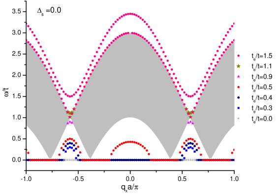
Figure 2: Edge localized states for edge with different edge hopping calculated with Δs=0subscriptΔ𝑠0\Delta_{s}=0, the shaded band represent area modes continuum.
Refer to caption
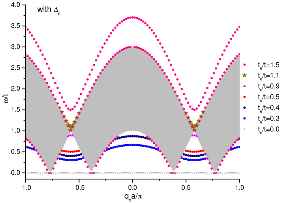
Figure 3: Edge localized states for edge with different edge hopping calculated with Δs0subscriptΔ𝑠0\Delta_{s}\neq 0, the shaded band represent area modes continuum.

III Results

Figures 3 and 3 show the edge localized states of semi-infinite zigzag graphene sheet for different edge hopping to area hopping ratios calculated with Δs=0subscriptΔ𝑠0\Delta_{s}=0 using Equation 36 for Figure 3 and calculated with Δs0subscriptΔ𝑠0\Delta_{s}\neq 0 using Equation 34 for Figure 3. The Figures show that the dispersion of the edge localized states depends on both the edge sites hopping properties and their effect on the interaction with the interior sites in the zigzag sheet.

The Figures begin with edge hopping equal to zero, which could be done by saturating the carbons atoms on the edge. In this hopping value both calculations (with and without ΔssubscriptΔ𝑠\Delta_{s}) result in an extended flat localized edge state through the whole Brilloin zone at Fermi level ωF/t=0subscript𝜔𝐹𝑡0\omega_{F}/t=0. This is due to the localized edge wave functions which agree with density-functional theory (DFT) calculations for finite ribbon Xu et al. (2010).

As the edge hopping increases from zero, the dispersion of the edge localized state begin to have a percentage of it laying at Fermi level ωF=0subscript𝜔𝐹0\omega_{F}=0, and the remaining percentage liftoff from the Fermi level. The percentage of the edge dispersion that laying at Fermi level is important to the electronic properties of the zigzag edged graphene nanoribbon.
Refer to caption Refer to caption
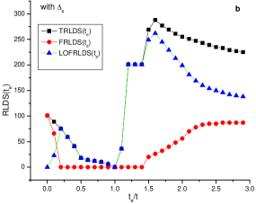
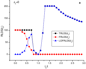
Figure 4: The variation of TRLDOS, FRLDOS, and LOFRLDOS as a function of edge hopping form 0 to 2.9. (a) for Δs=0subscriptΔ𝑠0\Delta_{s}=0 and (b) for Δs0subscriptΔ𝑠0\Delta_{s}\neq 0.

To study the variation of the edge dispersions percentage laying at Fermi level with the changing of the edge hopping and in the same time to easily clarify the data displayed in Figures 3 and 3, we define the following three parameters for each given edge hopping value. The first one is the Relative Localized Density of States near Fermi level (FRLDOS), which is calculated computationally by counting the total number of points in the localized edge dispersion with ω/t<0.2𝜔𝑡0.2\omega/t<0.2. The second parameter is the Total Relative Localized Density of States (TRLDOS), which is calculated computationally by counting the total number of points in the localized edge dispersion, which is a relative measure of its total density of states. The third parameter is the difference between FRLDOS and TRLDOS which represent the liftoff percentage of the edge localized state dispersion from Fermi level (LOFRLDOS).

Figure 4 shows the variation of TRLDOS, FRLDOS, and LOFRLDOS for edge localized states as a function of edge to area hopping ratio form 0 to 2.9 with increment of 0.1, the (a) sub Figure represent the calculation with Δs=0subscriptΔ𝑠0\Delta_{s}=0, while (b) sub Figure represent the calculation with Δs0subscriptΔ𝑠0\Delta_{s}\neq 0.

With the help of the comparison between Figure 4(a) and Figure 3 and the comparison between Figure 4(b) and Figure 3, the variation of the edge localized states dispersion with different edge hopping values is described as follow:

First, for the dispersion of localized edge state calculated using Δs=0subscriptΔ𝑠0\Delta_{s}=0, starting with edge hopping equal to zero the Figure 4(a) shows that FRLDOS is equal to TRLDOS which means that the edge localized state lays completely in the Fermi level while LOFRLDOS is zero. In Figure 3 it is shown as a flat localized edge state at Fermi level ωF/t=0subscript𝜔𝐹𝑡0\omega_{F}/t=0 extended through the whole Brilloin zone as described above. For 2 increment in the edge hopping there is no change in the value of FRLDOS and it is still equal to TRLDOS with LOFRLDOS is equal to zero, which mean that dispersion did not change from as zero hopping. Beginning from edge hopping equal to 0.3 the value of FRLDOS begin to decrease and LOFRLDOS begin to increase while TRLDOS keep constant which means that some of dispersion left off from Fermi level as shown in Figure 3 as a left off near qxa/π=±0.5subscript𝑞𝑥𝑎𝜋plus-or-minus0.5q_{x}a/\pi=\pm 0.5. As edge hopping reach 0.5 the TRLDOS still keep constant while FRLDOS still decreasing and LOFRLDOS still increases which means that more dispersion left off from Fermi level as shown in Figure 3 as increase in the left off near qxa/π=±0.5subscript𝑞𝑥𝑎𝜋plus-or-minus0.5q_{x}a/\pi=\pm 0.5 and around qxa/π=±0.0subscript𝑞𝑥𝑎𝜋plus-or-minus0.0q_{x}a/\pi=\pm 0.0. At edge hopping 0.8 the TRLDOS drop quickly to small value and it is equal to LOFRLDOS while FRLDOS become zero which means that most the edge localized dispersion disappear which shown in edge hopping 0.9 in Figure 3 as small edge localized points near the intersection of the area band segments. When edge hopping is equal to interior hopping, the edge localized states completely disappear. Figure 4(a) shows that FRLDOS is equal to zero in edge hopping range 0.92.90.92.90.9-2.9. As the edge hopping increases from 1 to 2.9, LOFRLDOS is equal to TRLDOS. The LOFRLDOS increases very quickly to large value with increasing of edge hopping from 1 to 1.3, and then keep constant in the edge hopping range 1.31.71.31.71.3-1.7 after that range LOFRLDOS decrease slowly. This behavior is shown in Figure 3 as increasing in the edge localized states above the area band.

In the second case, the dispersion of localized edge state calculated using Δs0subscriptΔ𝑠0\Delta_{s}\neq 0, starting with edge hopping equal to zero the Figure 4(b) shows that FRLDOS is equal to TRLDOS which means that the edge localized state lays completely in the Fermi level while LOFRLDOS is zero, in Figure 3 it is shown as a flat localized edge state at Fermi level ωF/t=0subscript𝜔𝐹𝑡0\omega_{F}/t=0 extended through the whole Brilloin zone as described above. At the edge hopping equal to 0.1 the values of FRLDOS and TRLDOS begin to decrease and LOFRLDOS begin to increase which means that some of dispersion left off from Fermi level. In the edge hopping range from 0.2 to 1.4, the FRLDOS become zero and TRLDOS become equal to LOFRLDOS. In edge hopping range 0.2 to 1, the LOFRLDOS decreases to a zero value, which is shown in Figure 3 as decreasing in the edge localized states dispersion, and at the same time the edge localized state shifting up in the energy. It is very important to note that at edge hopping 0.5, the edge localized states dispersion become very similar to the famous peculiar edge localized state for graphene zigzag nanoribbon Nakada et al. (1996); Wakabayashi et al. (1999); Fujita et al. (1996); Castro Neto et al. (2009) but here shifted from Fermi level due to the edge hopping properties. When edge hopping is equal to interior hopping, the edge localized states completely disappear. The LOFRLDOS increases very quickly to large value with increasing of edge hopping from 1 to 1.2, and then remains constant in the edge hopping range 1.21.41.21.41.2-1.4. After that range, the LOFRLDOS increase to a peak at edge hopping 1.6 and then it begins to slowly decrease until edge hopping 2.92.92.9. Starting from the edge hopping 1.4, the LOFRLDOS begins to slowly increase with increasing the edge hopping until the edge hopping reach 2.3, then the LOFRLDOS begins converge to a nearly constant value. While the TRLDOS increase to a peak at edge hopping 1.6 and it then begins to slowly decrease with increasing the edge hopping. The behavior of the three parameters is displayed in Figure 3 as a change in the edge localized states around the area band.
Refer to caption Refer to caption
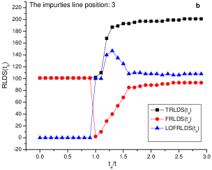
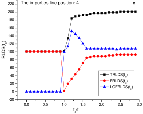
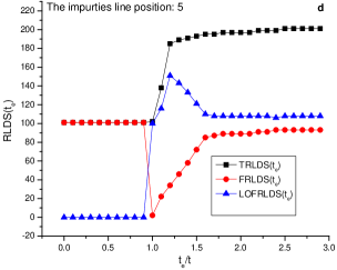
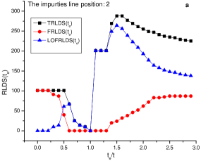
Figure 5: The variation of TRLDOS, FRLDOS, and LOFRLDOS as a function of impurities hopping form 0 to 2.9 for the impurities line in sublattice A𝐴A at positions (a) 2, (b) 3, (c) 4, (d) 5.

The effects of both the impurities hopping and the impurities line position on the impurities localized states have been calculated using Equation 33 and the results are shown in Figures 5. This calculation was done considering the edge hopping is equal to 1.

Figures 5 show the variation of TRLDOS, FRLDOS, and LOFRLDOS as a function of impurities hopping form 0 to 2.9 for the impurities line in sublattice A𝐴A at positions (a) 2, (b) 3, (c) 4, (d)5. It is clear that the dispersion of the impurities localized states for impurities line at second raw of the sublattice A𝐴A is very similar to the dispersion of the edge localized states described above. Beginning from position three in the sublattice A𝐴A, the dispersion of the impurities localized states becomes completely different and nearly independent on the impurities line position in the sublattice A𝐴A.

Figures 5(a), (b), and (c) show that for the impurities hopping range form 0 to 0.9 the FRLDOS is equal to TRLDOS which means that the impurities localized state lays completely in the Fermi level while LOFRLDOS is zero. In Figure 3 it is shown as a flat localized edge state at Fermi level ωF/t=0subscript𝜔𝐹𝑡0\omega_{F}/t=0 extended through the whole Brilloin zone as described above. At the impurities hopping equal to 1 the FRLDOS switches to zero while LOFRLDOS changes to the value that keeps TRLDOS constant. This means that the impurities localized state is completely lay off from Fermi level with keeping its density of states constant. As impurities hopping from 1 to 1.3 the LOFRLDOS rapidly increases to a peak in its value, it then decreases until the impurities hopping reach 1.7 then the LOFRLDOS begin converging to nearly a constant value. Likewise, as impurities hopping from 1 to 1.7 the FRLDOS increase until the impurities hopping reach 1.7 the FRLDOS begin converging to nearly a constant value lower that LOFRLDOS value. While the TRLDOS has fast increases in edge hopping range from 1 to 1.3 and then it begin converging to a nearly high constant value.
Refer to caption
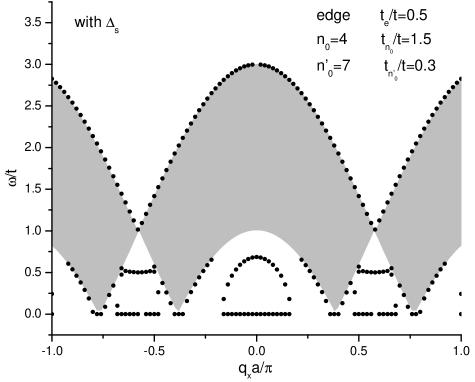
Figure 6: Edge and impurities localized states the black dots for edge and two lines of impurities at sublattice A𝐴A, the shaded band represent area modes continuum. The Edge hopping is te/t=0.5subscript𝑡𝑒𝑡0.5t_{e}/t=0.5, the first impurities line position is n0=4subscript𝑛04n_{0}=4 with impurities hopping tn0/t=1.5subscript𝑡subscript𝑛0𝑡1.5t_{n_{0}}/t=1.5, and the second impurities line position is n0=7subscriptsuperscript𝑛07n^{\prime}_{0}=7 with impurities hopping tn0/t=0.3subscript𝑡subscriptsuperscript𝑛0𝑡0.3t_{n^{\prime}_{0}}/t=0.3.

IV Discussion and Conclusions

In this work the tridiagonal method was used to study the effect of edge and impurities sites properties on their localized states in semi-infinite zigzag edged 2D honeycomb sheet. It is found that the tridiagonal method calculations provide us with two possibility to study the effect of the edges sites properties on their localized states. In the first one, the interaction of the edge with the interior sites is not affected with the edge sites properties, i.e. Δs=0subscriptΔ𝑠0\Delta_{s}=0, and in the second one the interaction of the edge with the interior sites is affected by the edge sites properties, i.e. Δs0subscriptΔ𝑠0\Delta_{s}\neq 0.

The results of the case Δs=0subscriptΔ𝑠0\Delta_{s}=0 show that the edge localized states dispersion has qxsubscript𝑞𝑥q_{x} dependance of the hopping in 1D chain Altland and Simons (2010) in low edge hopping values, which reflect the completely isolation of edge hopping from interior one. This behavior is away from the expected behavior from tight binding model results and the explanation given in Ahmed (2011a).

The results of the case Δs0subscriptΔ𝑠0\Delta_{s}\neq 0 show that the edge localized states dispersion has qxsubscript𝑞𝑥q_{x} dependance of the hopping in 2D honeycomb but shifted in the energy due to the edge hopping properties and especially at edge hopping 0.5, the edge localized states dispersion become very similar to the famous peculiar edge localized state for graphene zigzag nanoribbon Nakada et al. (1996); Wakabayashi et al. (1999); Fujita et al. (1996); Castro Neto et al. (2009) but here shifted from Fermi level. which reflect the importance of edge sites properties on the edge hopping with interior sites. In this case the behavior is agree with the expected behavior from tight binding model results and the explanation given in Ahmed (2011a).

In case of the effects of both the impurities hopping and the impurities line position on the impurities localized states, the results show that second raw of the sublattice A𝐴A has very similar edge localized states dispersion, and after that position the impurities localized states become nearly independent on the impurities line position in sublattice A𝐴A. Also, the results show that introducing impurities in any position of the sheet will produce impurities localized states at Fermi level in all impurities hopping properties, which affecting the electronic properties of the sheet.

The model could be used to study the effects of hopping properties interaction for the edge and the two separated lines of impurities at sublattice A𝐴A in the edge and the impurities localized states as shown in Figure 6.

The equivalent between the obtained mathematical expressions for edge states in case of zigzag graphene and that obtained for surface spin wave in case of Heisenberg antiferromagnetic De Wames and Wolfram (1969a) reflect their equivalent from geometrical and topological point of view. In the same time it show that result is applicable to the magnetic and the 2D materials have the same geometrical and topological structure.

Finally, the results of considering the interaction of the edge with the interior sites is affected by the edge sites properties, i.e. Δs0subscriptΔ𝑠0\Delta_{s}\neq 0, show a realistic behavior for the dependance of edge localized states of zigzag graphene on the edge sites properties which explaining the experimental results of measured local density of states at the edge of graphene Klusek et al. (2005), and in the same time removing the inconsistence between the semiconductor behavior found in the experimental data for fabricated GNRs Wang et al. (2008); Bing Huang and hui Duan (2009) and the expected theoretical semi-metallic behavior calculated without considering the edge properties effect on the edge localized states Nakada et al. (1996); Wakabayashi et al. (1999); Fujita et al. (1996); Castro Neto et al. (2009).

Acknowledgements.
This research has been supported by the Egyptian Ministry of Higher Education and Scientific Research (MZA).

References

Appendix A Rearranging Equations (5)

In this appendix we list the rearrange steps of Equations (5) to obtain Equations (6).

ω(qx)aqx,n𝜔subscript𝑞𝑥subscript𝑎subscript𝑞𝑥𝑛\displaystyle\omega(q_{x})a_{q_{x},n} =\displaystyle= qx,nτnn(qx)bqx,nsubscriptsubscript𝑞𝑥superscript𝑛subscript𝜏𝑛superscript𝑛subscript𝑞𝑥subscript𝑏subscript𝑞𝑥superscript𝑛\displaystyle\sum_{q_{x},n^{\prime}}\tau_{nn^{\prime}}(-q_{x})b_{q_{x},n^{\prime}}
ω(qx)bqx,n𝜔subscript𝑞𝑥subscript𝑏subscript𝑞𝑥superscript𝑛\displaystyle\omega(q_{x})b_{q_{x},n^{\prime}} =\displaystyle= qx,nτnn(qx)aqx,n.subscriptsubscript𝑞𝑥𝑛subscript𝜏superscript𝑛𝑛subscript𝑞𝑥subscript𝑎subscript𝑞𝑥superscript𝑛\displaystyle\sum_{q_{x},n}\tau_{n^{\prime}n}(q_{x})a_{q_{x},n^{\prime}}.

Expanding Equations (5) using the sublattice indexes n𝑛n and nsuperscript𝑛n^{\prime}

ω(qx)aqx,1𝜔subscript𝑞𝑥subscript𝑎subscript𝑞𝑥1\displaystyle\omega(q_{x})a_{q_{x},1} =\displaystyle= βbqx,1𝛽subscript𝑏subscript𝑞𝑥1\displaystyle\beta b_{q_{x},1}
ω(qx)aqx,2𝜔subscript𝑞𝑥subscript𝑎subscript𝑞𝑥2\displaystyle\omega(q_{x})a_{q_{x},2} =\displaystyle= γbqx,1+βbqx,2𝛾subscript𝑏subscript𝑞𝑥1𝛽subscript𝑏subscript𝑞𝑥2\displaystyle\gamma b_{q_{x},1}+\beta b_{q_{x},2}
ω(qx)aqx,3𝜔subscript𝑞𝑥subscript𝑎subscript𝑞𝑥3\displaystyle\omega(q_{x})a_{q_{x},3} =\displaystyle= γbqx,2+βbqx,3𝛾subscript𝑏subscript𝑞𝑥2𝛽subscript𝑏subscript𝑞𝑥3\displaystyle\gamma b_{q_{x},2}+\beta b_{q_{x},3}
\displaystyle\vdots
ω(qx)aqx,n𝜔subscript𝑞𝑥subscript𝑎subscript𝑞𝑥𝑛\displaystyle\omega(q_{x})a_{q_{x},n} =\displaystyle= γbqx,n1+βbqx,n𝛾subscript𝑏subscript𝑞𝑥superscript𝑛1𝛽subscript𝑏subscript𝑞𝑥superscript𝑛\displaystyle\gamma b_{q_{x},n^{\prime}-1}+\beta b_{q_{x},n^{\prime}}
ω(qx)bqx,1𝜔subscript𝑞𝑥subscript𝑏subscript𝑞𝑥1\displaystyle\omega(q_{x})b_{q_{x},1} =\displaystyle= βaqx,1+γaqx,2𝛽subscript𝑎subscript𝑞𝑥1𝛾subscript𝑎subscript𝑞𝑥2\displaystyle\beta a_{q_{x},1}+\gamma a_{q_{x},2}
ω(qx)bqx,2𝜔subscript𝑞𝑥subscript𝑏subscript𝑞𝑥2\displaystyle\omega(q_{x})b_{q_{x},2} =\displaystyle= βaqx,2+γaqx,3𝛽subscript𝑎subscript𝑞𝑥2𝛾subscript𝑎subscript𝑞𝑥3\displaystyle\beta a_{q_{x},2}+\gamma a_{q_{x},3}
ω(qx)bqx,3𝜔subscript𝑞𝑥subscript𝑏subscript𝑞𝑥3\displaystyle\omega(q_{x})b_{q_{x},3} =\displaystyle= βaqx,3+γaqx,4𝛽subscript𝑎subscript𝑞𝑥3𝛾subscript𝑎subscript𝑞𝑥4\displaystyle\beta a_{q_{x},3}+\gamma a_{q_{x},4}
\displaystyle\vdots
ω(qx)bqx,n𝜔subscript𝑞𝑥subscript𝑏subscript𝑞𝑥superscript𝑛\displaystyle\omega(q_{x})b_{q_{x},n^{\prime}} =\displaystyle= βaqx,n+γaqx,n+1𝛽subscript𝑎subscript𝑞𝑥𝑛𝛾subscript𝑎subscript𝑞𝑥𝑛1\displaystyle\beta a_{q_{x},n}+\gamma a_{q_{x},n+1}

divide by ω(qx)𝜔subscript𝑞𝑥\omega(q_{x}), and rearrange we get

bqx,nγω(qx)aqx,nβω(qx)aqx,n+1=0subscript𝑏subscript𝑞𝑥superscript𝑛𝛾𝜔subscript𝑞𝑥subscript𝑎subscript𝑞𝑥𝑛𝛽𝜔subscript𝑞𝑥subscript𝑎subscript𝑞𝑥𝑛10b_{q_{x},n^{\prime}}-\frac{\gamma}{\omega(q_{x})}a_{q_{x},n}-\frac{\beta}{\omega(q_{x})}a_{q_{x},n+1}=0
ω(qx)bqx,n𝜔subscript𝑞𝑥subscript𝑏subscript𝑞𝑥superscript𝑛\displaystyle\omega(q_{x})b_{q_{x},n^{\prime}} =\displaystyle= βaqx,n+γaqx,n+1𝛽subscript𝑎subscript𝑞𝑥𝑛𝛾subscript𝑎subscript𝑞𝑥𝑛1\displaystyle\beta a_{q_{x},n}+\gamma a_{q_{x},n+1}
ω(qx)bqx,n1𝜔subscript𝑞𝑥subscript𝑏subscript𝑞𝑥superscript𝑛1\displaystyle\omega(q_{x})b_{q_{x},n^{\prime}-1} =\displaystyle= βaqx,n1+γaqx,n𝛽subscript𝑎subscript𝑞𝑥𝑛1𝛾subscript𝑎subscript𝑞𝑥𝑛\displaystyle\beta a_{q_{x},n-1}+\gamma a_{q_{x},n}
ω(qx)aqx,n𝜔subscript𝑞𝑥subscript𝑎subscript𝑞𝑥𝑛\displaystyle\omega(q_{x})a_{q_{x},n} =\displaystyle= γbqx,n1+βbqx,n𝛾subscript𝑏subscript𝑞𝑥superscript𝑛1𝛽subscript𝑏subscript𝑞𝑥superscript𝑛\displaystyle\gamma b_{q_{x},n^{\prime}-1}+\beta b_{q_{x},n^{\prime}}
ω(qx)aqx,n𝜔subscript𝑞𝑥subscript𝑎subscript𝑞𝑥𝑛\displaystyle\omega(q_{x})a_{q_{x},n} =\displaystyle= γβaqx,n1+γaqx,nω(qx)+ββaqx,n+γaqx,n+1ω(qx)𝛾𝛽subscript𝑎subscript𝑞𝑥𝑛1𝛾subscript𝑎subscript𝑞𝑥𝑛𝜔subscript𝑞𝑥𝛽𝛽subscript𝑎subscript𝑞𝑥𝑛𝛾subscript𝑎subscript𝑞𝑥𝑛1𝜔subscript𝑞𝑥\displaystyle\gamma\frac{\beta a_{q_{x},n-1}+\gamma a_{q_{x},n}}{\omega(q_{x})}+\beta\frac{\beta a_{q_{x},n}+\gamma a_{q_{x},n+1}}{\omega(q_{x})}
ω2(qx)aqx,nsuperscript𝜔2subscript𝑞𝑥subscript𝑎subscript𝑞𝑥𝑛\displaystyle\omega^{2}(q_{x})a_{q_{x},n} =\displaystyle= γ(βaqx,n1+γaqx,n)+β(βaqx,n+γaqx,n+1)𝛾𝛽subscript𝑎subscript𝑞𝑥𝑛1𝛾subscript𝑎subscript𝑞𝑥𝑛𝛽𝛽subscript𝑎subscript𝑞𝑥𝑛𝛾subscript𝑎subscript𝑞𝑥𝑛1\displaystyle\gamma(\beta a_{q_{x},n-1}+\gamma a_{q_{x},n})+\beta(\beta a_{q_{x},n}+\gamma a_{q_{x},n+1})

lead to

aqx,n1+ω2(qx)(β2+γ2)γβaqx,naqx,n+1=0subscript𝑎subscript𝑞𝑥𝑛1superscript𝜔2subscript𝑞𝑥superscript𝛽2superscript𝛾2𝛾𝛽subscript𝑎subscript𝑞𝑥𝑛subscript𝑎subscript𝑞𝑥𝑛10-a_{q_{x},n-1}+\frac{\omega^{2}(q_{x})-(\beta^{2}+\gamma^{2})}{\gamma\beta}a_{q_{x},n}-a_{q_{x},n+1}=0

Appendix B The partition of DNsubscript𝐷𝑁D_{N} matrix

In this appendix we list the steps of partitioning the DNsubscript𝐷𝑁D_{N} matrix.

A1=(A111A121A131A1n011A1n01A1n0+11A1n011A1n01A1n0+11A211A221A231A2n011A2n01A2n0+11A2n011A2n01A2n0+11A311A321A331A3n011A3n01A3n0+11A3n011A3n01A3n0+11An11An21An31Ann011Ann01Ann0+11Ann011Ann01Ann0+11An011An021An031An0n011An0n01An0n0+11An0n011An0n01An0n0+11)superscript𝐴1subscriptsuperscript𝐴111subscriptsuperscript𝐴112subscriptsuperscript𝐴113subscriptsuperscript𝐴11subscript𝑛01subscriptsuperscript𝐴11subscript𝑛0subscriptsuperscript𝐴11subscript𝑛01subscriptsuperscript𝐴11subscriptsuperscript𝑛01subscriptsuperscript𝐴11subscriptsuperscript𝑛0subscriptsuperscript𝐴11subscriptsuperscript𝑛01subscriptsuperscript𝐴121subscriptsuperscript𝐴122subscriptsuperscript𝐴123subscriptsuperscript𝐴12subscript𝑛01subscriptsuperscript𝐴12subscript𝑛0subscriptsuperscript𝐴12subscript𝑛01subscriptsuperscript𝐴12subscriptsuperscript𝑛01subscriptsuperscript𝐴12subscriptsuperscript𝑛0subscriptsuperscript𝐴12subscriptsuperscript𝑛01subscriptsuperscript𝐴131subscriptsuperscript𝐴132subscriptsuperscript𝐴133subscriptsuperscript𝐴13subscript𝑛01subscriptsuperscript𝐴13subscript𝑛0subscriptsuperscript𝐴13subscript𝑛01subscriptsuperscript𝐴13subscriptsuperscript𝑛01subscriptsuperscript𝐴13subscriptsuperscript𝑛0subscriptsuperscript𝐴13subscriptsuperscript𝑛01subscriptsuperscript𝐴1𝑛1subscriptsuperscript𝐴1𝑛2subscriptsuperscript𝐴1𝑛3subscriptsuperscript𝐴1𝑛subscript𝑛01subscriptsuperscript𝐴1𝑛subscript𝑛0subscriptsuperscript𝐴1𝑛subscript𝑛01subscriptsuperscript𝐴1𝑛subscriptsuperscript𝑛01subscriptsuperscript𝐴1𝑛subscriptsuperscript𝑛0subscriptsuperscript𝐴1𝑛subscriptsuperscript𝑛01subscriptsuperscript𝐴1subscriptsuperscript𝑛01subscriptsuperscript𝐴1subscriptsuperscript𝑛02subscriptsuperscript𝐴1subscriptsuperscript𝑛03subscriptsuperscript𝐴1subscriptsuperscript𝑛0subscript𝑛01subscriptsuperscript𝐴1subscriptsuperscript𝑛0subscript𝑛0subscriptsuperscript𝐴1subscriptsuperscript𝑛0subscript𝑛01subscriptsuperscript𝐴1subscriptsuperscript𝑛0subscriptsuperscript𝑛01subscriptsuperscript𝐴1subscriptsuperscript𝑛0subscriptsuperscript𝑛0subscriptsuperscript𝐴1subscriptsuperscript𝑛0subscriptsuperscript𝑛01\displaystyle A^{-1}=\left(\begin{array}[]{cccccccccccc}A^{-1}_{11}&A^{-1}_{12}&A^{-1}_{13}&\cdots&A^{-1}_{1n_{0}-1}&A^{-1}_{1n_{0}}&A^{-1}_{1n_{0}+1}&\cdots&A^{-1}_{1n^{\prime}_{0}-1}&A^{-1}_{1n^{\prime}_{0}}&A^{-1}_{1n^{\prime}_{0}+1}&\cdots\\ A^{-1}_{21}&A^{-1}_{22}&A^{-1}_{23}&\cdots&A^{-1}_{2n_{0}-1}&A^{-1}_{2n_{0}}&A^{-1}_{2n_{0}+1}&\cdots&A^{-1}_{2n^{\prime}_{0}-1}&A^{-1}_{2n^{\prime}_{0}}&A^{-1}_{2n^{\prime}_{0}+1}&\cdots\\ A^{-1}_{31}&A^{-1}_{32}&A^{-1}_{33}&\cdots&A^{-1}_{3n_{0}-1}&A^{-1}_{3n_{0}}&A^{-1}_{3n_{0}+1}&\cdots&A^{-1}_{3n^{\prime}_{0}-1}&A^{-1}_{3n^{\prime}_{0}}&A^{-1}_{3n^{\prime}_{0}+1}&\cdots\\ \vdots&\vdots&\vdots&\vdots&\vdots&\vdots&\vdots&\vdots&\vdots&\vdots&\vdots&\cdots\\ A^{-1}_{n1}&A^{-1}_{n2}&A^{-1}_{n3}&\cdots&A^{-1}_{nn_{0}-1}&A^{-1}_{nn_{0}}&A^{-1}_{nn_{0}+1}&\cdots&A^{-1}_{nn^{\prime}_{0}-1}&A^{-1}_{nn^{\prime}_{0}}&A^{-1}_{nn^{\prime}_{0}+1}&\cdots\\ \vdots&\vdots&\vdots&\vdots&\vdots&\vdots&\vdots&\vdots&\vdots&\vdots&\vdots&\cdots\\ A^{-1}_{n^{\prime}_{0}1}&A^{-1}_{n^{\prime}_{0}2}&A^{-1}_{n^{\prime}_{0}3}&\cdots&A^{-1}_{n^{\prime}_{0}n_{0}-1}&A^{-1}_{n^{\prime}_{0}n_{0}}&A^{-1}_{n^{\prime}_{0}n_{0}+1}&\cdots&A^{-1}_{n^{\prime}_{0}n^{\prime}_{0}-1}&A^{-1}_{n^{\prime}_{0}n^{\prime}_{0}}&A^{-1}_{n^{\prime}_{0}n^{\prime}_{0}+1}&\cdots\\ \vdots&\vdots&\vdots&\vdots&\vdots&\vdots&\vdots&\vdots&\vdots&\vdots&\vdots&\ddots\\ \end{array}\right) (45)

which is of dimension N×N𝑁𝑁N\times N.

ΔAN=(ΔeΔs000000000Δs0000000000000000000000000ΔIn0000000000ΔIn0Δn0ΔIn0000000000ΔIn00000000000000000000000000ΔIn0000000000ΔIn0Δn0ΔIn0000000000ΔIn00000000000000),Δsubscript𝐴𝑁subscriptΔ𝑒subscriptΔ𝑠000000000subscriptΔ𝑠0000000000000000000000000subscriptΔ𝐼subscript𝑛0000000000subscriptΔ𝐼subscript𝑛0subscriptΔsubscript𝑛0subscriptΔ𝐼subscript𝑛0000000000subscriptΔ𝐼subscript𝑛00000000000000000000000000subscriptΔ𝐼subscriptsuperscript𝑛0000000000subscriptΔ𝐼subscriptsuperscript𝑛0subscriptΔsubscriptsuperscript𝑛0subscriptΔ𝐼subscriptsuperscript𝑛0000000000subscriptΔ𝐼subscriptsuperscript𝑛00000000000000\displaystyle\Delta A_{N}=\left(\begin{array}[]{cccccccccccc}\Delta_{e}&\Delta_{s}&0&0&0&0&0&0&0&0&0&\cdots\\ \Delta_{s}&0&0&0&0&0&0&0&0&0&0&\cdots\\ 0&0&0&0&0&0&0&0&0&0&0&\cdots\\ 0&0&0&0&\Delta_{In_{0}}&0&0&0&0&0&0&\cdots\\ 0&0&0&\Delta_{In_{0}}&\Delta_{n_{0}}&\Delta_{In_{0}}&0&0&0&0&0&\cdots\\ 0&0&0&0&\Delta_{In_{0}}&0&0&0&0&0&0&\cdots\\ 0&0&0&0&0&0&0&0&0&0&0&\cdots\\ 0&0&0&0&0&0&0&0&\Delta_{In^{\prime}_{0}}&0&0&\cdots\\ 0&0&0&0&0&0&0&\Delta_{In^{\prime}_{0}}&\Delta_{n^{\prime}_{0}}&\Delta_{In^{\prime}_{0}}&0&\cdots\\ 0&0&0&0&0&0&0&0&\Delta_{In^{\prime}_{0}}&0&0&\cdots\\ 0&0&0&0&0&0&0&0&0&0&0&\cdots\\ \vdots&\vdots&\vdots&\vdots&\vdots&\vdots&\vdots&\vdots&\vdots&\vdots&\vdots&\ddots\\ \end{array}\right), (58)

which is of dimension N×N𝑁𝑁N\times N.

DN=IN+(AN)1ΔANsubscript𝐷𝑁subscript𝐼𝑁superscriptsubscript𝐴𝑁1Δsubscript𝐴𝑁D_{N}=I_{N}+(A_{N})^{-1}\Delta A_{N} (59)

therefore the DNsubscript𝐷𝑁D_{N} dimension is N×N𝑁𝑁N\times N with the following elements:

Di1subscript𝐷𝑖1\displaystyle D_{i1} =\displaystyle= Ai11Δe+Ai21Δs+δi1subscriptsuperscript𝐴1𝑖1subscriptΔ𝑒subscriptsuperscript𝐴1𝑖2subscriptΔ𝑠subscript𝛿𝑖1\displaystyle A^{-1}_{i1}\Delta_{e}+A^{-1}_{i2}\Delta_{s}+\delta_{i1}
Di2subscript𝐷𝑖2\displaystyle D_{i2} =\displaystyle= Ai11Δs+δi2subscriptsuperscript𝐴1𝑖1subscriptΔ𝑠subscript𝛿𝑖2\displaystyle A^{-1}_{i1}\Delta_{s}+\delta_{i2}
Din01subscript𝐷𝑖subscript𝑛01\displaystyle D_{in_{0}-1} =\displaystyle= Ain01ΔIn0+δin01subscriptsuperscript𝐴1𝑖subscript𝑛0subscriptΔ𝐼subscript𝑛0subscript𝛿𝑖subscript𝑛01\displaystyle A^{-1}_{in_{0}}\Delta_{In_{0}}+\delta_{in_{0}-1}
Din0subscript𝐷𝑖subscript𝑛0\displaystyle D_{in_{0}} =\displaystyle= Ain011ΔIn0+Ain01Δn0+Ain0+11ΔIn0+δin0subscriptsuperscript𝐴1𝑖subscript𝑛01subscriptΔ𝐼subscript𝑛0subscriptsuperscript𝐴1𝑖subscript𝑛0subscriptΔsubscript𝑛0subscriptsuperscript𝐴1𝑖subscript𝑛01subscriptΔ𝐼subscript𝑛0subscript𝛿𝑖subscript𝑛0\displaystyle A^{-1}_{in_{0}-1}\Delta_{In_{0}}+A^{-1}_{in_{0}}\Delta_{n_{0}}+A^{-1}_{in_{0}+1}\Delta_{In_{0}}+\delta_{in_{0}}
Din0+1subscript𝐷𝑖subscript𝑛01\displaystyle D_{in_{0}+1} =\displaystyle= Ain01ΔIn0+δin0+1subscriptsuperscript𝐴1𝑖subscript𝑛0subscriptΔ𝐼subscript𝑛0subscript𝛿𝑖subscript𝑛01\displaystyle A^{-1}_{in_{0}}\Delta_{In_{0}}+\delta_{in_{0}+1}
Din01subscript𝐷𝑖subscriptsuperscript𝑛01\displaystyle D_{in^{\prime}_{0}-1} =\displaystyle= Ain01ΔIn0+δin01subscriptsuperscript𝐴1𝑖subscriptsuperscript𝑛0subscriptΔ𝐼subscriptsuperscript𝑛0subscript𝛿𝑖subscriptsuperscript𝑛01\displaystyle A^{-1}_{in^{\prime}_{0}}\Delta_{In^{\prime}_{0}}+\delta_{in^{\prime}_{0}-1}
Din0subscript𝐷𝑖subscriptsuperscript𝑛0\displaystyle D_{in^{\prime}_{0}} =\displaystyle= Ain011ΔIn0+Ain01Δn0+Ain0+11ΔIn0+δin0subscriptsuperscript𝐴1𝑖subscriptsuperscript𝑛01subscriptΔ𝐼subscriptsuperscript𝑛0subscriptsuperscript𝐴1𝑖subscriptsuperscript𝑛0subscriptΔsubscriptsuperscript𝑛0subscriptsuperscript𝐴1𝑖subscriptsuperscript𝑛01subscriptΔ𝐼subscriptsuperscript𝑛0subscript𝛿𝑖subscriptsuperscript𝑛0\displaystyle A^{-1}_{in^{\prime}_{0}-1}\Delta_{In^{\prime}_{0}}+A^{-1}_{in^{\prime}_{0}}\Delta_{n^{\prime}_{0}}+A^{-1}_{in^{\prime}_{0}+1}\Delta_{In^{\prime}_{0}}+\delta_{in^{\prime}_{0}}
Din0+1subscript𝐷𝑖subscriptsuperscript𝑛01\displaystyle D_{in^{\prime}_{0}+1} =\displaystyle= Ain01ΔIn0+δin0+1subscriptsuperscript𝐴1𝑖subscriptsuperscript𝑛0subscriptΔ𝐼subscriptsuperscript𝑛0subscript𝛿𝑖subscriptsuperscript𝑛01\displaystyle A^{-1}_{in^{\prime}_{0}}\Delta_{In^{\prime}_{0}}+\delta_{in^{\prime}_{0}+1}
Dijsubscript𝐷𝑖𝑗\displaystyle D_{ij} =\displaystyle= δij if both j and i are not equal to either n or msubscript𝛿𝑖𝑗 if both j and i are not equal to either n or m\displaystyle\delta_{ij}\text{ if both $j$ and $i$ are not equal to either $n$ or $m$}
DN=(D11D12D13D1n01D1n0D1n0+1D1n01D1n0D1n0+1D21D22D23D2n01D2n0D2n0+1D2n01D2n0D2n0+1D31D32D33D3n01D3n0D3n0+1D3n01D3n0D3n0+1Dn01Dn02Dn03Dn0n01Dn0n0Dn0n0+1Dn0n01Dn0n0Dn0n0+1Dn01Dn02Dn03Dn0n01Dn0n0Dn0n0+1Dn0n01Dn0n0Dn0n0+1)subscript𝐷𝑁subscript𝐷11subscript𝐷12subscript𝐷13subscript𝐷1subscript𝑛01subscript𝐷1subscript𝑛0subscript𝐷1subscript𝑛01subscript𝐷1subscriptsuperscript𝑛01subscript𝐷1subscriptsuperscript𝑛0subscript𝐷1subscriptsuperscript𝑛01subscript𝐷21subscript𝐷22subscript𝐷23subscript𝐷2subscript𝑛01subscript𝐷2subscript𝑛0subscript𝐷2subscript𝑛01subscript𝐷2subscriptsuperscript𝑛01subscript𝐷2subscriptsuperscript𝑛0subscript𝐷2subscriptsuperscript𝑛01subscript𝐷31subscript𝐷32subscript𝐷33subscript𝐷3subscript𝑛01subscript𝐷3subscript𝑛0subscript𝐷3subscript𝑛01subscript𝐷3subscriptsuperscript𝑛01subscript𝐷3subscriptsuperscript𝑛0subscript𝐷3subscriptsuperscript𝑛01subscript𝐷subscript𝑛01subscript𝐷subscript𝑛02subscript𝐷subscript𝑛03subscript𝐷subscript𝑛0subscript𝑛01subscript𝐷subscript𝑛0subscript𝑛0subscript𝐷subscript𝑛0subscript𝑛01subscript𝐷subscript𝑛0subscriptsuperscript𝑛01subscript𝐷subscript𝑛0subscriptsuperscript𝑛0subscript𝐷subscript𝑛0subscriptsuperscript𝑛01subscript𝐷subscriptsuperscript𝑛01subscript𝐷subscriptsuperscript𝑛02subscript𝐷subscriptsuperscript𝑛03subscript𝐷subscriptsuperscript𝑛0subscript𝑛01subscript𝐷subscriptsuperscript𝑛0subscript𝑛0subscript𝐷subscriptsuperscript𝑛0subscript𝑛01subscript𝐷subscriptsuperscript𝑛0subscriptsuperscript𝑛01subscript𝐷subscriptsuperscript𝑛0subscriptsuperscript𝑛0subscript𝐷subscriptsuperscript𝑛0subscriptsuperscript𝑛01\displaystyle D_{N}=\left(\begin{array}[]{cccccccccccc}D_{11}&D_{12}&D_{13}&\cdots&D_{1n_{0}-1}&D_{1n_{0}}&D_{1n_{0}+1}&\cdots&D_{1n^{\prime}_{0}-1}&D_{1n^{\prime}_{0}}&D_{1n^{\prime}_{0}+1}&\cdots\\ D_{21}&D_{22}&D_{23}&\cdots&D_{2n_{0}-1}&D_{2n_{0}}&D_{2n_{0}+1}&\cdots&D_{2n^{\prime}_{0}-1}&D_{2n^{\prime}_{0}}&D_{2n^{\prime}_{0}+1}&\cdots\\ D_{31}&D_{32}&D_{33}&\cdots&D_{3n_{0}-1}&D_{3n_{0}}&D_{3n_{0}+1}&\cdots&D_{3n^{\prime}_{0}-1}&D_{3n^{\prime}_{0}}&D_{3n^{\prime}_{0}+1}&\cdots\\ \vdots&\vdots&\vdots&\vdots&\vdots&\vdots&\vdots&\vdots&\vdots&\vdots&\vdots&\cdots\\ D_{n_{0}1}&D_{n_{0}2}&D_{n_{0}3}&\cdots&D_{n_{0}n_{0}-1}&D_{n_{0}n_{0}}&D_{n_{0}n_{0}+1}&\cdots&D_{n_{0}n^{\prime}_{0}-1}&D_{n_{0}n^{\prime}_{0}}&D_{n_{0}n^{\prime}_{0}+1}&\cdots\\ \vdots&\vdots&\vdots&\vdots&\vdots&\vdots&\vdots&\vdots&\vdots&\vdots&\vdots&\cdots\\ D_{n^{\prime}_{0}1}&D_{n^{\prime}_{0}2}&D_{n^{\prime}_{0}3}&\cdots&D_{n^{\prime}_{0}n_{0}-1}&D_{n^{\prime}_{0}n_{0}}&D_{n^{\prime}_{0}n_{0}+1}&\cdots&D_{n^{\prime}_{0}n^{\prime}_{0}-1}&D_{n^{\prime}_{0}n^{\prime}_{0}}&D_{n^{\prime}_{0}n^{\prime}_{0}+1}&\cdots\\ \vdots&\vdots&\vdots&\vdots&\vdots&\vdots&\vdots&\vdots&\vdots&\vdots&\vdots&\ddots\\ \end{array}\right)

which give the following partition of DNsubscript𝐷𝑁D_{N} matrix

DN=(QOSI),subscript𝐷𝑁𝑄𝑂missing-subexpressionmissing-subexpression𝑆𝐼D_{N}=\left(\begin{array}[]{c|c}Q&O\\ \hline\cr S&I\\ \end{array}\right), (61)

where O𝑂O is a square null matrix, I𝐼I a square identity matrix, S𝑆S a square submatrix of DNsubscript𝐷𝑁D_{N}, and Q𝑄Q is square submatrix of DNsubscript𝐷𝑁D_{N} with dimension of n0+1×n0+1subscriptsuperscript𝑛01subscriptsuperscript𝑛01n^{\prime}_{0}+1\times n^{\prime}_{0}+1.