DESY 11-168 Edinburgh 2011/27 Liverpool LTH 922 February 24, 2012 Hyperon sigma terms for $2+1$ quark flavours

Abstract

QCD lattice simulations determine hadron masses as functions of the quark masses. From the gradients of these masses and using the Feynman–Hellmann theorem the hadron sigma terms can then be determined. We use here a novel approach of keeping the singlet quark mass constant in our simulations which upon using an $SU(3)$ flavour symmetry breaking expansion gives highly constrained (i.e. few parameter) fits for hadron masses in a multiplet. This is a highly advantageous procedure for determining the hadron mass gradient as it avoids the use of delicate chiral perturbation theory. We illustrate the procedure here by estimating the light and strange sigma terms for the baryon octet.

1 Introduction

Hadron sigma terms, $\sigma_{l}^{(H)}$, $\sigma_{s}^{(H)}$ are defined as that part of the mass of the hadron (for example the nucleon) coming from the vacuum connected expectation value of the up ($u$) down ($d$) and strange ($s$) quark mass terms in the QCD Hamiltonian,

$$\sigma_{l}^{(H)}=m_{l}^{\mbox{\tiny$R$}}\langle H|(\overline{u}u+\overline{d}d)^{\mbox{\tiny$R$}}|H\rangle\,,\qquad\sigma_{s}^{(H)}=m_{s}^{\mbox{\tiny$R$}}\langle H|(\overline{s}s)^{\mbox{\tiny$R$}}|H\rangle\,,$$ (1)

where we have taken the $u$ and $d$ quarks to be mass degenerate, $m_{u}=m_{d}\equiv m_{l}$. (The superscript ${}^{\mbox{\tiny$R$}}$ denotes a renormalised quantity.) Other contributions to the hadron mass come from the chromo-electric and chromo-magnetic gluon pieces and the kinetic energies of the quarks, [2]. Sigma terms are interesting because they are sensitive to chiral symmetry breaking effects. Experimentally the value for $\sigma_{l}^{(N)}$ has been deduced from low energy $\pi$-$N$ scattering. A delicate extrapolation to the chiral limit [1] gives a result for the isospin even amplitude of $\sigma_{\pi N}/f_{\pi}^{2}$ (with $\sigma_{\pi N}\equiv\sigma_{l}^{(N)}$), from which the sigma term may be found. The precise value obtained this way has been under discussion for many years. However within the limits of our lattice calculation, this will not concern us here and for orientation we shall just quote a range of results from earlier analyses of [3, 4] of $45(8)\,\mbox{MeV}$ while a later dispersion analysis [5] suggested a much higher value $64(7)\,\mbox{MeV}$. An estimation using heavy baryon chiral perturbation theory gave $45\,\mbox{MeV}$, [6]. A more recent estimate gave $59(17)\,\mbox{MeV}$, [7]. Even less is known about the nucleon strange sigma term. Eq. (1) is usually written (in particular for the nucleon) as

$$\sigma_{l}^{(N)}={m_{l}^{\mbox{\tiny$R$}}\langle N|(\overline{u}u+\overline{d}d-2\overline{s}s)^{\mbox{\tiny$R$}}|N\rangle\over 1-y^{(N)\mbox{\tiny$R$}}}\,,\qquad y^{(N)\mbox{\tiny$R$}}={2\langle N|(\overline{s}s)^{\mbox{\tiny$R$}}|N\rangle\over\langle N|(\overline{u}u+\overline{d}d)^{\mbox{\tiny$R$}}|N\rangle}\,,$$ (2)

(i.e. we consider $\sigma_{l}^{(N)}$ and $y^{(N)\mbox{\tiny$R$}}$ rather than $\sigma_{l}^{(N)}$ and $\sigma_{s}^{(N)}$). The simplest calculation, e.g. [1] (which we will discuss in more detail later) uses first order in $SU(3)$ flavour symmetry (octet) breaking to give

$$\sigma_{l}^{(N)}={m_{l}^{\mbox{\tiny$R$}}\over m_{s}^{\mbox{\tiny$R$}}-m_{l}^{\mbox{\tiny$R$}}}{M_{\Xi}+M_{\Sigma}-2M_{N}\over 1-y^{(N)\mbox{\tiny$R$}}}\sim{26\over 1-y^{(N)\mbox{\tiny$R$}}}\,\mbox{MeV}\,,$$ (3)

and

$$\sigma_{s}^{(N)}={m_{s}^{\mbox{\tiny$R$}}\over m_{l}^{\mbox{\tiny$R$}}}{1\over 2}y^{(N)\mbox{\tiny$R$}}\sigma_{l}^{(N)}\sim 325{y^{(N)\mbox{\tiny$R$}}\over 1-y^{(N)\mbox{\tiny$R$}}}\,\mbox{MeV}\,,$$ (4)

where $m_{s}^{\mbox{\tiny$R$}}/m_{l}^{\mbox{\tiny$R$}}$ is the ratio of the strange to light quark masses, which using the leading order PCAC formula for this ratio gives

$$m_{s}^{\mbox{\tiny$R$}}/m_{l}^{\mbox{\tiny$R$}}=(2M_{K}^{2}-M_{\pi}^{2})/M_{\pi}^{2}\sim 25\,.$$ (5)

The Zweig rule, $\langle N|(\overline{s}s)^{\mbox{\tiny$R$}}|N\rangle\sim 0$ would then give

$$\sigma_{l}^{(N)}\sim 26\,\mbox{MeV}\,,\qquad\sigma_{s}^{(N)}\sim 0\,\mbox{MeV}\,,$$ (6)

while any non-zero strangeness content, $y^{(N)\mbox{\tiny$R$}}>0$ would increase this value of $\sigma_{l}^{(N)}$, $\sigma_{s}^{(N)}$ (and indeed, due to the large coefficient, $\sigma_{s}^{(N)}$ quite rapidly).

Determination of the strange sigma term (and in particular $y^{(N)\mbox{\tiny$R$}}$) is important in constraining the cross section for the detection of dark matter. WIMPs would be scattered off nuclei by the exchange of scalar particles, such as the Standard Model Higgs particle, which will interact more strongly with heavier quark flavours. This coupling can be parameterised in terms of the fractional contribution of a quark flavour $q$ to the nucleon’s mass $M_{N}$, $f_{T_{q}}=m_{q}^{\mbox{\tiny$R$}}\langle N|(\overline{q}q)^{\mbox{\tiny$R$}}|N\rangle/M_{N}$. While the contributions of the charm and heavier flavours approach a constant that is proportional to the gluonic contribution $f_{T_{g}}$, there is a strong dependence of the cross section on the value of $f_{T_{s}}$ , see e.g. [8, 9] and references therein.

Computing the sigma terms from lattice QCD has a long history from initial quenched simulations to $2$ flavour and more recently $2+1$ flavour simulations, e.g. [10, 11, 12, 13, 14, 15, 16, 17, 18, 19, 20, 21], with a status report being given in [22]. In general more recent results tend to give a lower $\sigma_{s}^{(N)}$ term than earlier determinations.

In this article, we shall investigate this simple picture as described in eqs. (3), (5) and in particular test the linearity assumption of $SU(3)$ flavour symmetry breaking.

2 Flavour symmetry expansions

Lattice simulations start at some point in the $(m_{s}^{\mbox{\tiny$R$}},m_{l}^{\mbox{\tiny$R$}})$ plane and then approach the physical point $(m_{s}^{\mbox{\tiny$R$}\,*},m_{l}^{\mbox{\tiny$R$}\,*})$ along some path. (In future we shall denote the physical point with a ^∗.) As we shall be considering flavour symmetry breaking then we shall start here at a point on the flavour symmetric line $m_{l}^{\mbox{\tiny$R$}}=m_{s}^{\mbox{\tiny$R$}}$ and then consider the path keeping the average quark mass constant, $\overline{m}=\mbox{const.}$. The $SU(3)$ flavour group (and quark permutation symmetry) then restricts the quark mass polynomials that are allowed, [23], giving for the baryon octet

$$M_{H}=M_{0}(\overline{m})+c_{H}\delta m_{l}+O(\delta m_{l}^{2})\,,$$ (7)

with

$$c_{H}=\left\{\begin{array}[]{cc}3A_{1}&H=N\\ 3A_{2}&H=\Lambda\\ -3A_{2}&H=\Sigma\\ -3(A_{1}-A_{2})&H=\Xi\\ \end{array}\right.$$ (12)

where

$$\delta m_{l}=m_{l}-\overline{m}\,,\qquad\overline{m}=\mbox{\small$\frac{1}{3}$}(2m_{l}+m_{s})\,,$$ (13)

and $A_{1}$ and $A_{2}$ are unknown coefficients. So to linear order in the quark mass, we only have two unknowns (rather than four). A similar situation also holds for the pseudoscalar and vector octets (one unknown) and baryon decuplet (also one unknown). These functions highly constrain the numerical fits. (At $O(\delta m_{l}^{2})$ only the baryon decuplet has a further constraint.)

Permutation invariant functions of the masses $X_{S}$, (or ‘centre of mass’ of the multiplet) can be defined which have no linear dependence on the quark mass. For example for the baryon octet we have

$$X_{N}=\mbox{\small$\frac{1}{3}$}(M_{N}+M_{\Sigma}+M_{\Xi})=M_{0}(\overline{m})+O(\delta m_{l}^{2})\,.$$ (14)

(The corresponding result for the pseudoscalar octet is given later in eq. (33).)

Furthermore expanding about a specific fixed point, $m_{l}=m_{s}=m_{0}$ on the flavour symmetric line and allowing $\overline{m}$ to vary, we then have

$$M_{0}(\overline{m})=M_{0}(m_{0})+M_{0}^{\prime}(m_{0})(\overline{m}-m_{0})+O((\overline{m}-m_{0})^{2})\,.$$ (15)

We will see that $A_{1}$, $A_{2}$ give all the non-singlet hyperon sigma terms and $M^{\prime}(m_{0})$ the singlet terms.

As an example of the quark mass expansion from a point on the flavour symmetric line in Fig. 1

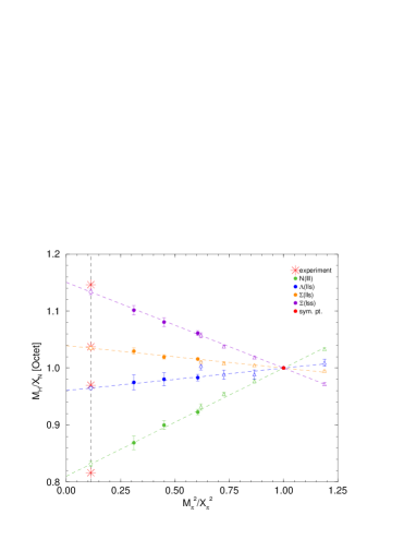
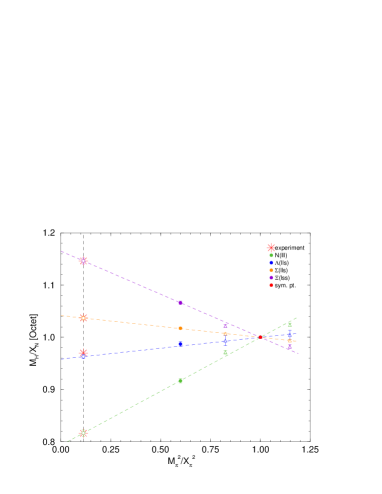
Figure 1: $M_{H}/X_{N}$ ($H=N$, $\Lambda$, $\Sigma$, $\Xi$) against $M_{\pi}^{2}/X_{\pi}^{2}$ for an initial point (“sym. pt.”) on the flavour symmetric line given by $\kappa_{0}=0.12090$, left panel, and $\kappa_{0}=0.12092$, right panel. The $32^{3}\times 64$ lattices are filled circles, while the $24^{3}\times 48$ lattices are open triangles. Also shown is the combined fit of eq. (37) (the dashed lines) to the $32^{3}\times 64$ lattice data. The fit results are the open circles, while the experimental points are the (red) stars. $l$ and $s$ denote the light and strange quark content of the hadron.

we plot the baryon octet $M_{H}/X_{N}$ for $H=N$, $\Lambda$, $\Sigma$, $\Xi$ against $M_{\pi}^{2}/X_{\pi}^{2}$ together with a linear fit, eq. (7) and implicitly eq. (33) using $2+1$ $O(a)$ improved clover fermions at $\beta=5.50$, [24] using two starting values for the quark mass on the flavour symmetric line, namely $\kappa_{0}=0.12090$, $0.12092$.

All the points have been arranged in the simulation to have constant $\overline{m}$. We see that a linear fit provides a good description of the numerical data from the symmetric point (where $M_{\pi}\sim X_{\pi}^{*}=410.9\,\mbox{MeV}$) down to the physical pion mass.

In a little more detail, the bare quark masses are defined as

$$am_{q}={1\over 2}\left({1\over\kappa_{q}}-{1\over\kappa_{0;c}}\right)\,,\qquad\mbox{with}\quad q=l,s,0\,,$$ (16)

(with the index $q=0$ denoting the common quark along the flavour symmetric line) and where vanishing of the quark mass along the $SU(3)$ flavour symmetric line determines $\kappa_{0;c}$. Keeping $\overline{m}=\mbox{constant}\equiv m_{0}$ gives

$$\kappa_{s}={1\over{{3\over\kappa_{0}}-{2\over\kappa_{l}}}}\,.$$ (17)

So once we decide on a $\kappa_{l}$ this then determines $\kappa_{s}$. Note that $\kappa_{0;c}$ drops out of eq. (17), so we do not need its explicit value. These initial $\kappa_{0}$ values chosen here, namely $\kappa_{0}=0.12090$ and $0.12092$ are close to the path that leads to the physical point ($\kappa_{0}=0.12092$ being slightly closer). (This is discussed in more detail in [23], which also contains numerical tables and phenomenological values for the hadron masses. Results not included there are given in Appendix C.) This path is also illustrated later in section 4.3, Fig. 4. Although finite size effects tend to cancel in ratios of quantities from the same multiplet, we nevertheless fit just to the results from the $32^{3}\times 64$ lattices (filled circles) using the linear fit of eq. (7). Finally note that we also have a similar flavour expansion for the pseudoscalar octet as for the baryon octet, as will be discussed in section 4.3.

3 (Hyperon) scalar matrix elements

Scalar matrix elements can be determined from the gradient of the hadron mass (with respect to the quark mass) by using the Feynman–Hellman theorem which is true for both bare and renormalised quantities. So if we take the derivative with respect to the bare quark mass we get the bare $\overline{q}q$ matrix element,

$${\partial M_{H}\over\partial m_{l}}=\langle H|(\overline{u}u+\overline{d}d)|H\rangle\,,\qquad{\partial M_{H}\over\partial m_{s}}=\langle H|\overline{s}s|H\rangle\,,$$ (18)

while if we take the derivative with respect to the renormalised quark mass we get the renormalised matrix element. In the left panel of Fig. 2, we show the

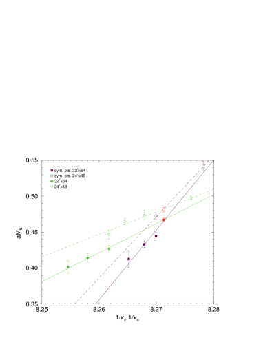
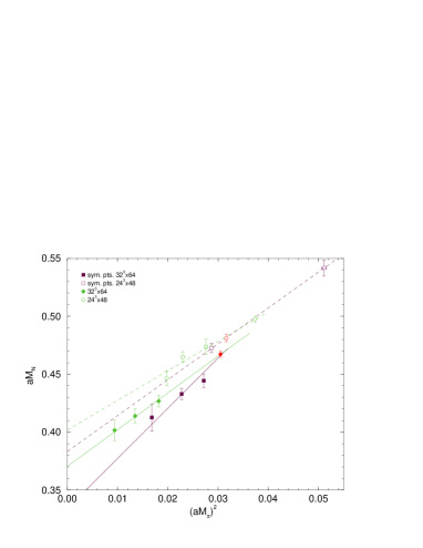
Figure 2: The left panel shows the nucleon mass, $aM_{N}$, versus $1/\kappa_{l}$, (for the $\overline{m}=\mbox{const.}$ points, green diamonds with $\kappa_{0}=0.12090$) and versus $1/\kappa_{0}$ (for the flavour symmetric points, “sym. pts.”, maroon squares). The common flavour symmetric points are denoted by red circles. The $24^{3}\times 48$ volume results are open symbols together with a dashed line for the (linear) fit, while the $32^{3}\times 64$ volume results are filled symbols and solid lines. Similarly the right panel shows the nucleon mass $aM_{N}$, versus $(aM_{\pi})^{2}$ (same notation as for the left panel).

nucleon masses (green diamonds) and the flavour symmetric nucleon masses (maroon squares) against $1/\kappa_{l}$, $1/\kappa_{0}$ respectively (from eq. (16) these are proportional to the bare quark mass). From the Feynman–Hellmann theorem, the slope of the masses (maroon squares) gives the total $\sum_{q=u,d,s}\langle N|\overline{q}q|N\rangle$, while the slope of the masses (green diamonds) gives the valence contribution. The difference between the two contributions gives the disconnected contribution. Because here all three quark masses are equal, the disconnected contribution for all three quarks will be the same. The two slopes thus give the estimates

$${\sum_{q}\langle N|\overline{q}q|N\rangle_{con}\over\sum_{q}\langle N|\overline{q}q|N\rangle} \sim {4.0\over 9.7}\sim 0.41$$

$${\langle N|\overline{s}s|N\rangle\over\sum_{q}\langle N|\overline{q}q|N\rangle} \sim {1\over 3}\left(9.7-4.0\over 9.7\right)\sim 0.19\,,$$ (19)

for bare lattice quantities.

To look at renormalised matrix elements, we need a plot against the renormalised mass, $(aM_{\pi})^{2}$ (as in leading order PCAC, $M_{\pi}^{2}$ is proportional to the renormalised quark mass, eq. (35)). This is shown in the right panel of Fig. 2. The slopes are now much closer to each other. We now find the estimates

$${\sum_{q}\langle N|(\overline{q}q)^{\mbox{\tiny$R$}}|N\rangle_{con}\over\sum_{q}\langle N|(\overline{q}q)^{\mbox{\tiny$R$}}|N\rangle} \sim {3.2\over 4.3}\sim 0.74$$

$${\langle N|(\overline{s}s)^{\mbox{\tiny$R$}}|N\rangle\over\sum_{q}\langle N|(\overline{q}q)^{\mbox{\tiny$R$}}|N\rangle} \sim {1\over 3}\left(4.3-3.2\over 4.3\right)\sim 0.085\,,$$ (20)

for renormalised lattice quantities, giving $y^{(N)\mbox{\tiny$R$}}\sim 2\times 0.085/(1-0.085)\sim 0.19$. So although for bare matrix elements, there is a significant strange quark content this is reduced in the renormalised matrix element.

We shall now try to make these considerations a little more quantitive.

4 (Hyperon) $\sigma$ equations

4.1 Renormalisation

For Wilson (clover) fermions under renormalisation the singlet and non-singlet pieces of the quark mass renormalise differently [25, 26]. We have

$$m_{q}^{\mbox{\tiny$R$}}=Z^{\mbox{\tiny$N\!S$}}\left[m_{q}+\alpha_{Z}\mbox{\small$\frac{1}{3}$}(2m_{l}+m_{s})\right]\,,\qquad\alpha_{Z}={Z^{\mbox{\tiny$S$}}-Z^{\mbox{\tiny$N\!S$}}\over Z^{\mbox{\tiny$N\!S$}}}\,.$$ (21)

In the action the term $\sum_{q}m_{q}\overline{q}q=\sum_{q}m_{q}^{\mbox{\tiny$R$}}(\overline{q}q)^{\mbox{\tiny$R$}}$ i.e. a renormalisation group invariant or RGI quantity. Upon writing this in a matrix form and inverting gives

$$(\overline{q}q)^{\mbox{\tiny$R$}}={1\over Z^{\mbox{\tiny$N\!S$}}}\left[\overline{q}q-{\alpha_{Z}\over 1+\alpha_{Z}}\mbox{\small$\frac{1}{3}$}(\overline{u}u+\overline{d}d+\overline{s}s)\right]\,,$$ (22)

so for $\alpha_{Z}\not=0$ then there is always mixing between bare operators.

As an example of where this manifests itself, the relation between the bare, $y^{(H)}$, and renormalised $y^{(H)\mbox{\tiny$R$}}$, cf. eq. (2), is then given by

$$y^{(H)\mbox{\tiny$R$}}={y^{(H)}-\mbox{\small$\frac{2}{3}$}\alpha_{Z}(1-y^{(H)})\over 1+\mbox{\small$\frac{1}{3}$}\alpha_{Z}(1-y^{(H)})}\,,$$ (23)

so we see that $y^{(H)\mbox{\tiny$R$}}\not=y^{(H)}$ for clover fermions. Additionally, since $\alpha_{Z}>0$ and $y^{(H)}\mathrel{\hbox to0.0pt{\lower 4.0pt\hbox{\hskip 1.0pt$\sim$}\hss}\raise 1.0pt\hbox{$>$}}0$ we find that $y^{(H)\mbox{\tiny$R$}}<y^{(H)}$, i.e. is reduced.

Useful quark combinations are the octet and singlet combinations, namely

$$(\overline{u}u+\overline{d}d)^{\mbox{\tiny$R$}}-2(\overline{s}s)^{\mbox{\tiny$R$}} = {1\over Z^{\mbox{\tiny$N\!S$}}}\,\left[(\overline{u}u+\overline{d}d)-2(\overline{s}s)\right]\,,$$

$$(\overline{u}u+\overline{d}d)^{\mbox{\tiny$R$}}+(\overline{s}s)^{\mbox{\tiny$R$}} = {1\over Z^{\mbox{\tiny$N\!S$}}(1+\alpha_{Z})}\,\left[(\overline{u}u+\overline{d}d)+(\overline{s}s)\right]\,.$$ (24)

Furthermore, using the Feynman-Hellman theorem, eq. (18) and with the hadron flavour expansion, eq. (7) together with eq. (15) gives

$$\langle H|(\overline{u}u+\overline{d}d)^{\mbox{\tiny$R$}}-2(\overline{s}s)^{\mbox{\tiny$R$}}|H\rangle = {1\over Z^{\mbox{\tiny$N\!S$}}}\,c_{H}$$ (25)

$$\langle H|(\overline{u}u+\overline{d}d)^{\mbox{\tiny$R$}}+(\overline{s}s)^{\mbox{\tiny$R$}}|H\rangle = {1\over Z^{\mbox{\tiny$N\!S$}}}\,{M_{0}^{\prime}\over 1+\alpha_{Z}}\,.$$ (26)

Eq. (25), the equation for the matrix element of an octet operator, only involves $c_{H}$ (the hadron mass expansion keeping the singlet quark mass constant), while eq. (26), the matrix element of a singlet operator, only involves $M_{0}^{\prime}$ (occuring when changing the singlet quark mass). Eq. (25) also leads to eq. (3) as discussed in the introduction.

Finally note that the quantities

$$(m_{s}-m_{l})\langle H|(\overline{u}u+\overline{d}d)-2\overline{s}s|H\rangle\,,\quad(2m_{l}+m_{s})\langle H|(\overline{u}u+\overline{d}d)+\overline{s}s|H\rangle\,,$$ (27)

are RGI, all $Z$ factors cancel when they are renormalised. Linear combinations of these two quantities are also RGI in particular the combination used previously of $\sigma_{l}^{(H)}+\sigma_{s}^{(H)}=\sum_{q}m_{q}\langle H|\overline{q}q|H\rangle$. However, $\sigma_{l}^{(H)}$ and $\sigma_{s}^{(H)}$ considered separately are not RGI, see eqs. (21), (22). The renormalised quantities are mixtures of the two lattice quantities, and $\alpha_{Z}$ is needed to relate lattice values to continuum values. Refering back to Fig. 2 we see that the bare lattice strange sigma term is much larger that the renormalised strange sigma term, due to a cancellation between the two terms in eq. (22).

4.2 $\sigma$ equations

Multiplying the renormalised quark mass, eq. (21), together with eqs. (25), (26) (or more generally with eq. (22)) we can find RGI combinations (i.e. a form where the renormalisation constant $Z^{\mbox{\tiny$N\!S$}}$ cancels). In particular we find

$$\sigma_{l}^{(H)}-2r\sigma_{s}^{(H)} = {3r\over 1+2r}(1+\alpha_{Z})m_{0}c_{H}$$ (28)

$$\sigma_{l}^{(H)}+r\sigma_{s}^{(H)} = {3r\over 1+2r}m_{0}M_{0}^{\prime}(m_{0})\,,$$ (29)

where $r$ is the ratio of quark masses

$$r\equiv{m_{l}^{\mbox{\tiny$R$}}\over m_{s}^{\mbox{\tiny$R$}}}\,.$$ (30)

Thus we have to find the (fixed) coefficients $(1+\alpha_{Z})m_{0}c_{H}$, $m_{0}M_{0}^{\prime}(m_{0})$. We then determine the physical values of the sigma terms by extrapolating to the point where the quark mass ratio takes its physical value, i.e. $r=r^{*}$.

We observe that we have two simultaneous equations, which can be easily solved to give

$$\sigma_{l}^{(H)} = {r\over 1+2r}\,\left[(1+\alpha_{Z})m_{0}c_{H}+2m_{0}M^{\prime}_{0}(m_{0})\right]$$

$$\sigma_{s}^{(H)} = {1\over 1+2r}\,\left[-(1+\alpha_{Z})m_{0}c_{H}+m_{0}M^{\prime}_{0}(m_{0})\right]\,.$$ (31)

We see that the smallness of $\sigma_{l}^{(H)}$ in comparison to $\sigma_{s}^{(H)}$ is certainly guaranteed by the presence of an additional $r$ in its numerator. As $\sigma_{s}^{(H)}>0$ we must also have $M^{\prime}_{0}(m_{0})>(1+\alpha_{Z})\max c_{H}$. These coefficients are also sufficient to determine $y^{(H)\mbox{\tiny$R$}}$, as can be seen either directly from eq. (31) or from eq. (26),

$$y^{(H)\mbox{\tiny$R$}}=2\,{-(1+\alpha_{Z})m_{0}c_{H}+m_{0}M^{\prime}_{0}(m_{0})\over(1+\alpha_{Z})m_{0}c_{H}+2m_{0}M^{\prime}_{0}(m_{0})}\,.$$ (32)

Again, as seen in section 3, $y^{(H)\mbox{\tiny$R$}}$ only depends on gradients and not on the physical point.

It is now convenient to normalise the coefficients by $X_{N}$ so we now need to find the coefficients $(1+\alpha_{Z})m_{0}c_{H}/X_{N}(m_{0})$ and $m_{0}M^{\prime}_{0}(m_{0})/X_{N}(m_{0})$.

4.3 Determination of the coefficients

The hint for determining the coefficients from our lattice data is given in section 3, where we consider gradients with respect to a renormalised or physical quantity – here taken as the pion mass. As in eq. (7) we also have a similar expansion for the pseudoscalar octet,

$$M_{\pi}^{2}=M_{0\,\pi}^{2}+2\alpha\delta m_{l}+O(\delta m_{l}^{2})\,,$$ (33)

(together with $M_{K}^{2}=M_{0\,\pi}^{2}-\alpha\delta m_{l}+O(\delta m_{l}^{2})$, $M_{\eta_{s}}^{2}=M_{0\,\pi}^{2}-4\alpha\delta m_{l}+O(\delta m_{l}^{2})$). This gives a good representation of the data as can be seen from Fig. 12 of [23]. Analogously to eq. (14) we can define a flavour singlet quantity

$$X_{\pi}^{2}=\mbox{\small$\frac{1}{3}$}(2M_{K}^{2}+M_{\pi}^{2})=M_{0\,\pi}^{2}+O(\delta m_{l}^{2})\,.$$ (34)

However, as well as eq. (7), we have the additional constraint from PCAC

$$M_{\pi}^{2}=2B_{0}^{\mbox{\tiny$R$}}m_{l}^{\mbox{\tiny$R$}}\,,$$ (35)

(together with $M_{K}^{2}=B_{0}^{\mbox{\tiny$R$}}(m_{l}^{\mbox{\tiny$R$}}+m_{s}^{\mbox{\tiny$R$}})$, $M_{\eta_{s}}^{2}=2B_{0}^{\mbox{\tiny$R$}}m_{s}^{\mbox{\tiny$R$}}$) which implies that

$$M_{0\,\pi}^{2}=2\alpha(1+\alpha_{Z})\overline{m}\,,\qquad\alpha=B_{0}^{\mbox{\tiny$R$}}Z^{\mbox{\tiny$N\!S$}}\,.$$ (36)

If we now consider an expansion in the (physical) pion mass then eliminating $\delta m_{l}$ between eq. (7) and eq. (33) gives

$${M_{H}\over X_{N}}=\left(1-\left[(1+\alpha_{Z})m_{0}{c_{H}\over X_{N}}\right]\right)+\left[(1+\alpha_{Z})m_{0}{c_{H}\over X_{N}}\right]\,{M_{\pi}^{2}\over X_{\pi}^{2}}\,,$$ (37)

from the point on the symmetric line $m_{0}=\overline{m}$. Thus if we plot $M_{H}/X_{N}$ versus $M_{\pi}^{2}/X_{\pi}^{2}$ (holding the singlet quark mass, $\overline{m}$ constant) then the gradient immediately yields $(1+\alpha_{Z})m_{0}c_{H}/X_{N}$. The only assumption is that the ‘fan’ plot splittings remain linear in $\delta m_{l}$ down to the physical point. In Fig. 1 we show this plot giving the results

$$(1+\alpha_{Z})m_{0}{3A_{1}\over X_{N}}= 0.1899(55)\,, 0.2066(68)\,,$$

$$(1+\alpha_{Z})m_{0}{3A_{2}\over X_{N}}= 0.03942(314)\,, 0.04164(431)\,,$$ (38)

for $\kappa_{0}=0.12090$, $0.12092$ respectively.

Alternatively on the flavour symmetric line, $m_{l}=\overline{m}$ (i.e. $\delta m_{l}=0$), so varying $\overline{m}$ from a point $m_{0}$ gives

$$M_{\pi}^{2}(\overline{m})=M_{0\,\pi}^{2}(\overline{m}) = M_{0\,\pi}^{2}(m_{0})+M_{0\,\pi}^{2\,\prime}(m_{0})(\overline{m}-m_{0})$$ (39)

$$= 2\alpha(1+\alpha_{Z})[m_{0}+(\overline{m}-m_{0})]\,,$$

which gives $M_{0\,\pi}^{2\,\prime}(m_{0})=2\alpha(1+\alpha_{Z})$. So now eliminating $(\overline{m}-m_{0})$ between eqs. (15), (39) gives

$${X_{N}(\overline{m})\over X_{N}(m_{0})}=\left(1-\left[{m_{0}M_{0}^{\prime}(m_{0})\over X_{N}(m_{0})}\right]\right)+\left[{m_{0}M_{0}^{\prime}(m_{0})\over X_{N}(m_{0})}\right]\,{X_{\pi}^{2}(\overline{m})\over X_{\pi}^{2}(m_{0})}\,.$$ (40)

Again in a plot of $X_{N}(\overline{m})/X_{N}(m_{0})$ versus $X_{\pi}^{2}(\overline{m})/X_{\pi}^{2}(m_{0})$ the gradient immediately gives the required ratio $m_{0}M_{0}^{\prime}(m_{0})/X_{N}(m_{0})$. We have also replaced $M_{N}$ by $X_{N}$ and $M_{\pi}^{2}$ by $X_{\pi}^{2}$ (which allows us to use all the $32^{3}\times 64$ data available for a particular $\overline{m}$). In Fig. 3 we plot

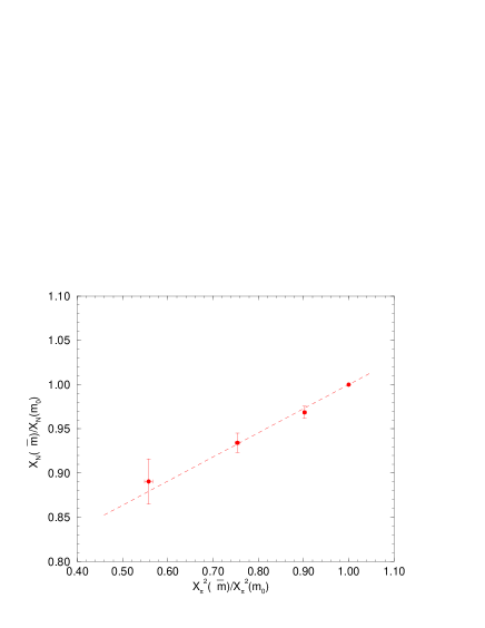
Figure 3: $X_{N}(\overline{m})/X_{N}(m_{0})$ versus $X_{\pi}^{2}(\overline{m})/X_{\pi}^{2}(m_{0})$ along the flavour symmetric line, together with the linear fit from eq. (40).

$X_{N}(\overline{m})/X_{N}(m_{0})$ versus $X_{\pi}^{2}(\overline{m})/X_{\pi}^{2}(m_{0})$. From eq. (40) this gives

$${m_{0}M_{0}^{\prime}(m_{0})\over X_{N}(m_{0})}=0.273(32)\,.$$ (41)

Finally the quark mass ratio, $r$, must be estimated. In Fig. 4

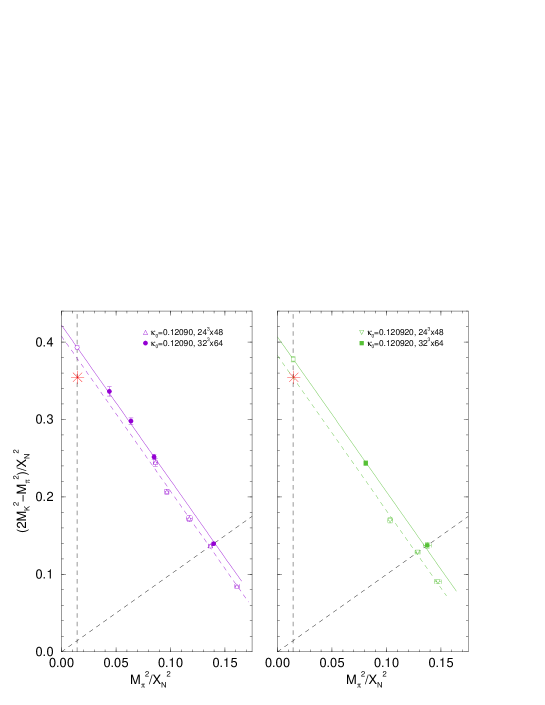
Figure 4: $(2M_{K}^{2}-M_{\pi}^{2})/X_{N}^{2}$ versus $M_{\pi}^{2}/X_{N}^{2}$ for $\kappa_{0}=0.12090$ (left panel) and $\kappa_{0}=0.12092$ (right panel). The $32^{3}\times 64$ volume results are given by the filled symbols, while the $24^{3}\times 48$ volume results are shown using empty triangles. The fit is given in eq. (42). Experimental points are denoted by (red) stars.

we plot $(2M_{K}^{2}-M_{\pi}^{2})/X_{N}^{2}$ versus $M_{\pi}^{2}/X_{N}^{2}$. From eq. (33) we have

$${2M_{K}^{2}-M_{\pi}^{2}\over X_{N}^{2}}=3{M_{0\pi}^{2}\over X_{N}^{2}}-2{M_{\pi}^{2}\over X_{N}^{2}}\,.$$ (42)

As in section 2, we see that for constant $\overline{m}$ the data points lie on a straight line (i.e. there is an absence of significant non-linearity). Furthermore the gradient is fixed at $-2$. (Indeed leaving the gradient as a fit parameter for the $\kappa_{0}=0.12090$ confirms that this gradient is very close to $-2$.) Together with PCAC, eq. (35) this gives the $x$-axis is proportional to $m_{l}^{\mbox{\tiny$R$}}$ while the $y$-axis is proportional to $m_{s}^{\mbox{\tiny$R$}}$ and thus the ratio gives $r$. Taking our physical scale to be defined from $M_{\pi}^{2}/X_{N}^{2}|^{*}$ (i.e. from the $x$-axes of Fig. 4) gives

$${1\over r^{*}}=\left.{m_{s}^{\mbox{\tiny$R$}}\over m_{l}^{\mbox{\tiny$R$}}}\right|^{*}=\left\{\begin{array}[]{cc}27.28(16)&\kappa_{0}=0.12090\\ 26.23(24)&\kappa_{0}=0.12092\\ \end{array}\right.\,.$$ (45)

4.4 Curvature effects

What can we say about corrections to the linear terms? The simple linear fit describes the data well, from the symmetric point to our lightest pion mass, both along the $\overline{m}=\mbox{const.}$ line and the flavour symmetric line. To see qualitatively the possible influence of curvature we now compare linear fits with quadratic fits. These will be used to estimate possible systematic effects. We briefly discuss these effects here.

In Fig. 5

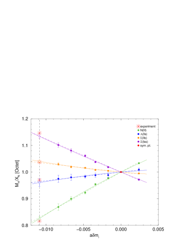
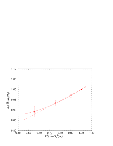
Figure 5: Left panel: $M_{H}/X_{N}$ for $H=N$, $\Lambda$, $\Sigma$, $\Xi$ against $a\delta m_{l}$ for initial point on the flavour symmetric line given by $\kappa_{0}=0.12090$ together with the previous linear fit (dashed lines) and quadratic fit (solid lines). Other notation as in Fig. 1. Right panel: $X_{N}(\overline{m})/X_{N}(m_{0})$ versus $X_{\pi}^{2}(\overline{m})/X_{\pi}^{2}(m_{0})$ along the flavour symmetric line, together with a linear fit from eq. (40) (dashed line) and a quadratic fit (solid line).

we compare the results of a quadratic fit and a linear fit, both for the baryon mass fan plot and for $X_{N}(\overline{m})/X_{N}(m_{0})$. In the left panel of the figure, we consider the baryon mass fan plot. The quadratic fit here uses all the data, [23], on both lattice sizes (in cases where results for two lattice sizes are available, we used the larger lattice size only). The curvature terms here are small and statistically compatible with zero.

The right panel of the figure shows a quadratic fit to the results along the symmetric line. The curvature here is dominated by the large error of the lightest point (which has a low statistic). Thus we shall regard this fit as only giving an estimation of the possible systematic error.

The results in the next section include systematic error estimates from both these curvature sources combined in quadrature. In Appendix B we give some more details.

5 Results

We can now numerically determine $y^{(H)\mbox{\tiny$R$}}$ and $\sigma_{l}^{(H)}$, $\sigma_{s}^{(H)}$.

We start with $y^{(H)\mbox{\tiny$R$}}$. From eq. (32), together with eqs. (38), (41) and eq. (12) gives the results in Table 1.

	$N$	$\Lambda$	$\Sigma$	$\Xi$
$\kappa_{0}=0.12090$
$y^{(H)\mbox{\tiny$R$}*}$	0.22(9)(15)	0.80(14)(28)	1.23(20)(41)	2.14(38)(64)
$\sigma_{l}^{(H)*}\,\mbox{[MeV]}$	29(3)(4)	23(3)(4)	20(3)(4)	16(3)(5)
$\sigma_{s}^{(H)*}\,\mbox{[MeV]}$	89(34)(59)	250(34)(68)	334(34)(68)	453(34)(58)
$\kappa_{0}=0.12092$
$y^{(H)\mbox{\tiny$R$}*}$	0.18(9)(15)	0.79(14)(28)	1.25(20)(42)	2.30(42)(68)
$\sigma_{l}^{(H)*}\,\mbox{[MeV]}$	31(3)(4)	24(3)(4)	21(3)(4)	16(3)(4)
$\sigma_{s}^{(H)*}\,\mbox{[MeV]}$	71(34)(59)	247(34)(69)	336(34)(69)	468(35)(59)

Table 1: Results for the baryon octet for $y^{(H)\mbox{\tiny$R$}*}$, $\sigma_{l}^{(H)*}$, $\sigma_{s}^{(H)*}$ with $H=N$, $\Lambda$, $\Sigma$, $\Xi$ for $\kappa_{0}=0.12090$, $0.12092$.

The first error is the linear fit error (in this case dominated by the error in eq. (41)), while the second error indicates possible effects from higher order terms, as discussed in section 4.4. We see that there is an order of magnitude increase in the fraction of $\langle H|(\overline{s}s)^{\mbox{\tiny$R$}}|H\rangle$ compared to $\langle H|(\overline{u}u+\overline{d}d)^{\mbox{\tiny$R$}}|H\rangle$ as we increase the strangeness content of the baryon from the nucleon (no valence strange quarks) to the $\Xi$ (two valence strange quarks).

Turning to the sigma terms themselves, from eq. (28) we can find an indication of the magnitude of $\sigma^{(N)}_{l}$ as approximately (with $X_{N}=1.1501\,\mbox{GeV}$),

$$\sigma_{l}^{(N)\,*}\sim[22\sim 25]+{\sigma_{s}^{(N)\,*}\over 13}\,\mbox{MeV}>[22\sim 25]\,\mbox{MeV}\,,$$ (46)

(for $\kappa_{0}=0.12090$, $0.12092$ respectively). The last inequality follows as obviously $\sigma_{s}^{(N)*}>0$. Indeed this shows that a non-zero $\sigma_{s}^{(N)*}>0$ can only add a few MeV to this result.

The results for $\sigma_{l}^{(H)*}$ and $\sigma_{s}^{(H)*}$ are also given in Table 1. (Again the first error is the statistical error, while the second systematic error is due to possible quadratic effects.) While the data for $\kappa_{0}=0.12090$ is more complete than for $\kappa_{0}=0.12092$ (cf. the plots in Fig. 1) and demonstrates linear behaviour, as the path starting at $\kappa_{0}=0.12092$ is closer to the physical point (cf. Fig. 4) we shall use these values as our final values. These results are illustrated in Fig. 6 for $y^{(H)\mbox{\tiny$R$}*}$

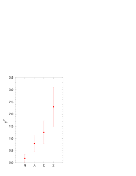
Figure 6: $y^{(H)\mbox{\tiny$R$}*}$ for $H=N$, $\Lambda$, $\Sigma$, $\Xi$ using the results from Table 1 for $\kappa_{0}=0.12092$.

where $H=N$, $\Lambda$, $\Sigma$, $\Xi$.

By varying $r$ in eq. (31) , we plot in Fig. 7

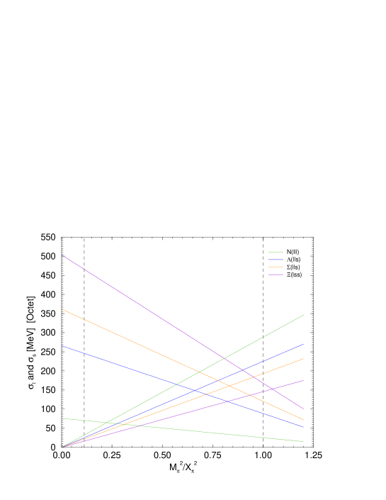
Figure 7: $\sigma_{l}^{(H)}$ (decreasing from the symmetric point $x=1$) and $\sigma_{s}^{(H)}$ (increasing) for $H=N$, $\Lambda$, $\Sigma$, $\Xi$ for $\kappa_{0}=0.12092$. The physical and symmetric lines are denoted by vertical dashed lines.

$\sigma_{l}^{(H)}$ and $\sigma_{s}^{(H)}$ for the baryon octet, $H=N$, $\Lambda$, $\Sigma$ and $\Xi$ from the symmetric point (vertical dashed line at $x=1$) to the physical point (left vertical dashed line). $\sigma_{l}^{(H)}$ is rapidly decreasing while $\sigma_{s}^{(H)}$ is increasing as we decrease the quark mass. Also, as expected $\sigma_{l}^{(H)}$ is largest for the nucleon, $N$, while $\sigma_{s}^{(N)}$ is the smallest. Finally in Fig. 8 we plot

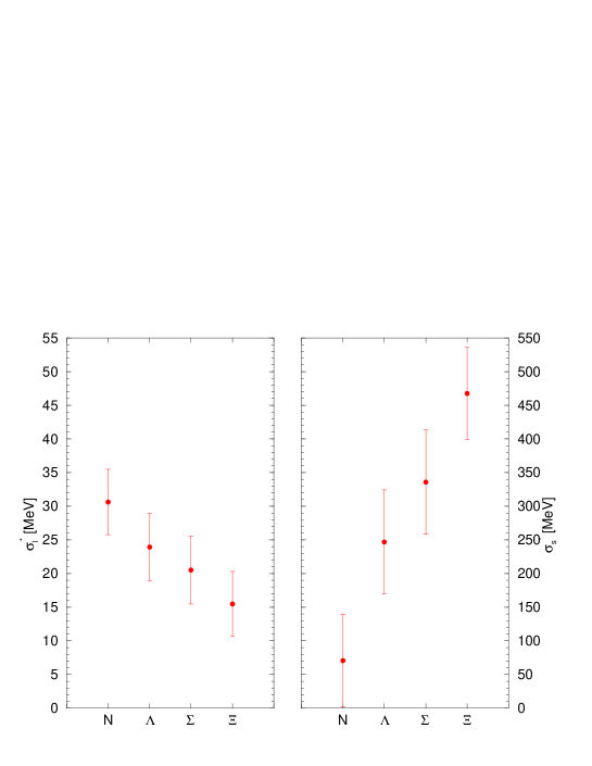
Figure 8: $\sigma_{l}^{(H)*}$ and $\sigma_{s}^{(H)*}$ for $H=N$, $\Lambda$, $\Sigma$, $\Xi$ at the physical point for $\kappa_{0}=0.12092$.

$\sigma_{l}^{(H)*}$, $\sigma_{s}^{(H)*}$ against $H=N$, $\Lambda$, $\Sigma$ and $\Xi$, again using Table 1.

6 Conclusions

Keeping the average quark mass constant gives very linear ‘fan’ plots from the flavour symmetric point down to the physical point. This implies that an expansion in the quark mass from the flavour symmetric point will give information about the physical point. In this article we have applied this to estimating the sigma terms (both light and strange) of the nucleon octet. There has been no use of a chiral perturbation expansion (indeed this is an opposite expansion to the one used here, expanding about zero quark mass).

Our results are given in section 5 and we quote from there a value for the nucleon sigma terms of

$$\sigma_{l}^{(N)*}=31(3)(4)\,\mbox{MeV}\,,\quad\sigma_{s}^{(N)*}=71(34)(59)\,\mbox{MeV}\,.$$ (47)

(The first error is the fit error while the second error indicates possible effects from higher order terms in the flavour expansion.) Note that expansions about the $SU(3)$ flavour line require consistency between many QCD observables, here for example not only for the baryon octet under consideration here, but also for the pseudoscalar octet, and PCAC and the ratio of the light to strange quark mass.

Of course there are several more avenues to investigate. Numerically an increase in statistics for the masses along the flavour symmetric line would reduce the dominant error (both statistical and systematic) and so directly help in decreasing the present errors. Our approach here has been to emphasise linearity at the expense (presently) of reaching exactly the physical point. This can be addressed by interpolating between a small set of constant $\overline{m}$ lines about the physical point. Additionally the use of partial quenching will also help to get closer to the physical pion mass. With more data, a systematic investigation of quadratic quark mass terms in the flavour expansion should be considered, to reduce the systematic errors. Finally while the use of linear or quadratic terms along the line of constant $\overline{m}$ is unproblematic, so that it is unlikely that eq. (46) will change by much, more subtle is the relation involving $X(\overline{m})$ (i.e. the gradient when changing $\overline{m}$.) For the example of clover fermions we have $\tilde{g}^{2}(\overline{m})=(1+b_{g}a\overline{m})g^{2}$ which clearly does not change if $\overline{m}=\mbox{constant}$, but will slightly change when $\overline{m}$ does. However this is probably not a large effect (as $b_{g}$ seems small). For a discussion of some aspects of this issue see [29, 30].

Appendix

Appendix A Some relations between the $\sigma$ terms

We discuss here some relations between the sigma terms within a multiplet (here taken to be the baryon octet) which are exact within the linear case discussed here, but which we might expect to always be approximately true.

The singlet relation eq. (26) or eq. (29) is the same for every hadron. So in terms of sigma terms this becomes

$$\sigma_{l}^{(H)}+r\sigma_{s}^{(H)}\approx\sigma_{l}^{(H^{\prime})}+r\sigma_{s}^{(H^{\prime})}\,.$$ (48)

At the flavour symmetric point it follows from group theory that a singlet operator has the same value for every member of a multiplet, so eq. (48) must hold. But this can change if we move away from the symmetric point. (We shall briefly discuss this at the end of this section.)

We can find another collection of near identities by summing over a singlet combination of hadrons — this can be either a singlet of $S_{3}$ or a singlet of $SU(3)$. If we do this, the expectation values of $\overline{u}u$, $\overline{d}d$ and $\overline{s}s$ will be exactly equal at the flavour symmetry point, and stay again nearly equal away from the symmetry point. By this argument we expect

$$\sigma_{l}^{(\Lambda)}+\sigma_{l}^{(\Sigma)} \approx 2r\left(\sigma_{s}^{(\Lambda)}+\sigma_{s}^{(\Sigma)}\right)$$

$$\sigma_{l}^{(N)}+\sigma_{l}^{(\Sigma)}+\sigma_{l}^{(\Xi)} \approx 2r\left(\sigma_{s}^{(N)}+\sigma_{s}^{(\Sigma)}+\sigma_{s}^{(\Xi)}\right)\,.$$ (49)

(Again this relation, as with the other relations discussed here, is exactly true for the linear case.)

Other relations come from the Gell-Mann–Okubo relation, [27, 28] in which the $27$-plet mass combination is very small,

$$2M_{N}-3M_{\Lambda}-M_{\Sigma}+2M_{\Xi}\approx 0\,,$$ (50)

for all values of $m_{l},m_{s}$. In our approach, its derivatives are also near zero. We therefore expect

$$2\sigma_{l}^{(N)}-3\sigma_{l}^{(\Lambda)}-\sigma_{l}^{(\Sigma)}+2\sigma_{l}^{(\Xi)} \approx 0$$

$$2\sigma_{s}^{(N)}-3\sigma_{s}^{(\Lambda)}-\sigma_{s}^{(\Sigma)}+2\sigma_{s}^{(\Xi)} \approx 0\,.$$ (51)

We obtain an even stronger version of these relations by taking the singlet combination, proportional to $(\overline{u}u+\overline{d}d)^{\mbox{\tiny$R$}}+(\overline{s}s)^{\mbox{\tiny$R$}}$,

$$2\sigma_{l}^{(N)}-3\sigma_{l}^{(\Lambda)}-\sigma_{l}^{(\Sigma)}+2\sigma_{l}^{(\Xi)}+r\left(2\sigma_{s}^{(N)}-3\sigma_{s}^{(\Lambda)}-\sigma_{s}^{(\Sigma)}+2\sigma_{s}^{(\Xi)}\right)\approx 0\,.$$ (52)

There is also a relation between the sigma terms and the hadron masses, [2] as the constants $A_{1}$ and $A_{2}$ which occur in the mass splittings also occur in the leading order expressions for the sigma terms. So there will be connections between masses and sigma terms. One particularly simple relation is

$$M_{H}-\sigma_{l}^{(H)}-\sigma_{s}^{(H)}\approx M_{H^{\prime}}-\sigma_{l}^{(H^{\prime})}-\sigma_{s}^{(H^{\prime})}\,.$$ (53)

(i.e. the baryon mass difference is closely accounted for by the sigma terms.) For the linear case this is again exact, with this equation being equal to $M_{0}(m_{0})-m_{0}M_{0}^{\prime}(m_{0})$ for all the octet baryons (upon using eqs. (7), (31)). From eq. (15) we see that this is just the common hadron mass in the chiral limit along the flavour symmetric line, when $m_{l}=0=m_{s}$ or $\overline{m}=0$. $\sigma_{l}^{(H)}$ and $\sigma_{s}^{(H)}$ can be thought of as that part of the hadron mass which is due to $m_{l}$ and $m_{s}$ respectively. The remnant, $M_{0}(m_{0})-m_{0}M_{0}^{\prime}(m_{0})$, is the part of the hadron mass due to the quark and gluon kinetic energy, interaction energy, etc., [2], i.e. the part of the hadron mass which is not due to the coupling with the Higgs vacuum expectation value.

We can use the higher order mass equations in [23] to estimate how well the relations in this section hold. Most of the relations have violations proportional to the first power of the $SU(3)$ breaking parameter, $\delta m_{l}$. The corrections to eqs. (48) and (49) and the first relation in eq. (51) are $O(m_{l}\delta m_{l})$. The $\sigma_{s}$ relation in eq. (51) has corrections $O(m_{s}\delta m_{l})$. When we combine these two relations to form eq. (52), the leading violation terms cancel, and we have a relation with corrections $O(m_{l}\delta m_{l}^{2})$. The corrections to the mass relation eq. (53) are $O(\overline{m}\delta m_{l})$ and $O(\delta m_{l}^{2})$.

Appendix B Higher order effects

In this Appendix, we discuss a little more quantitatively the systematic errors induced by the inclusion of the quadratic terms in the fit formulae. We concentrate particularly on the nucleon sigma terms, $\sigma_{l}^{(N)}$ and $\sigma_{s}^{(N)}$.

B.1 Curvature in the ‘fan’ plot

In Fig. 5 we compare the results of a quadratic fit and a linear fit, both for the baryon mass fan plot and on $\sigma_{l}^{(N)}$ and $\sigma_{s}^{(N)}$. The quadratic fit uses all the data, [23], on both lattice sizes (in cases where results for two lattice sizes are available, we used the larger lattice size only). Including curvature terms in eq. (7), [23], we have $M_{H}=M_{0}+c_{H}\delta m_{l}+b_{H}\delta m_{l}^{2}+\ldots$. Tracing through the analysis, we find the effect on eq. (31) is to replace

$$c_{H}\to c_{H}+2b_{H}\delta m_{l}\,.$$ (54)

By comparing $c_{H}$ from the linear fit with $c_{H}+2b_{H}\delta m_{l}^{*}$ from the quadratic fit, we can estimate the maximum possible change.

We use the data at $\kappa_{0}=0.12090$, because this is the case where we have the most data, covering the largest range in quark mass splitting, $\delta m_{l}$. In this case we have data covering about $3/4$ of the gap from the symmetric point to the physical point, so we have the most chance of seeing curvature effects if they are present.

For the fan plot (left panel of Fig. 5), the curvature terms are found to be small, and statistically compatible with zero curvature. In Fig. 9 we compare the nucleon sigma terms

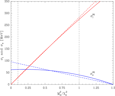
Figure 9: $\sigma_{l}^{(N)}$ (decreasing red lines from right to left) and $\sigma_{s}^{(N)}$ (increasing blue lines from right to left) against $M_{\pi}^{2}/X_{\pi}^{2}$ using linear fits (dashed lines) and quadratic fits (solid lines) for $\kappa_{0}=0.12090$.

from the slopes of the two fits by using eq. (31) together with eq. (54). Again we see that the curvature effect is very small in the case of $\sigma_{l}^{(N)}$, particularly at small $m_{l}$, and much larger for $\sigma_{s}^{(N)}$. Can we explain this difference?

The slopes in the fan plot only effect the non-singlet matrix element, the $c_{H}$ term in eq. (31). The curvature changes the slope of the nucleon line by about $10\%$ at the physical point. The non-singlet term in $\sigma_{l}^{(N)}$ is responsible for about $25\%$ of the quantity, so a $10\%$ change in slope translates to a $2.5\%$ change in $\sigma_{l}^{(N)}$. Putting in the actual slope change, the final number we arrive at is a systematic uncertainty of about $1\,\mbox{MeV}$ in $\sigma_{l}^{(N)}$ coming from curvature in the fan plot.

The situation for $\sigma_{s}^{(N)}$ is different, the singlet and non-singlet terms appear with opposite signs, so $\sigma_{s}^{(N)}$ is given by the difference between two large quantities. Thus a $10\%$ change in the non-singlet matrix element is leveraged into a $25\%$ change in $\sigma_{s}^{(N)}$. Repeating this procedure for the other hadrons gives similar non-singlet uncertainties.

B.2 Curvature along the symmetric line

We also use a linear fit to describe the baryon masses along the symmetric line (the line with all three quark masses equal). What is the effect of using a quadratic fit to determine the slope along this line?

In the right panel of Fig. 5 we compare a quadratic and linear fit to the symmetric baryon masses. As before, the quadratic term is compatible with zero curvature. Indeed the quadratic term is probably too large and is likely due to having a short lever arm and low statistics at the lightest point rather than to be a real effect. (Also we would expect that chiral perturbation theory would predict a downward curve.)

Feeding these values into eq. (31) gives an estimate of the possible effect of quadratic terms, due to curvature along the symmetric line, which we will include in our final error estimate. This curvature effect is the same for every hadron, giving an uncertainty $\sim 4\,\mbox{MeV}$ for $\sigma_{l}$ and $\sim 55\,\mbox{MeV}$ for $\sigma_{s}$. However because the shift is universal, this does not effect splittings, so the systematic error in $\sigma_{l}^{(H)}-\sigma_{l}^{(H^{\prime})}$ is still given by the $\sim 1\,\mbox{MeV}$ value of the previous subsection. For $y^{(H)\mbox{\tiny$R$}}$, using the first equation in eq. (4) gives percentage changes in $y^{(N)\mbox{\tiny$R$}}$ of $60\%$ and $30\%$ for $y^{(\Lambda)\mbox{\tiny$R$}}$, $y^{(\Sigma)\mbox{\tiny$R$}}$ and $y^{(\Xi)\mbox{\tiny$R$}}$.

Appendix C Hadron Masses

We collect here in Tables (2) – (5) numerical values for the meson pseudoscalar octet and baryon octet, not given in [23]. (All the data sets used here are over $\sim 2000$ configurations for the $24^{3}\times 48$ volumes and $\sim 1500-2000$ configurations for the $32^{3}\times 64$ volumes except for $\kappa_{0}=0.12099$ which has $\sim 500$ configurations.) Errors are from a bootstrap analysis.

$\kappa_{0}$	$aM_{\pi}$	$aM_{N}$
$32^{3}\times 64$
0.120920	0.1647(4)	0.4443(59)

Table 2: Additional result for the pseudoscalar octet mesons and octet baryons along the flavour symmetric line: $aM_{\pi}$, $aM_{N}$, for $(\beta,c_{sw},\alpha)=(5.50,2.65,0.1)$.

$(\kappa_{l},\kappa_{s})$	$aM_{\pi}$	$aM_{K}$	$aM_{\eta_{s}}$
$24^{3}\times 48$
(0.120870, 0.121020)	0.1804(8)	0.1621(10)	0.1407(12)
(0.120980, 0.120800)	0.1545(9)	0.1775(8)	0.1976(7)

Table 3: Additional results for the pseudoscalar octet mesons: $aM_{\pi}$, $aM_{K}$ and $aM_{\eta_{s}}$ for $(\beta,c_{sw},\alpha)=(5.50,2.65,0.1)$ where $\kappa_{0}=0.12092$.

$(\kappa_{l},\kappa_{s})$	$aM_{N}$	$aM_{\Lambda}$	$aM_{\Sigma}$	$aM_{\Xi}$
$24^{3}\times 48$
(0.120870, 0.121020)	0.4812(40)	0.4721(62)	0.4672(48)	0.4618(58)
(0.120980, 0.120800)	0.4668(61)	0.4773(62)	0.4838(47)	0.4909(41)

Table 4: Additional results for the octet baryons: $aM_{N}$, $aM_{\Lambda}$, $aM_{\Sigma}$ and $aM_{\Xi}$ for $(\beta,c_{sw},\alpha)=(5.50,2.65,0.1)$ where $\kappa_{0}=0.12092$.

$(\kappa_{l},\kappa_{s})$	$M_{N}/X_{N}$	$M_{\Lambda}/X_{N}$	$M_{\Sigma}/X_{N}$	$M_{\Xi}/X_{N}$
$24^{3}\times 48$
(0.120870, 0.121020)	1.024(3)	1.004(9)	0.9939(17)	0.9824(34)
(0.120980, 0.120800)	0.9715(33)	0.9934(95)	1.007(2)	1.022(3)
$32^{3}\times 64$
(0.121050, 0.120661)	0.9167(40)	0.9872(46)	1.017(2)	1.066(3)

Table 5: Additional ratio results for the octet baryons: $M_{N}/X_{N}$, $M_{\Lambda}/X_{N}$, $M_{\Sigma}/X_{N}$ and $M_{\Xi}/X_{N}$ for $(\beta,c_{sw},\alpha)=(5.50,2.65,0.1)$ where $\kappa_{0}=0.12092$.

References

- [1] T.-P. Cheng and L.-F. Li, Gauge Theory of Elementary Particles Oxford University Press (1988, reprinted); Schladming Winter School (March 1997), Computing Particle Properties (eds. C. B. Lang and H. Gausterer), Springer-Verlag, [arXiv:hep-ph/9709293].
- [2] X. Ji, Phys. Rev. Lett. 74 (1995) 1071, [arXiv:hep-ph/9410274].
- [3] R. Koch, Z. Phys. C15 (1982) 161.
- [4] J. Gasser, H. Leutwyler and M. E. Sainio, Phys. Lett. B253 (1991) 252; ibid 260.
- [5] M. M. Pavan, I. I. Strakovsky, R. L. Workman and R. A. Arndt, PiN Newslett. 16 (2002) 110, [arXiv:hep-ph/0111066].
- [6] B. Borasoy and U.-G. Meissner, Annals Phys. 254 (1997) 192, [arXiv:hep-ph/9607432].
- [7] J. Martin-Camalich, L. S. Geng and M. J. Vicente Vacas, Phys. Rev. D82 (2010) 074504, [arXiv:1003.1929[hep-lat]].
- [8] J. Ellis, K. A. Olive and P. Sandick, New J. Phys. 11 (2009) 105015, [arXiv:0905.0107[hep-ph]].
- [9] J. Giedt, A. W. Thomas and R. D. Young, Phys. Rev. Lett. 103 (2009) 201802, [arXiv:0907.4177[hep-ph]].
- [10] S. Güsken, K. Schilling, R. Sommer, K. H. Mütter and A. Patel, Phys. Lett. B212 (1988) 216.
- [11] R. Altmeyer, M. Göckeler, R. Horsley, E. Laermann and G. Schierholz, [MTc Collaboration], Nucl. Phys. Proc. Suppl. 34 (1994) 376, arXiv:hep-lat/9311020; Kyffhaeuser Workshop (Leipzig, Germany, September 1993), arXiv:hep-lat/9311012.
- [12] M. Fukugita, Y. Kuramashi, M. Okawa and A. Ukawa, Phys. Rev. D51 (1995) 5319, [arXiv:hep-lat/9408002].
- [13] S. J. Dong, J. F. Lagaë and K. F. Liu, Phys. Rev. D54 (1996) 5496, [arXiv:hep-ph/9602259].
- [14] S. Güsken, P. Ueberholz, J. Viehoff, N. Eicker, P. Lacock, T. Lippert, K. Schilling, A. Spitz and T. Struckmann, [SESAM Collaboration], Phys. Rev. D59 (1999) 054504, [arXiv:hep-lat/9809066].
- [15] A. Walker-Loud, H.-W. Lin, K. Orginos, D. G. Richards, R. G. Edwards, M. Engelhardt, G. T. Flemming, Ph. Hägler, B. Musch, M. F. Lin, H. B. Meyer, J. W. Negele, A. V. Pochinsky, M. Procura, S. Syritsyn, C. J. Morningstar, D. B. Renner and W. Schroers, Phys. Rev. D79 (2009) 054502, [arXiv:0806.4549[hep-lat]].
- [16] H. Ohki, H. Fukaya, S. Hashimoto, T. Kaneko, H. Matsufuru, J. Noaki, T. Onogi, E. Shintani and N. Yamada, [JLQCD Collaboration], Phys. Rev. D78 (2008) 054502, [arXiv:0806.4744[hep-lat]].
- [17] R. D. Young and A. W. Thomas, Phys. Rev. D81 (2010) 014503, [arXiv:0901.3310[hep-lat]].
- [18] K.-I. Ishikawa, N. Ishizuka, T. Izubuchi, D. Kadoh, K. Kanaya, Y. Kuramashi, Y. Namekawa, M. Okawa, Y. Taniguchi, A. Ukawa, N. Ukita and T. Yoshié, [PACS-CS Collaboration], Phys. Rev. D80 (2009) 054502, [arXiv:0905.0962[hep-lat]].
- [19] D. Toussaint and W. Freeman, [MILC Collaboration], Phys. Rev. Lett. 103 (2009) 122002, [arXiv:0905.2432[hep-lat]].
- [20] K. Takeda, S. Aoki, S. Hashimoto, T. Kaneko, J. Noaki and T. Onogi, [JLQCD Collaboration], Phys. Rev. D83 (2011) 114506, [arXiv:1011.1964[hep-lat]].
- [21] S. Dürr, Z. Fodor, T. Hemmert, C. Hoelbling, J. Frison, S. D. Katz, S. Krieg, T. Kurth, L. Lellouch, T. Lippert, A. Portelli, A. Ramos, A. Schäfer and K. K. Szabó, arXiv:1109.4265[hep-lat].
- [22] R. D. Young and A. W. Thomas, (4th Int. Symposium on Symmetries in Subatomic Physics (SSP2009), Taipei, Taiwan, June 2-5 2009), Nucl. Phys. A844 (2010) 266C-271C, arXiv:0911.1757[hep-lat].
- [23] W. Bietenholz, V. Bornyakov, M. Göckeler, R. Horsley, W. G. Lockhart, Y. Nakamura, H. Perlt, D. Pleiter, P. E. L. Rakow, G. Schierholz, A. Schiller, T. Streuer, H. Stüben, F. Winter and J. M. Zanotti, [QCDSF–UKQCD Collaboration], Phys. Rev. D84 (2011) 054509, [arXiv:1102.5300[hep-lat]].
- [24] N. Cundy, M. Göckeler, R. Horsley, T. Kaltenbrunner, A. D. Kennedy, Y. Nakamura, H. Perlt, D. Pleiter, P. E. L. Rakow, A. Schäfer, G. Schierholz, A. Schiller, H. Stüben and J. M. Zanotti, [QCDSF–UKQCD Collaboration], Phys. Rev. D79 (2009) 094507, [arXiv:0901.3302[hep-lat]].
- [25] M. Göckeler, R. Horsley, A. C. Irving, D. Pleiter, P. E. L. Rakow, G. Schierholz and H. Stüben, [QCDSF–UKQCD Collaboration], Phys. Lett. B639 (2006) 307, [arXiv:hep-ph/0409312].
- [26] P. E. L. Rakow, Nucl. Phys. Proc. Suppl. 140 (2005) 34, [arXiv:hep-lat/0411036].
- [27] M. Gell-Mann, Phys. Rev. 125 (1962) 1067.
- [28] S. Okubo, Prog. Theor. Phys. 27 (1962) 949.
- [29] C. Michael, C. McNeile and D. Hepburn, Nucl. Phys. Proc. Suppl. 106 (2002) 293, [arXiv:hep-lat/0109028].
- [30] R. Babich, R. C. Brower, M. A. Clark, G. T. Fleming, J. C. Osborn, C. Rebbi and D. Schaich, arXiv:1012.0562.
-
[31]
Y. Nakamura and H. Stüben,
PoS(Lattice 2010) 040, arXiv:1011.0199[hep-lat]. - [32] P. A. Boyle, Comp. Phys. Comm. 180 (2009) 2739.
- [33] R. G. Edwards and B. Joó, Nucl. Phys. Proc. Suppl. 140 (2005) 832 [arXiv:hep-lat/0409003].