Zeno dynamics in wave-packet diffraction spreading

Abstract

We analyze a simple and feasible practical scheme displaying Zeno, anti-Zeno, and inverse-Zeno effects in the observation of wave-packet spreading caused by free evolution. The scheme is valid both in spatial diffraction of classical optical waves and in time diffraction of a quantum wave packet. In the optical realization, diffraction spreading is observed by placing slits between a light source and a light-power detector. We show that the occurrence of Zeno or anti-Zeno effects depends just on the frequency of observations between the source and detector. These effects are seen to be related to the diffraction mode theory in Fabry-Perot resonators.

I Introduction

We owe to quantum mechanics the most subtle reflections on the subject-object relation in observation processes. This includes the unavoidable perturbation of the observed system, which acquires the form of Zeno-type effects when its evolution is repeatedly monitored along time Misra77 ; Khalfin57 ; Itano90 . Zeno effects can be found at least in three forms: proper Zeno effect (the evolution decay is slowed down) Misra77 ; Khalfin57 ; Itano90 ; Muga08 , anti-Zeno effect (the evolution is speeded up) Lane83 ; Schieve89 ; Kofman96 ; Alfredo98 ; Wilkinson97 ; Fischer01 ; Dreisow08 ; Lizuain10 , and inverse-Zeno effect (the evolution is guided by gradually changing measurements) Kitano97 ; Yamane01 ; Aharonov80 ; Altenmuller93 . Remarkably, the Zeno effects have crossed the quantum-classical border Kitano97 ; Yamane01 ; cZ ; LonghiPRL ; LonghiOE .

In this work we present an example of such Zeno effects by means of an extremely simple and practical scheme. Any Zeno scheme requires a clear identification of two ingredients: the observed dynamics and the measurement performed to observe such a dynamics.

Here the evolution to be observed is the free diffraction spreading of a wave packet in two different physical systems: (i) a quantum free particle and (ii) classical light diffraction in the Fresnel regime. The equivalence of these systems arises from the fact that the dynamical evolution of both is ruled by the same equation, namely the Schrödinger equation. In fact, free particle evolution has been referred to as time diffraction in the literature (see, for example, dit ). Time diffraction lowers the probability of finding the particle in its initial region after any lapse of time. In classical wave optics, diffraction lowers the light power reaching a distant, finite detector from a finite source (we consider source and detector of the same size).

We propose that the diffraction can be observed by inserting intermediate slits between the source and the detector. These slits play the role of measurements, since they make it possible to detect the amount of power in the finite region they define. In other words, these slits monitor whether spreading has already taken place or not. This can be therefore considered a bona fide Zeno scheme. The idea is to study how the light power reaching the detector depends on the number of slits introduced and other relevant parameters, such as source-detector distance. To be convinced that this is worth investigating, one can ask whether placing a slit midway between two other slits will decrease the light power reaching the detector (anti-Zeno effect) or otherwise will increase it (Zeno effect). In time diffraction, the particle is prepared somewhere within a finite spatial region, and the position is periodically measured to monitor whether the particle continues in the initial region.

The merits of the aforementioned scheme are, among others (for definiteness we mainly focus on the classical wave optics realization), the following.

1. There is a full equivalence between the quantum and classical-optics versions. Classical versions of Zeno effects are welcome since they allow us to better understand both classical wave optics and quantum mechanics.

2. We find striking parallels with the diffraction modes of a Fabry-Perot resonator. They were actually introduced as the waves shaped by repeated diffraction in the finite-size resonator mirrors FL . Moreover, this equivalence can be extended to other physical processes, such as pulse compression by saturable absorbers, for example.

3. Zeno, anti-Zeno, and inverse-Zeno effects can occur in the same scheme by simply varying the relative positions of the source, intermediate slits, and detector (or equivalently, by changing the slit width and light wavelength).

4. Zeno, anti-Zeno, and inverse-Zeno effects are clearly perceptible even after a very small number of measurements.

5. The classical-optics version has an extremely simple experimental implementation, accessible even to undergraduate labs.

6. Contrary to the more standard Zeno effect, in our case the measurement does not project the system into the initial state. The measurement determines the total light power within the slit, or the probability of finding the quantum particle in that region, but otherwise the wave and particle are free to evolve respecting this confinement. This is, in other words, an example of Zeno dynamics Fakki ; rev .

The organization of this work is as follows. In Sec. II we present the results for the Zeno effects obtained from numerical simulations. Their theoretical interpretation is developed in Sec. III. The main conclusions are extracted in Sec. IV.

II Zeno, anti-Zeno and inverse-Zeno effects in wave-packet spreading

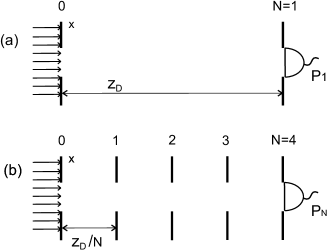
Figure 1: (a) Unobserved diffraction. (b) Observed diffraction.

Diffraction of the wave packet of envelope $\psi(x)$ by a slit of half-width $a$ can be described by the Fresnel diffraction integral, which is conveniently written in the form

$$\psi_{1}(\xi)=\frac{1}{\sqrt{2\pi i\zeta}}\int_{-1}^{1}d\xi^{\prime}\psi(\xi^{\prime})\exp\left[\frac{i}{2\zeta}(\xi^{\prime}-\xi)^{2}\right]\,,$$ (1)

where $\xi=x/a$ is the spatial coordinate in units of $a$, and $\zeta=z/(ka^{2})$ is the propagation distance $z$ in units of the diffraction distance $ka^{2}$, $k=2\pi/\lambda$ being the wave number and $\lambda$ the wavelength. Equation (1) describes also the spreading of the quantum wave packet of a particle $\psi(x)$ with center of mass at rest confined in $[-a,a]$ if $\zeta=\hbar t/(ma^{2})$ is the time $t$ in units of the diffraction time $ma^{2}/\hbar$.

In our numerical simulations, a uniform plane wave illuminates the slit (Fig. 1). The detector then measures the light power going through a slit of equal size placed at a fixed distance $\zeta_{\rm D}$, both when no slits are inserted (unobserved diffraction case) and when a number of intermediate slits are evenly inserted (observed diffraction case). Given $N$, $n=0,1,\dots N$ denote the source, intermediate, and detector slits at positions $\zeta_{n}=(\zeta_{\rm D}/N)n$. The number of intermediate slits is then $N-1$ (in particular, $N=1$ means no intermediate slits). In order to evaluate the field $\psi_{N}(\xi)$ at the detector slit and the captured power,

$$P_{N}=\int_{-1}^{1}|\psi_{N}(\xi)|^{2}d\xi\,,$$ (2)

we make use of Eq. (1) $N$ times with $\zeta=\zeta_{\rm D}/N$, starting with $\psi(\xi)={\rm const.}$ in $[-1,+1]$, to find the field in each intermediate slit from the preceding one until the detector slit. Figure 2(a) represents the power $P_{N}$ as a function of $N$, and shows that the detected power increases, though not monotonically, as more and more intermediate slits are inserted, approaching the power on the source slit, $P_{0}$, in the limit of large $N$. For $N=50$, for example, we get about 50% of power increase with respect to the case of no intermediate slits. Figure 2(b) shows that the eventual growth with large $N$ holds for all values of $\zeta_{\rm D}$. The detected power without intermediate slits (lower curve) is lower than the detected power with a large enough number of inserted slits (upper curves). Translated into a quantum mechanics language, we can affirm that a particle prepared in a localized state is more likely to preserve its localization if this property is checked a large enough number of times, since $P_{N}$ represents the probability of finding the particle in the localized region after $N$ measurements.

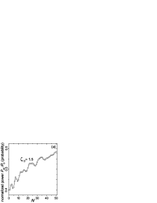
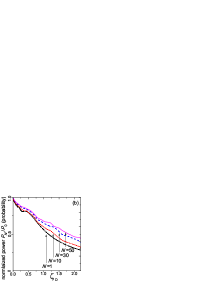
Figure 2: (Color online) Normalized power $P_{N}/P_{0}$ in the detector slit (a) as a function of the number of slits for a fixed source-detector distance $\zeta_{\rm D}$, and (b) as a function of the distance $\zeta_{\rm D}$ for a few, increasing number of slits within $\zeta_{\rm D}$.

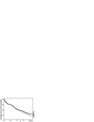
Figure 3: Normalized power $P(\zeta)/P_{0}$, where $P(\zeta)$ is computed according to Eq. (3), as a function of the propagation distance $\zeta$ for different number of intermediate slits within $\zeta_{\rm D}=2.0$. Steps are at $\zeta_{n}=n(\zeta_{\rm D}/N)$, $n=0,1\dots N$ for each $N$. The lowest step of each staircase is the power that arrives at the detector in each case.

Figure 3 illustrates how this Zeno effect is forged as light is diffracted more and more times in the intermediate slits. The power at a distance $\zeta$ is computed as

$$P(\zeta)=\int_{-\infty}^{\infty}|\psi_{\zeta}(\xi)|^{2}d\xi\,,$$ (3)

where $\psi_{\zeta}(\xi)$ represents the wave at plane $\zeta$. In absence of intermediate slits, the beam power is preserved (horizontal lighter line) until the beam impinges the detector slit, where it loses an important fraction of its power (vertical lighter line). As intermediate slits are inserted and their number increases, the “staircases” of power due to diffraction losses at each slit (darker lines) have more but so less steep steps that the power reaches higher and higher values at the detector. The same description applies to the probability of finding the particle after checking more and more frequently its presence in a finite region of space.

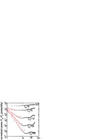
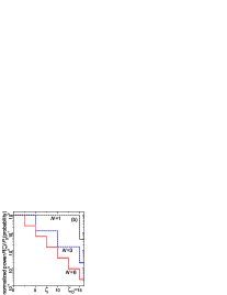
Figure 4: (Color online) (a) Open circles: Normalized power $P_{N}/P_{0}$ in the detector slit as a function of the number of intermediate slits for some given values of $\zeta_{\rm D}$. Dashed curves: prediction of Eq. (13), valid for $N\ll\zeta_{\rm D}$. (b) Solid curves: Normalized power $P(\zeta)/P_{0}$ as a function of the propagation distance $\zeta$ for different number of slits within $\zeta_{\rm D}=15$. The lowest step of each staircase is the power that arrives at the detector in each case. Dashed curves: the same but using the approximate values $(2N/\pi\zeta_{\rm D})^{n}$, $n=0,1\dots N$, at $\zeta_{n}=n(\zeta_{\rm D}/N)$.

As pointed out in the Introduction, a nonobvious fact is that the power in the detector starts to increase from the very first intermediate slit when the source-detector distance verifies $\zeta_{\rm D}\lesssim 2$ [see, for example, Fig. 2(a)]. The opposite situation with $\zeta_{\rm D}\gtrsim 2$ is illustrated in Fig. 4. Initially, inserting an increasing number of slits results in a regular decrease of the detected power [see Fig. 4(a), open circles curves], though the inclusion of further slits always reverses this trend. This is the more intuitive situation in which the more the loss events, the lower the power in the detector [Fig. 4(b), solid curves], and represents an anti-Zeno effect in wave-packet spreading: Repeated observation of wave-packet spreading within a certain distance or time $\zeta_{\rm D}$ enhances spreading compared to the unobserved case. The anti-Zeno effect is manifested when the observation intervals, or slit-to-slit distance, are slightly larger than one diffraction length: as seen in Fig. 4(a), the detected power at $\zeta_{\rm D}=5,10,15,20$ continuously decreases until $N=4,8,12,16$ slits, respectively, are inserted [Fig. 4(a)], which yields a slit-to-slit distance $\zeta_{\rm D}/N\simeq 1.25$ in all four cases. A similar value is obtained in other cases. The value $1.25$ times the diffraction length can be then considered as a Zeno distance (or time) in wave-packet spreading, which marks off the transition from a Zeno to an anti-Zeno behavior.

As a variant of the Zeno effect, the inverse-Zeno effect can also be observed in wave-packet spreading. The scheme of Fig. 1 is now changed by the one displayed in Fig. 5, where the detector slit is laterally displaced so that its bottom edge is at the same height as the top edge of the source slit, and therefore they do not overlap. As in the preceding cases, we insert equally spaced slits between the source and the detector, but they are now gradually displaced in the lateral direction by $\Delta\xi_{n}=n(2/N)$, $n=0,1\dots N$, as sketched in Fig. 5. The inverse-Zeno effect occurs if the light power reaching the detector in the observed diffraction case is larger than in the unobserved diffraction case, meaning that the wave has been guided by observation, at least partially, to the non-overlapping detector.

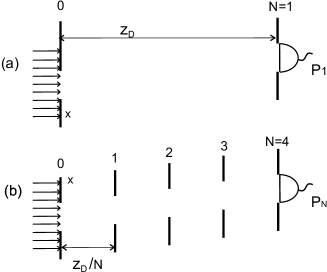
Figure 5: Scheme for the inverse-Zeno effect. (a) Unobserved diffraction. (b) Observed diffraction.

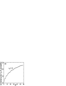
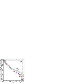
Figure 6: (Color online) For the inverse-Zeno scheme of Fig. 5, (a) normalized power $P_{N}/P_{0}$ on the detector slit as a function of the number of intermediate, laterally displaced slits for a fixed source-detector distance $\zeta_{\rm D}$; (b) normalized power $P(\zeta)/P_{0}$ as a function of the propagation distance $\zeta$ for different number of intermediate slits within $\zeta_{\rm D}$. Steps are at $\zeta_{n}=n(\zeta_{\rm D}/N)$, where the laterally displaced slits by $\Delta\xi_{n}=n(2/N)$, $n=0,1\dots N$ for each $N$ are placed. The lowest step of each staircase is the power that arrives at the detector in each case.

Figure 6(a) depicts the light power on the detector $P_{N}$ as a function of $N$ for given $\zeta_{\rm D}$, showing again a substantial rise with the number of intermediate, gradually displaced slits, a rise that reaches the source power $P_{0}$ in the limit $N\rightarrow\infty$. Figure 6(b) represents the power as a function of $\zeta$ for several number of intermediate, displaced slits within $\zeta_{\rm D}=1.5$. As described in relation to Fig. 3, light spreads between slits but preserves its power, experiencing therefore sudden drops as light impinges the intermediate slits. However, as in the Zeno effect, increasing the number of steps down results in a higher last step, that a higher detected power. In the analogous quantum mechanical system, the particle can be said to be guided to the desired region of space by repeatedly asking the particle if it is gradually displaced toward that region. As in the Zeno effect, this inverse-Zeno effect is preceded by an inverse-anti-Zeno effect when the source-detector distance allows low enough frequency of the measurements.

III Theory

To simplify the notation and emphasize the parallelism with quantum mechanics, we rewrite the Fresnel integral in Eq. (1) as

$$\psi_{1}(\xi)=U(\zeta)\psi_{0}(\xi)\,,$$ (4)

where $\psi_{0}(\xi)=T(\xi)\psi(\xi)$ is the initial localized state due to truncation with the aperture function

$$T(\xi)=\left\{\begin{array}[]{ll}1&\mbox{if}\quad|\xi|\leq 1\\ 0&\mbox{otherwise}\end{array}\right.\,,$$ (5)

and where $U(\zeta)=\exp(-iH\zeta)$ is the evolution operator, with $H=-\frac{1}{2}\partial^{2}/\partial\xi^{2}$ the Hamiltonian. Setting

$$P_{0}=\int d\xi|\psi_{0}(\xi)|^{2}=1\,,$$ (6)

all expressions below hold equally for the quantum probability or the light power normalized to the source power.

III.1 One-dimensional Zeno effect

In a standard Zeno scheme, measurements check whether the evolved state $U(\zeta)|\psi_{0}\rangle$ is in the initial localized state $|\psi_{0}\rangle$. Measurement is described by applying the projector $|\psi_{0}\rangle\langle\psi_{0}|$ to $U(\zeta)|\psi_{0}\rangle$, so that the emerging state is $|\psi_{0}\rangle\langle\psi_{0}|U(\zeta)|\psi_{0}\rangle$ and the probability of finding the initial state is given by $|\langle\psi_{0}|U(\zeta)|\psi_{0}\rangle|^{2}$. Applying this scheme to $N$ measurements evenly spaced by $\zeta_{\rm D}/N$ in $\zeta_{\rm D}$, the probability of finding the initial state $|\psi_{0}\rangle$ in the last measurement is $P_{N}^{(S)}=|\langle\psi_{0}|U(\zeta_{\rm D}/N)|\psi_{0}\rangle|^{2N}$, or

$$P_{N}^{(S)}=\left|\int d\xi\psi_{0}^{\star}(\xi)U(\zeta_{\rm D}/N)\psi_{0}(\xi)\right|^{2N}\,,$$ (7)

where the superscript $(S)$ stands for “standard” scheme. The probability is the product of individual probabilities because the state is reset, except for its amplitude, to the initial state in each measurement. In the standard Zeno, $U$ is usually approached by $U=1+iH(\zeta_{\rm D}/N)+(1/2)H^{2}(\zeta_{\rm D}/N)^{2}$ for large-enough $N$. Further, in case that $\langle\psi_{0}|H|\psi_{0}\rangle$ and $\langle\psi_{0}|H^{2}|\psi_{0}\rangle$ are well-defined, $P_{N}^{(S)}\simeq\left[1-\left(\zeta_{\rm D}/N\right)^{2}(\Delta H)^{2}_{\psi_{0}}\right]^{N}\rightarrow 1$ as $N\rightarrow\infty$ is obtained, meaning that the state is $|\psi_{0}\rangle$ in the limit of infinitely frequent measurements.

III.2 Zeno effect within a subspace in wave-packet spreading

In Sec. II we instead have checked if the position of the quantum particle remains in the initial space domain $[-1,+1]$. A measurement is then described by applying the projector $\int_{-1}^{+1}d\xi|\xi\rangle\langle\xi|$, the state after the measurement then being $\int_{-1}^{+1}d\xi|\xi\rangle\langle\xi|U(\zeta)|\psi_{0}\rangle$, or $T(\xi)U(\zeta)\psi_{0}(\xi)$ in position representation. Accordingly, the state after $N$ measurements of position within $\zeta_{\rm D}$ is

$$\psi_{N}(\xi)=T(\xi)U(\zeta_{\rm D}/N)\cdots T(\xi)U(\zeta_{\rm D}/N)\psi_{0}(\xi)\,,$$ (8)

and the probability of finding the particle in $[-1,+1]$ is

$$P_{N}=\int d\xi|T(\xi)U(\zeta_{\rm D}/N)\cdots T(\xi)U(\zeta_{\rm D}/N)\psi_{0}(\xi)|^{2}\,.$$ (9)

As explained, this quantum dynamics is analogous to that of repeated diffraction in a distance $\zeta_{\rm D}$, $P_{N}$ then meaning the power in the $N$th slit normalized to the power on the source slit. Generally, it is not possible to factorize Eq. (9) as in the standard Zeno scheme, since the state is not reset to the initial one in each measurement, and other approaches must be pursued to explain the Zeno and anti-Zeno effects described in Sec II.

III.2.1 Fraunhofer regime

Let us first analyze the anti-Zeno effect. Suppose that $\zeta_{\rm D}$ is large enough, and $N$ is small enough that the slit-to-slit distance $\zeta_{\rm D}/N\gg 1$. For the input square wave $\psi_{0}(\xi)=T(\xi)/\sqrt{2}$ considered in the preceding section, we have

$$U(\zeta_{D}/N)\psi_{0}(\xi)\simeq\frac{e^{i\xi^{2}N/2\zeta_{\rm D}}}{\sqrt{2}}\left(\frac{2N}{\pi i\zeta_{\rm D}}\right)^{1/2}\frac{\sin(\xi N/\zeta_{\rm D})}{\xi N/\zeta_{\rm D}}\,,$$ (10)

where Fraunhofer diffraction has been used. Well within the Fraunhofer region ($\zeta_{\rm D}/N\gg 1$), this pattern can be regarded as approximately uniform in the limited region $[-1,+1]$, and thus we write

$$\psi_{1}(\xi)=T(\xi)U(\zeta_{\rm D}/N)\psi_{0}(\xi)\approx\frac{T(\xi)}{\sqrt{2}}\left(\frac{2N}{\pi i\zeta_{\rm D}}\right)^{1/2}$$ (11)

for the wave just after the first slit, with power $(2N/\pi\zeta_{\rm D})$. Within this approximation, we can repeatedly apply the operator $T(\xi)U(\zeta_{\rm D}/N)$ to obtain similar expressions for the wave $\psi_{n}(\xi)$ just after the $n$th slit, and its power as $(2N/\pi\zeta_{\rm D})^{n}$. In particular, the wave on the detector is

$$\psi_{N}(\xi)\approx\frac{T(\xi)}{\sqrt{2}}\left(\frac{2N}{\pi i\zeta_{\rm D}}\right)^{N/2}\,,$$ (12)

and the measured power is

$$P_{N}\approx\left(\frac{2N}{\pi\zeta_{\rm D}}\right)^{N}\,.$$ (13)

Given $\zeta_{\rm D}$, this expression is expected to be approximately valid for $N\ll\zeta_{\rm D}$. The value of $P_{N}$ given by Eq. (13) is seen to be a decreasing function of $N$ for $N\ll\zeta_{\rm D}$ [Fig. 4(a), dashed curves] that provides an accurate description of the anti-Zeno effect in wave-packet spreading. The power loss by repeated factors $(2N/\pi\zeta_{\rm D})$ gives a good description of the actual power loss as light impinges each intermediate slit during its propagation from the source to the detector [Fig. 4(b), dashed curves].

III.2.2 Fresnel regime

The anti-Zeno effect disappears when the slit-to-slit distance is not in the Fraunhofer region. With increasing number of slits, diffraction can act a sufficient number of times to shape a diffraction wave mode, whose much lower diffraction losses can explain the Zeno effect described in Sec. II. As originally studied for plane, two-mirror (Fabry-Perot) resonators FL , a diffraction mode self-reproduces upon propagation from one to the next diffracting slit (from mirror to mirror) apart from a complex constant or eigenvalue, that is, $\psi_{n+1}(\xi)=\gamma\psi_{n}(\xi)$. Accordingly, the power varies as $P_{n+1}=|\gamma|^{2}P_{n}\equiv(1-\delta)P_{n}$, where $\delta$ is the fractional power loss per slit (i.e., per mirror reflection). The shape of a diffraction wave mode and its fractional power loss depend on the slit spacing (mirror distance) $L$. For the fundamental diffraction mode the fractional power loss can be approximated by $\delta\approx 0.12N_{F}^{-3/2}$ if the resonator Fresnel number $N_{F}=a^{2}/(\lambda L)$ is greater than unity FL .

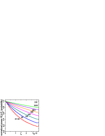
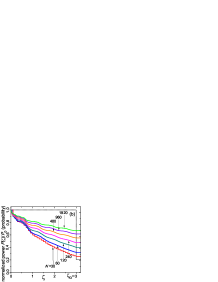
Figure 7: (Color online) Normalized power $P(\zeta)/P_{0}$ as a function of the propagation distance $\zeta$ for different large numbers of intermediate slits within $\zeta_{\rm D}=3.0$ (a) as predicted by the model of diffraction modes, and (b) evaluated as in Fig. 3 starting with uniform illumination.

For a large-enough number of intermediate slits between the source and the detector, we can assume that the diffraction mode corresponding to the slit spacing propagates from slit to slit and apply the above theory. In our case, the slit spacing is $L=z_{\rm D}/N$, the Fresnel number is $N_{F}=Na^{2}/\lambda z_{\rm D}$, or, in our dimensionless variables, $N_{F}=N/2\pi\zeta_{\rm D}$, and the fractional power loss per slit becomes $\delta=b(\zeta_{\rm D}/N)^{3/2}$ [$b=0.12(2\pi)^{3/2}\simeq 1.8899$]. Thus, as the number of slits $N$ increases, the Fresnel number increases proportionally, but the losses per slit decrease as the faster rate $N^{-3/2}$, which results in a higher power on the detector. More precisely, the variation of the power from slit to slit is given by $P_{n+1}-P_{n}=-b(\zeta_{\rm D}/N)^{3/2}P_{n}$, which leads, for small slit spacing, to the exponential decay

$$P_{n}\simeq P_{0}\exp\left[-b\left(\frac{\zeta_{\rm D}}{N}\right)^{1/2}\zeta_{n}\right]\,,$$ (14)

with a “life-time” growing as $N^{1/2}$. In particular, the power on the detector $P_{N}=P_{0}\exp\left(-b\zeta_{\rm D}^{3/2}/N^{1/2}\right)$ also increases as $N^{1/2}$, approaching $P_{0}=1$ as $N\rightarrow\infty$. The exponentially decaying steps of the power for different, large numbers of intermediate slits, as predicted by Eq. (14), are represented in Fig. 7(a) in order to show that this simple model reproduces the mechanism of the actual Zeno effect, represented in Fig. 7(b). These two figures differ quantitatively because in (a) the fundamental diffraction mode is assumed to propagate from the beginning, while in (b) the diffraction mode is gradually formed from the input uniform illumination. Figure 8 shows the gradual formation of the diffraction mode (thick solid curve) as the input square wave is diffracted by the successive slits for $N=480$ slits in $\zeta_{\rm D}=3$, corresponding to a slit spacing $0.00625$ and a Fresnel number $N_{F}\simeq 25.5$ (as an example, for visible light at $\lambda=600$ nm and a slit of width $2a=1$ mm, three diffraction lengths would be 7854 mm and the slit spacing would be about $16.36$ mm). The process of mode formation from the uniform illumination causes the decays in Fig. 7(b) to be initially faster than exponential, but they are moderated to the same exponential decays as in Fig. 7(a) at distances where the wave mode is substantially formed. The result is a slightly less pronounced Zeno effect in the detected power compared to the prediction of the simple model starting with diffraction modes. Also, the uniform illumination excites spurious higher-order diffraction modes. Since their diffraction losses are higher, the oscillations observed in Fig. 7(b) and caused by interference with the fundamental mode, attenuate with propagation distance.

The inverse-Zeno effect with misaligned slits can be understood from the diffraction mode theory in a similar way as the Zeno effect. The only significant difference is that the diffraction wave mode that builds up by repeated diffraction and the corresponding losses per slit, are those of a misaligned, two-mirror laser resonator, as described in specific studies on the effects of misalignment on these resonators FL .

Figure 8: Solid curve: amplitude $|\psi(\xi)|$ of the fundamental diffraction mode for $N_{F}\simeq N/(2\pi\zeta_{\rm D})\simeq 25.5$, corresponding to $N=480$ slits in $\zeta_{\rm D}=3$. Dashed curves: amplitudes $|\psi_{n}(\xi)|$ on the intermediate slits $n=0,40,80$ showing the gradual formation of the fundamental diffraction mode explaining the Zeno effect. For better comparison, all peak amplitudes are normalized to unity.

IV Conclusions

We have analyzed a simple and feasible scheme displaying Zeno, anti-Zeno, and inverse-Zeno effects, valid in quantum mechanics and classical wave optics. The classical wave optics scheme is particularly simple since observation of the system is achieved just by inserting slits between a light source and a light-power detector.

We have shown that the occurrence of Zeno or anti-Zeno effect depends on the separation between the source and the detector and the number of intermediate slits. The anti-Zeno effect seems more intuitive: Adding diffracting slits increases diffraction and holds for large enough separation between slits (i.e., less frequent measurements). This separation is close to the diffraction length (which is determined by slit size and light wavelength). On the other hand, the Zeno effect holds for smaller separation between slits (i.e., more frequent measurements) and corresponds to the rather counterintuitive behavior that diffraction is inhibited by placing more and more diffracting slits between the source slit and the detector. The slit separation for the transition between Zeno and anti-Zeno effects is the analog of the so-called Zeno time Lane83 ; Schieve89 ; Kofman96 ; Alfredo98 ; Maniscalco06 ; Francica10 .

We have related the Zeno effect to the diffraction mode theory in Fabry-Perot resonators. The total power losses during passage through tightly space slits are less than the total losses through widely spaced slits within the same distance. This is because a diffraction mode of the equivalent resonator tends to be formed by the many diffractions and because the mode losses are lower as the slit spacing diminishes. In this regard, the limit of a continuous of measurements in the quantum domain has been considered in Ref. Fakki ; rev , where it is shown that the wave packet evolves as in an infinitely deep well potential. In classical wave optics, such an ideal limit might be regarded as a perfect conductor waveguide forcing the vanishing of the electric field at its walls, avoiding diffraction losses by expelling the field away from the walls.

References

- eprint
- (1) B. Misra and E. C. G. Sudarshan, J. Math. Phys. 18, 756 (1977).
- (2) L. A. Khalfin, Zh. Eksp. Teor. Fiz. 33, 1371 (1957) [Sov. Phys. JETP 6, 1053 (1958)]; R. G. Winter, Phys. Rev. 123, 1503(1961); W. Yourgrau, in Problems in the Philosophy of Science, edited by I. Lakatos and A. Musgrave (North-Holland, Amsterdam, 1968), pp. 191-192.
- (3) W. M. Itano, D. J. Heinzen, J. J. Bolinger, and D. J. Winelad, Phys. Rev. A 41, 2295 (1990).
- (4) J. G. Muga, J. Echanobe, A. del Campo, and I. Lizuain, J. Phys B 41, 175501 (2008).
- (5) A. M. Lane, Phys. Lett. A 99, 359 (1983).
- (6) W. C. Schieve, L. P. Horwits, and J. Levitan, Phys. Lett. A 136, 264 (1989).
- (7) A. G. Kofman and G. Kurizki, Phys. Rev. A 54, R3750 (1996); A. G. Kofman and G. Kurizki, Nature (London) 405, 546 (2000).
- (8) A. Luis and L. L. Sánchez-Soto, Phys. Rev. A 57, 781 (1998).
- (9) S. R. Wilkinson, C. F. Bharucha, M. C. Fischer, K. W. Madison, P. R. Morrow, Q. Niu, B. Sundaram, and M. G. Raizen1, Nature (London) 387, 575 (1997).
- (10) M. C. Fischer, B. Gutiérrez-Medina, and M. G. Raizen, Phys. Rev. Lett. 87, 040402 (2001).
- (11) F. Dreisow, A. Szameit, M. Heinrich, T. Pertsch, S. Nolte, A. Tuünnermann, and S. Longhi, Phys. Rev. Lett. 101, 143602 (2008).
- (12) I. Lizuain, J. Casanova, J. J. García-Ripoll, J. G. Muga, and E. Solano, Phys. Rev. A 81, 062131 (2010)
- (13) M. Kitano, Opt. Commun. 141, 39 (1997).
- (14) K. Yamane, M. Ito, and M. Kitano, Opt. Commun. 192, 299 (2001).
- (15) Y. Aharonov and M. Vardi, Phys. Rev. D 21, 2235 (1980).
- (16) T. P. Altenmüller and A. Schenzle, Phys. Rev. A 48, 70 (1993).
- (17) A. Peres, Am. J. Phys. 48, 931 (1980); P. Kwiat, H. Weinfurter, T. Herzog, A. Zeilinger, and M. Kasevich, Ann. NY Acad. Sci. 755, 383 (1995).
- (18) S. Longhi, Phys. Rev. Lett. 97, 110402 (2006).
- (19) P. Biagioni, G. Della Valle, M. Ornigotti, M. Finazzi, L. Duo, P. Laporta, and S. Longhi, Opt. Express 16, 3762 (2008).
- (20) M. Moshinsky, Phys. Rev. 88, 625 (1952); E. Torrontegui, J. Muñoz, Y. Ban, and J. G. Muga Phys. Rev. A 83, 043608 (2011).
- (21) A. G. Fox and T. Li, Bell Syst. Tech. J. 40, 453 (1961); A. E. Siegman, Lasers (University Science Books, South Orange, NJ, 1986).
- (22) P. Facchi, V. Gorini, G. Marmo, S. Pascazio, and E.C.G. Sudarshan, Phys. Lett. A 275, 12 (2000); P. Facchi, S. Pascazio, A. Scardicchio, and L. S. Schulman, Phys. Rev. A 65, 012108 (2001); P. Facchi, G. Marmo, S. Pascazio, A. Scardicchio, and E. C. G. Sudarshan, J. Opt. B: Quantum Semiclass. Opt. 6, S492 (2004).
- (23) P. Facchi and S. Pascazio, Phys. Rev. Lett. 89, 080401 (2002); J. Phys. A: Math. Theor. 41 493001 (2008); M. V. Berry and S. Klein, J. Mod. Opt 43, 2139 (1996); M. V. Berry, in The Mathematical beauty of Physics, edited by J.-M. Drouffe and J.-B. Zuber (World Scientific, Singapore, 1997), pp. 281-294; M. V. Berry, J. Phys. A 29, 6617 (1996); M. V. Berry, I. Marzoli, and W. Schleich, Phys. World 14(6), 39 (2001).
- (24) S. Maniscalco, J. Piilo, and K.-A. Suominen, Phys. Rev. Lett. 97, 130402 (2006).
- (25) F. Francica, F. Plastina, and S. Maniscalco, Phys. Rev. A 82, 052118 (2010).