A Solvable Model for Polymorphic Dynamics of Biofilaments

Abstract

We investigate an analytically tractable toy model for thermally induced polymorphic dynamics of cooperatively rearranging biofilaments - like microtubules. The proposed 4 -block model, which can be seen as a coarse-grained approximation of the full polymorphic tube model, permits a complete analytical treatment of all thermodynamic properties including correlation functions and angular fourier mode distributions. Due to its mathematical tractability the model straightforwardly leads to some physical insights in recently discussed phenomena like the ”length dependent persistence length”. We show that a polymorphic filament can disguise itself as a classical wormlike chain on small and on large scales and yet display distinct anomalous tell-tale features indicating an inner switching dynamics on intermediate length scales.

I Introduction

Biological filaments of the cytoskeleton are large macromolecules formed by a hierarchical self-assembly of smaller yet often highly complex protein subunits. The monomer complexity can allow the subunits to undergo rearrangements between several conformational states. Once inserted into a macromolecular lattice these individual subunits can start to interact giving rise to cooperative phenomena which can affect equilibrium and dynamical properties of the whole assembly in unexpected manners. It is the goal of this paper to explore in detail the statistical mechanics of this type of cooperatively switching supramolecular assemblies, whose paradigm example might be found in the stiffest cytoskeletal protein filaments of eukaryotic cells, the microtubules Alberts . Microtubules are hollow nanotubes whose walls are formed by lateral self-association of parallel protofilaments that themselves are built by a head-to-tail polymerization of $\alpha\beta$-tubulin heterodimer protein subunits. This very complex architecture confers to microtubules their high stiffness as well as a number of unique static and dynamic properties. In MTKulic1 , guided by experimental findings, we built the case for a novel model of microtubules, based on two hypotheses: the elementary tubulin dimer units can fluctuate between a curved and a straight configuration and can interact cooperatively along a protofilament axis. This implies that the ground state of microtubules is not, as usually accepted a straight Euler beam, but instead a fluctuating several micron sized cooperative super-helix. The resulting polymorphic dynamics of the microtubule lattice seems to quantitatively explain several experimental puzzles including anomalous scaling of dynamic fluctuations of grafted microtubules Taute , their apparent length-stiffness relation Pampaloni and their remarkably curved-helical appearance in general Venier . These results rely on phenomenological modelling where the cylindrical symmetry of the microtubule lattice is approximated by a continuous symmetry MTKulic1 . This approximation seems reasonable as the number of protofilaments is typically large, ranging from $9$ to $17$ for taxol stabilized in-vitro microtubules with a predominant $14$ protofilament structure Wade ; Chretien . In vivo, microtubules most commonly appear with $13$ protofilaments Bouchet , although many exceptions exist depending of the cell type. The approach developed in MTKulic1 revealed the existence of a unique and unusual zero mode dynamics which has strong consequences : microtubules are permanently coherently reshaping -i.e. changing their reference ground state configuration- by thermal fluctuations.

Going beyond the continuous phenomenological approach of MTKulic1 , we explore here other important aspects of the polymorphic microtubules theory by considering a simplified minimal solvable model. We will adopt a coarse-grained approach where the microtubule lattice is considered as made up of only $4$ blocks of protofilaments that can fluctuate between a curved and a straight configuration. Although the coarse-grained model to some extent loses the (quasi)continuous zero mode dynamics, it captures a number of important features of the full model MTKulic1 and exact analytic computations of relevant observables becomes accessible in this simpler case. In particular the tubulin-tubulin state correlation function, the persistence length, the thermodynamic stability of conformational states as well as the tangent angle spectrum can be computed rather elegantly. This simplified approach should give more detailed analytical insights into microtubule’s static properties and make connection with the previous phenomenological model’s parameters introduced in MTKulic1 . While it is not our prime goal here to compare the developed toy model with experiments we hope that some of the derived results (like the tangent angle power spectrum) can become useful guides for future experimental quantification of polymorphic filament fluctuations. For a more detailed experiment-theory comparison and deeper motivation of the model we refer the reader to the articles MTKulic1 .

II The 4-block polymorphic tube model

The microtubule lattice (see Fig. 1) is modelled as a continuum tube material made of a variable number of protofilaments with $R_{i}\approx 7.5nm,$ $R_{o}\approx 11.5nm$ - the inner and outer microtubule radii respectively. The protofilaments are twisted around the microtubule’s longitudinal axis with the corresponding internal twist $q_{0}$ - or equivalently the pitch $\lambda=2\pi q_{0}^{-1}$ - being a lattice type dependent constant that takes typical discrete values $\lambda=+3.4\mu m,+25\mu m,-6\mu m$ for $12$, $13$ and $14$ protofilament microtubules respectively Wade ; Chretien Ray ChretienFuller .

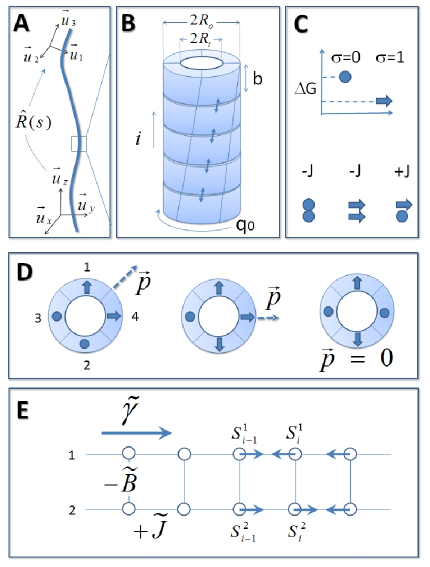
Figure 1: Elements of the ”polymorphic four block tube model”. (a) Tube contour with the internal and external frames. (b) A short tube section with intrinsic twist $q_{0}$ with four blocks at each section. (c) The blocks can fluctuate cooperatively between two discrete states. The outwards curved $\sigma=1$ (arrow) state is energetically preferred over the straight state $\sigma=0$ (circle) with an energy gain $E=-\Delta G$. The junction between straight and curved states along the longitudinal block axis are penalized by a coupling constant $E=+J.$ (d) Competition between block switching energy and elastic lattice strain energy leads to spontaneous symmetry breaking: the tube bends to a randomly chosen direction and assumes a non-zero vectorial polymorphic order parameter $\vec{p}$ (”conformational polarization”) (e) The four block model can be decoupled into a pair of two-block models which can be mapped onto a ladder type Ising model with coupling constants $-\widetilde{B}$ and $+\widetilde{J}$ and a bias field $\widetilde{\gamma}$.

To describe the tube’s geometry we introduce two reference frames (cf. Fig. 1A). One is the material frame with base vectors $(\vec{u}_{1},\vec{u}_{2},\vec{u}_{3})$ attached to each microtubule cross-section. The other is an external fixed laboratory frame with base vectors $(\vec{u}_{x},\vec{u}_{y},\vec{u}_{z})$ with respect to which all deformations are measured. Putting the filament along the $\vec{u}_{z}$ axis direction and considering small angular deflections we have $\vec{u}_{z}\approx\vec{u}_{3}$. In this case the two frames are simply related by a rotation transformation $\hat{R}(s)$ given by internal microtubule lattice twist $q_{0}$, such that $(\vec{u}_{x},\vec{u}_{y})=\hat{R}(s)(\vec{u}_{1},\vec{u}_{2})$ with

$$\hat{R}(s)=\left(\begin{array}[c]{cc}\cos(q_{0}s+\varphi)&-\sin(q_{0}s+\varphi)\\ \sin(q_{0}s+\varphi)&\cos(q_{0}s+\varphi)\end{array}\right)$$ (1)

and $s\in\left[0,L\right]$ the longitudinal position variable along the microtubule centerline. The arbitrary rotation angle $\varphi$ corresponds to the angular deviation between the two frames at $s=0.$ As each protofilament is built by a self association of $N$ discrete GDP-tubulin dimers of length $b\approx 8nm$ it is natural to introduce a discrete variable $i$ such that all microtubule’s cross-section positions are written as $s=ib$ with $i=1..N.$

The coarse-grained block approximation consists of grouping neighboring protofilaments into $n=4$ effective blocks (cf. Fig. 1B). The fluctuations of the block-dimers between 2 states - a straight and a curved state with intrinsic curvature $\kappa_{FP}$ and with an energy difference $\Delta G>0$ favoring the curved state are modelled by a two state variable $\sigma_{i}^{k}=0,1$ where $i=1..N$ is the longitudinal position and $k=1..4$ the block’s index (cf. Fig. 1C).

To complete the description of the polymorphic tube model two order parameters at each microtubule cross-section can be introduced MTKulic1 . The first is the vectorial polymorphic order parameter $\vec{p}_{i}=\vec{u}_{1}(\sigma_{i}^{1}-\sigma_{i}^{2})+\vec{u}_{2}(\sigma_{i}^{4}-\sigma_{i}^{3}),$ a 2D vector attached to each cross-section (cf Fig. 1D) describing the asymmetry of the curved state distribution - a kind of ”conformational polarization vector” of the block states. For instance the ”all-straight” or ”all-curved” protofilament state correspond both to the same value $\vec{p}=0$, cf. Fig. 1D (as the curved state distribution is isotropic in both special cases). A second (scalar) quantity $m_{i}=\sum_{k=1}^{4}\sigma_{i}^{k}$ counts the total number of blocks in the curved state at each cross-section $i$. The tubulin cooperativity along each protofilament (block) axis is modelled by an Ising type nearest-neighbor cooperative interaction with an interaction energy $J>0$ favoring longitudinal nearest neighbors to be in the same state. The interaction energy at cross-section $i$ reads:

$$e_{inter,i}=-J\sum\nolimits_{k=1}^{4}\left(2\sigma_{i}^{k}-1\right)\left(2\sigma_{i+1}^{k}-1\right)$$ (2)

The total elastic + polymorphic energy can then be written as MTKulic1 :

$$E_{MT}=\sum\nolimits_{i=1}^{N}\left(e_{i}+e_{inter,i}\right).$$ (3)

where $e_{i}$ is the combined elastic energy and the energy resulting from the switching of tubulin dimers at i-th cross-section:

$$e_{i}=\frac{Bb}{2}\left[\left(\vec{\kappa}_{i}-\vec{\kappa}_{pol,i}\right)^{2}+\frac{\kappa_{1}^{2}}{2}\left(\frac{\pi\gamma}{2}m_{i}-p_{i}^{2}\right)\right]$$ (4)

with the elastic bending modulus $B=\frac{Y\pi}{4}\left(R_{o}^{4}-R_{i}^{4}\right)$ and $Y$ the Young modulus. The effective lattice curvature $\kappa_{1}=\frac{\left(R_{0}-R_{1}\right)^{2}}{\pi\left(R_{o}^{2}+R_{i}^{2}\right)}\kappa_{FP}$ results directly from the preferred curvature of the individual protofilament $\kappa_{PF}$ MTKulic1 . Here $\vec{\kappa}$ is the microtubule centerline curvature vector and $\vec{\kappa}_{pol}$ the polymorphic curvature vector which in the external coordinate frame $\left(\vec{u}_{x},\vec{u}_{y}\right)$ is

$$\vec{\kappa}_{pol,i}=2^{-1/2}\kappa_{1}\hat{R}(ib)\vec{p}_{i}$$ (5)

In Eq. 4 we introduced an important dimensionless parameter $\gamma=\frac{\kappa_{PF}}{\kappa_{1}}-\frac{8\Delta G}{bB\kappa_{1}^{2}}$ which measures the competition between block switching and elastic energy and ultimately determines the microtubule shape. It effectively acts as an external field that biases the curved lattice state for $\gamma<0$ and favors the straight state for $\gamma>0$ (cf. below). For small deflections $\theta_{x/y}<<1$ around the $z$-axis, the unit vector tangent to the microtubule’s centerline is approximately given by $\vec{t}\approx(\theta_{x},\theta_{y},1)$ in the laboratory frame $\left(\vec{u}_{x},\vec{u}_{y},\vec{u}_{z}\right)$ where $\vec{\theta}=\left(\theta_{x},\theta_{y}\right)$ are the centerline deflection angles in x/y direction. The global centerline curvature vector $\vec{\kappa}=d\vec{t}/ds$ can then be approximated as $\overrightarrow{\kappa}\approx\left(\theta_{x}^{\prime},\theta_{y}^{\prime},0\right).$ Writing the total curvature as $\overrightarrow{\kappa}=\overrightarrow{\kappa}_{pol}+\overrightarrow{\theta^{\prime}}_{el}$ with $\overrightarrow{\theta^{\prime}}_{el}$ the purely elastic contribution we readily see from Eqs. 2,3 that the partition function decomposes into a product of two independent elastic and polymorphic contributions $Z=Z_{el}Z_{pol},$ with $Z_{el}=\int D\theta\exp\left(-\frac{l_{B}}{2}\int\nolimits_{0}^{L}\theta_{el}^{\prime 2}ds\right)$ (and $l_{B}=B/k_{B}T$ the bending persistence length with $k_{B}T$ the thermal energy). Therefore our main goal reduces to the computation of $Z_{pol}=\sum_{\sigma}\exp(-\frac{1}{k_{B}T}E_{\sigma})$ with $E_{\sigma}$ the polymorphic contribution of $E_{MT}$. In the general case (with large number of blocks) this appears to be a formidable task, that however can be exactly performed in the case of $4$ blocks as we will see in the following.

II.1 Reduction to a 2 $\times$ 2-block model

We first note that, at each cross-section $p_{i}^{2}=\left(\sigma_{i}^{4}-\sigma_{i}^{3}\right)^{2}+(\sigma_{i}^{2}-\sigma_{i}^{1})^{2}$ decomposes into a sum over mutually facing blocks i.e. only blocks 1-2 and 3-4 couple directly. Consequently the partition function can be factorized into a product of two simpler ones $Z_{pol}=Z_{12}Z_{34}$ with $Z_{kl}$ the partition function of the Ising variables $\sigma^{k}$ and $\sigma^{l}$ of the blocks that face each other, cf. Fig. 1D. Therefore from now on we may consider the $2$ block model, say the block pair $1-2$. The polymorphic order parameters are in this case $m_{i}=\sigma_{i}^{1}+\sigma_{i}^{2}$ and $\overrightarrow{p}_{i}=\left(\sigma_{i}^{1}-\sigma_{i}^{2}\right)\vec{u}_{1}.$ By introducing new more convenient Ising variables $S_{i}^{k}=\pm 1$ defined as $S_{i}^{k}=2\sigma_{i}^{k}-1$ the energy Eq. 2 takes the familiar form of a ladder type Ising model (cf. Fig. 1E). In terms of these variables, $Z_{12}=Z_{0}\widetilde{Z}$ with $Z_{0}=\exp(\frac{1}{k_{B}T}B\kappa_{1}^{2}L\left(\pi\gamma-1\right)/4)$ and

$$\widetilde{Z}=\sum_{\left\{S^{1},S^{2}\right\}=-1,1}\exp(-\widetilde{E})$$ (6)

where from Eqs. 2-4 we obtain

$$\widetilde{E}={\textstyle\sum_{i=1}^{N}}\left[\widetilde{B}S_{i}^{1}S_{i}^{2}+\widetilde{\gamma}\left(S_{i}^{1}+S_{i}^{2}\right)-\widetilde{J}\left(S_{i}^{1}S_{i+1}^{1}+S_{i}^{2}S_{i+1}^{2}\right)\right]$$ (7)

with $\widetilde{B}=\frac{B\kappa_{1}^{2}b}{4k_{B}T},$ $\widetilde{J}=\frac{J}{k_{B}T}$ and $\widetilde{\gamma}=\frac{\pi}{2}\gamma\widetilde{B}.$ With the two spins - on either side of the ladder (Fig. 1E)- being interchangeable we have $\left\langle S_{i}^{1}\right\rangle=\left\langle S_{i}^{2}\right\rangle$ (and thus $\left\langle\sigma_{i}^{1}\right\rangle=\left\langle\sigma_{i}^{2}\right\rangle$) for all $i$ as the energy is translationally invariant. From Eq. 5, we readily see that $\left\langle\vec{\kappa}_{pol,i}\right\rangle=0.$ And yet this does not mean that the microtubule is on average in a straight configuration. Just on the contrary, the microtubule can form a three dimensional super helix MTKulic1 that is ”coherently” reshaping as the curvature alternately exchanges from one block to the other with a non-vanishing value of $\left\langle\kappa_{pol}^{2}\right\rangle$. Therefore the order parameter that characterizes the typical curvature of the lattice is the mean ”polarization” $P=\sqrt{N^{-1}\sum_{i}\left\langle\overrightarrow{p}_{i}^{2}\right\rangle}$ of the curved states (as $\left\langle\kappa_{pol}^{2}\right\rangle=\kappa_{1}^{2}P^{2}$). The other important quantity is $M=\frac{1}{N}\sum\nolimits_{i}\left\langle\sigma_{i}^{k}\right\rangle=\left\langle\sigma_{i}^{k}\right\rangle$ - the mean concentration of curved states, or in the Ising terminology the mean ”magnetization” (up to a trivial additive constant) . Within the same terminology the parameter $\widetilde{\gamma}$ takes the role of a ”magnetic field” that, according to its sign, favors one or the other possible spin orientation (curved or straight block) -but the same orientation for blocks on both sides of the ladder in Fig. 1E. The ”ferromagnetic coupling constant ” $\widetilde{J}$ promotes the longitudinal parallel alignments of spins along a given block axis. The ”anti-ferromagnetic coupling” $\widetilde{B}$ on the other hand favors $S_{i}^{1}$ and $S_{i}^{2}$ to be antiparallel - a tendency which competes with $\widetilde{\gamma}$ and the lattice is frustrated. For large $\left|\widetilde{\gamma}\right|>>\widetilde{B}$, we therefore expect the alignment tendency to win on both sides of the ladder so that $\left\langle S_{i}^{1/2}\right\rangle\approx\pm 1,$ ($+1$ if $\widetilde{\gamma}<0$ and $-1$ if $\widetilde{\gamma}>0$) and thus $M\approx 1$ or $0.$ In this situation the microtubule is in a straight state with $P\approx 0$, which is either completely unstressed with $M\approx$ $0$ (for positive $\widetilde{\gamma}$) or maximally prestrained state with $M\approx 1$ (for negative $\widetilde{\gamma}$).

For $\widetilde{\gamma}=0,$ the lattice is not frustrated and on average when on one ladder-side $S_{i}^{1}=1$ then $S_{i}^{2}=-1$ on the other (and vice versa). Consequently $\left\langle S_{i}^{k}\right\rangle=0$ and $M=\left\langle\sigma_{i}^{k}\right\rangle=1/2.$ In this case blocks $1$ and $2$ at the cross-section $i$ fluctuate alternately between the curved and straight state and the tube bends alternately in the directions $\vec{u}_{1}$ and $-\vec{u}_{1}.$ The cooperative ferromagnetic interaction $\widetilde{J}$ implies a correlation between the spins along the contour and the formation of domains with size of the order of the spin-spin correlation length $\xi$ computed below. It is these whole domains that alternately bend the tube in the $\vec{u}_{1}$ and $-\vec{u}_{1}$ direction that lead to $\left\langle\overrightarrow{p}_{i}\right\rangle=0$ but $P\neq 0.$ In fact $P$ will take its largest value $P\approx 1$ in this non frustrated case. One remarks that for $\xi$ much smaller that the internal twist wavelength $\lambda$ the typical domain looks like a circular arc, whereas for $\xi\gg\lambda,$ a typical coherent domain is a super-helix in the 3 dimensional space with pitch $\lambda$ as the direction of bending $\pm\vec{u}_{1}$ is slowly rotating in the external frame. For $L>>\xi,$ the microtubule is made up of a juxtaposition of uncorrelated fluctuating helices or of uncorrelated circular arcs that bend independently in the $\pm\vec{u}_{1}$ direction. Consequently we expect a long distance behavior similar to an usual worm like chain. This is true despite the fact that elastic contributions where neglected in this qualitative discussion. Indeed there are no elastic fluctuations here (as for usual semiflexible filaments): the polymorphic transition from curved to straight states of short uncorrelated segments only mimic elastic fluctuations. For $\widetilde{\gamma}$ small but non zero the lattice is slightly frustrated and thus less curved (smaller value of $P$) displaying nevertheless a qualitatively similar physical behavior.

III 2-block model thermodynamics

The partition function Eq. 6, can be exactly computed via the transfer matrix method. For this purpose, we impose periodic boundary conditions on both sides of the ladder $S_{1}^{1/2}=S_{N+1}^{1/2}$. This permits us to write the partition function as $\widetilde{Z}=$Tr$(T^{N})$ with the symmetric $\left(4\times 4\right)$ matrix $T$ defined by

$$\left\langle S_{i}^{1},S_{i}^{2}\right|T\left|S_{i+1}^{1},S_{i+1}^{2}\right\rangle=$$

$$e^{-\frac{\widetilde{\gamma}}{2}(S_{i}^{1}+S_{i}^{2}+S_{i+1}^{1}+S_{i+1}^{2})-\frac{\widetilde{B}}{2}\left(S_{i}^{1}S_{i}^{2}+S_{i+1}^{1}S_{i+1}^{2}\right)+\widetilde{J}S_{i}^{1}S_{i+1}^{1}+\widetilde{J}S_{i}^{2}S_{i+1}^{2}}$$

with explicit elements given by

$$T=\left(\begin{array}[c]{cccc}e^{2\widetilde{J}-2\widetilde{\gamma}-\widetilde{B}}&e^{-\widetilde{\gamma}}&e^{-\widetilde{\gamma}}&e^{-2\widetilde{J}-\widetilde{B}}\\ e^{-\widetilde{\gamma}}&e^{2\widetilde{J}+\widetilde{B}}&e^{-2\widetilde{J}+\widetilde{B}}&e^{\widetilde{\gamma}}\\ e^{-\widetilde{\gamma}}&e^{-2\widetilde{J}+\widetilde{B}}&e^{2\widetilde{J}+\widetilde{B}}&e^{\widetilde{\gamma}}\\ e^{-2\widetilde{J}-\widetilde{B}}&e^{\widetilde{\gamma}}&e^{\widetilde{\gamma}}&e^{2\widetilde{J}+2\widetilde{\gamma}-\widetilde{B}}\end{array}\right)$$

Denoting $U$ the matrix diagonalizing $T$, such that $UTU^{-1}=\Lambda$ is a diagonal matrix with eigenvalues $\lambda_{r}$ with $r=1,4$ , the partition function can be written as $Z=Tr\left(\Lambda^{N}\right)=\sum_{r=1,4}\lambda_{r}^{N}$. Denoting $\lambda_{1}$ the largest eigenvalue the free energy per lattice site $f=F/N=-k_{B}T/N\ln Z$ reduces in the thermodynamic limit of $N\rightarrow\infty$ to the expression $f=-k_{B}T\ln\lambda_{1}.$ From the free energy, all other thermodynamic quantities can be derived. In particular the curved state density $M=\frac{1}{2}-\frac{1}{4}\frac{\partial}{\partial\widetilde{\gamma}}\ln\lambda_{1}$ and the polarization $P=\sqrt{\frac{1}{2}+\frac{1}{2}\frac{\partial}{\partial\widetilde{B}}\ln\lambda_{1}}.$

The explicit expression for $\lambda_{1}$ is rather cumbersome and we omit it here. Instead we provide the plot of $M$ and $P$ in terms of $\widetilde{\gamma}$ for different values of $\widetilde{J}$ with $\widetilde{B}=1$ (in MTKulic1 , $\widetilde{B}$ was indeed found to be of order unity) in Fig. 2. We first remark that $P(-\gamma)=P(\gamma)$, so the microtubule’s mean curvature is symmetric with respect to the sign of $\gamma.$ Further we observe that there always exists a range of $\widetilde{\gamma}$ where $P\$is close to unity which is quite spread for small coupling $J\ll k_{B}T$ and that for $\left|\widetilde{\gamma}\right|\gg\widetilde{B},$ the polarization $P$ is larger for smaller values of $J.$ Although in this regime the total energy density is minimal for straight unstressed or prestrained states, these states have a small entropy. In comparison, curved tube states have a higher energy density in this regime but also a higher entropy, as blocks of small size $\xi$ fluctuate independently. Consequently these curved -helical- states can have a smaller free energy. With growing coupling $J$, the size of coherent blocks increases (as $\xi$ grows with $J$) and the energy contribution becomes dominant over entropy so $P$ gets lower with growing $J.$ From Fig. 2, we observe that for $J=1.5k_{B}T,$ the entropy is already negligible as for $\left|\widetilde{\gamma}\right|>\widetilde{B}$ the straight states with $P\approx 0$ are selected. On the contrary for $\left|\widetilde{\gamma}\right|<\widetilde{B},$ the microtubule adopts a curved conformation with a quasi constant value $P\approx 1$- corresponding to maximum lattice curvature which is independent of $\widetilde{\gamma}$. This plateau region shows that in order to observe a curved (or helical) conformation microtubule does not require a very precise fine tuning of $\widetilde{\gamma}$ - as long it is smaller than $\widetilde{B}$. This approximate $\widetilde{\gamma}$ independence allows us to limit ourselves to the analytically most elegant case $\widetilde{\gamma}=0$.

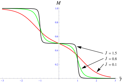
Figure 2: The curved state density $M=\frac{1}{N}\sum\nolimits_{i=1}^{N}\left\langle\sigma_{i}^{k}\right\rangle$ versus the state bias parameter $\widetilde{\gamma}$ for different values of coupling constant$\ \widetilde{J}$ and fixed stiffness $\widetilde{B}=1.$ Note the broad $\widetilde{\gamma}$ independent plateau region for $\widetilde{J}=1.5$ where $M=1/2.$ For large values of $\left|\widetilde{\gamma}\right|,$ $M$ is either $0$ or $1$ corresponding to straight unstrained or straight strained lattice states respectively.

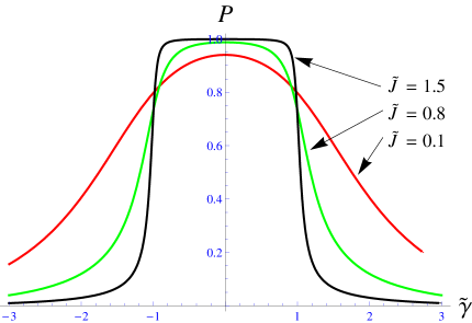
Figure 3: Plot of the mean polymorphic polarization $P$ of the reduced two block model versus the conformational bias field $\widetilde{\gamma}$ for different values of coupling constant $\widetilde{J}$ and effective tube stiffness $\widetilde{B}=1.$ For $\widetilde{J}\geq 1.5,$ the tube’s curvature is at maximum for $\left|\widetilde{\gamma}\right|<1,$ as $P\approx 1$ in this region. For larger $\left|\widetilde{\gamma}\right|,$ the tube is in a straight state and $P$ goes to zero.

III.1 Simple case $\widetilde{\gamma}=0$

In this case all quantities can be computed in compact form. In particular the largest eigenvalue of the transfer matrix simplifies to $\lambda_{1}=2\cosh(\widetilde{B})\cosh(2\widetilde{J})+D$ with $D=(3+\cosh(2\widetilde{B})+2\cosh(4\widetilde{J})\sinh^{2}(\widetilde{B}))^{1/2}.$ As already mentioned the curved state density is constant $M=1/2$ (independent of $\widetilde{B}$ and $\widetilde{J}$), whereas the total ”polarization” is $P^{2}=1-2\left\langle\sigma_{i}^{1}\sigma_{i}^{2}\right\rangle=\frac{1}{2}+\frac{\sinh(\widetilde{B})\cosh(2\widetilde{J})}{D}$ which tends to $1$ for $\widetilde{J}\gtrsim 1$. This means that $\left\langle\sigma_{i}^{1}\sigma_{i}^{2}\right\rangle\rightarrow 0$ which can be understood as both states (on opposing ladder sides) at the same site $i$ fluctuate alternately between $0$ and $1.$ The coupling $\widetilde{J}$ which is a measure of the cooperativity determines over which distance the curved state is coherent. The cooperativity can be measured by the spin-spin correlation function $g_{ij}^{kl}=\left\langle\sigma_{i}^{k}\sigma_{j}^{l}\right\rangle-\left\langle\sigma_{i}^{k}\right\rangle\left\langle\sigma_{j}^{l}\right\rangle=\left\langle\sigma_{i}^{k}\sigma_{j}^{l}\right\rangle-1/4$ with $k,l=1,2$ at two different sites $i$ and $j$. By symmetry $g_{ij}^{11}=g_{ij}^{22}$ and $g_{ij}^{12}=g_{ij}^{21}.$ Introducing the two matrices $\underline{V}^{1}$ and $\underline{V}^{2}$ defined as

$$\underline{V}^{1}=\left(\begin{array}[c]{cccc}1&0&0&0\\ 0&1&0&0\\ 0&0&-1&0\\ 0&0&0&-1\end{array}\right)\text{ \ and }\underline{V}^{2}=\left(\begin{array}[c]{cccc}1&0&0&0\\ 0&-1&0&0\\ 0&0&1&0\\ 0&0&0&-1\end{array}\right)$$

the correlation functions of the variable $S^{k}$ with $k=1,2$ can be written as $\left\langle S_{i}^{k}S_{j}^{l}\right\rangle=\frac{1}{Z}$Tr$(T^{i-1}\underline{V}^{k}T^{j-i-1}\underline{V}^{l}T^{N-j+i+1})$ for $i<j.$ With the matrix $U$ diagonalizing $T$, i.e. $U^{-1}TU=\Lambda$ and the following transformed matrices $V^{k}=U^{-1}\underline{V}^{k}U$, we have $\left\langle S_{i}^{k}S_{j}^{l}\right\rangle=\frac{1}{Z}$Tr$(\Lambda^{i-1}V^{k}\Lambda^{j-i}V^{l}\Lambda^{N-j+1}).$ In the limit $N\rightarrow\infty,$ this expression can be evaluated :

$$\left\langle S_{i}^{k}S_{j}^{l}\right\rangle =V_{11}^{k}V_{11}^{l}+\left(\frac{\lambda_{2}}{\lambda_{1}}\right)^{j-i}V_{21}^{k}V_{12}^{l}$$

$$+\left(\frac{\lambda_{3}}{\lambda_{1}}\right)^{j-i}V_{31}^{k}V_{13}^{l}+\left(\frac{\lambda_{4}}{\lambda_{1}}\right)^{j-i}V_{41}^{k}V_{41}^{l}$$ (8)

where the eigenvalues are ordered $\lambda_{1}>..>\lambda_{4}.$ From Eq. 8 all $g_{ij}^{kl}$ can be deduced. It turns out that the most interesting quantity connected to the spatial fluctuations of the microtubule -its persistence length (see next section) - is connected to $\Delta g_{ij}\equiv g_{ij}^{11}-g_{ij}^{12}=\left\langle\sigma_{i}^{1}\sigma_{j}^{1}\right\rangle-\left\langle\sigma_{i}^{1}\sigma_{j}^{2}\right\rangle.$ An explicit computation of the matrix elements of $V^{k}$ shows that $V_{14}^{k}=V_{11}^{k}=0$ and $V_{31}^{1}V_{13}^{1}=V_{13}^{2}V_{31}^{1}$ as well as $V_{21}^{1}V_{12}^{1}=-V_{12}^{2}V_{21}^{1}=P^{2}$. This leads to

$$\Delta g_{ij}=\frac{1}{2}P^{2}\exp(-\left|i-j\right|/\widetilde{\xi})$$ (9)

where the correlation length is $\widetilde{\xi}=\left[\ln\left(\frac{\lambda_{1}}{\lambda_{2}}\right)\right]^{-1}$ with $\lambda_{2}=2\exp(\widetilde{B})\sinh(2\widetilde{J}).$ With the result for $2$ blocks (ladder model, Fig 1E) we are now able to compute the persistence length for the $4$-block polymorphic tube (Fig 1B).

IV Angular persistence length

The persistence length $l_{p}$ is the length scale characterizing the filament’s resistance to thermally induced bending moments. For usual biofilaments like DNA or actin filaments $l_{p}=l_{B}$ is a material constant equal to the bending persistence length $l_{B}\equiv B/k_{B}T$. However for microtubules $l_{p}$ is known to be length dependent Pampaloni . Here we compute the angular persistence length for the $4$-block model from the usual definition in terms of the tangent-tangent correlation function $\left\langle\overrightarrow{t}(s^{\prime})\cdot\overrightarrow{t}(s)\right\rangle=\exp(-\left|s^{\prime}-s\right|/l_{p})$ where $\overrightarrow{t}(s)$ is the unit-tangent vector at the position $s$ of the microtubule centerline. From $\overrightarrow{t}(s)=(\theta_{x}(s),\theta_{y}(s),\sqrt{1-\theta_{x}^{2}(s)-\theta_{y}^{2}(s)})$ in the external frame, we deduce to quadratic order in $\theta$ that $\left\langle\overrightarrow{t}(s^{\prime})\cdot\overrightarrow{t}(s)\right\rangle\approx 1-\frac{1}{2}V(s^{\prime}-s)$ with the angular variance $V(s^{\prime}-s)=\left\langle(\theta_{x}(s^{\prime})-\theta_{x}(s))^{2}\right\rangle+\left\langle(\theta_{y}(s^{\prime})-\theta_{y}(s))^{2}\right\rangle.$ Therefore one can write $\left\langle\overrightarrow{t}(s^{\prime})\cdot\overrightarrow{t}(s)\right\rangle\approx\exp(-\left|s^{\prime}-s\right|/l_{p})$ with a persistence length $l_{p}(s^{\prime}-s)=2\frac{\left|s^{\prime}-s\right|}{V(s^{\prime}-s)}$ that will be manifestly distance dependent in our case. Now by writing $\overrightarrow{\theta}=\overrightarrow{\theta}_{pol}+\overrightarrow{\theta}_{el}$ and from the independence of polymorphic and elastic contributions $\left\langle\overrightarrow{\theta}_{pol}\cdot\overrightarrow{\theta}_{el}\right\rangle=\left\langle\overrightarrow{\theta}_{pol}\right\rangle\cdot\left\langle\overrightarrow{\theta}_{el}\right\rangle=0,$ we deduce that the total persistence length can be decomposed as $l_{p}=(\frac{1}{l_{B}}+\frac{1}{l_{pol}})^{-1}$ with a polymorphic persistence length

$$l_{pol}(s^{\prime}-s)=2\frac{\left|s^{\prime}-s\right|}{V_{pol}(s^{\prime}-s)}$$ (10)

At this level, for the geometric description of the microtubule shape in space it is more convenient to use a continuum description and replace the discrete index $i$ by the continuous variable $s,$ so that $\overrightarrow{\theta}_{pol,i}\rightarrow\overrightarrow{\theta}_{pol}(s)$ which is obtained from the integration over $s$ of the curvature Eq. 5

$$\overrightarrow{\theta}_{pol}(s)=\overrightarrow{\theta}_{pol}(0)+\int_{0}^{s}\vec{\kappa}_{pol}(s)ds$$ (11)

Now we can compute the polymorphic variance from the correlation function $G_{pol,x}(s^{\prime},s)=\left\langle(\theta_{pol,x}(s^{\prime})-\theta_{x}(0)(\theta_{pol,x}(s)-\theta_{x}(0))\right\rangle.$ Note that by symmetry $G_{pol,y}(s^{\prime},s)=G_{pol,x}(s^{\prime},s).$ From Eqs. 11,9 we readily obtain for the full $4$-block model

$$G_{pol,x}(s^{\prime},s) =\frac{\kappa_{1}^{2}P^{2}}{2}\int_{0}^{s^{\prime}}\int_{0}^{s}ds_{1}ds_{2}\cos\left(q_{0}(s_{2}-s_{1}\right))$$

$$\exp\left(-\frac{\left|s_{2}-s_{1}\right|}{\widetilde{\xi}b}\right).$$ (12)

where for a free microtubule (not angularly constrained at the ends) we have to integrate over the arbitrary initial angle $\varphi\in\left[0,2\pi\right].$ The variance can now be computed and we obtain :

$$V_{pol}(s^{\prime}-s) =\frac{2\kappa_{1}^{2}P^{2}\xi}{1+\xi^{2}q_{0}^{2}}\left\{\left|s^{\prime}-s\right|-\frac{1-\xi^{2}q_{0}^{2}}{1+\xi^{2}q_{0}^{2}}\xi\right.$$

$$+\frac{\xi e^{-\left|s^{\prime}-s\right|/\xi}}{1+\xi^{2}q_{0}^{2}}\left(\left(1-q_{0}^{2}\xi^{2}\right)\cos\left(q_{0}(s^{\prime}-s)\right)\right.$$

$$\left.\left.-2q_{0}\xi\sin\left(q_{0}\left|s^{\prime}-s\right|\right)\right)\right\}$$ (13)

with $\xi=\widetilde{\xi}b.$ From Eq. 13 the persistence length $l_{pol}$ and thus $l_{p}$ can be deduced. The polymorphic variance Eq. 13 has the following generic asymptotic behaviors : At large distance $s>>\xi,$ the variance $V_{pol}(s)\approx 2\kappa_{1}^{2}P^{2}\frac{\xi}{1+\xi^{2}q_{0}^{2}}s$ scales linearly with $s$ indicating that $\overrightarrow{\theta}_{pol}$ is performing a simple (angular) random walk. At such a scale the microtubule looses its ”coherent nature” and is replaced by a collection of uncorrelated segments. So not surprisingly we recover the classical results of a semiflexible chain again. In this asymptotic regime the effective persistence length reaches saturation with a renormalized constant value $l_{p}\left(\infty\right)=1/\left(l_{pol}^{-1}+l_{B}^{-1}\right)$ where

$$l_{pol}\left(\infty\right)=\frac{1+\xi^{2}q_{0}^{2}}{\xi\kappa_{1}^{2}P^{2}}$$ (14)

At short distance such that $s<<$min($\xi,q_{0}^{-1}$) the variance has a quadratic behavior $V_{pol}(s)\approx\kappa_{1}^{2}P^{2}s^{2}$. In this regime, the polymorphic fluctuations are completely dominated by purely ”classical” semiflexible chain fluctuations and $l_{p}\left(0\right)=l_{B}.$ Starting from this value of $l_{p}$ at $s=0$, polymorphic fluctuations begin to contribute reducing the persistence length $l_{p}\left(s\right)\approx(\frac{1}{l_{B}}+\frac{\kappa_{1}^{2}P^{2}s}{2})^{-1}$. This behavior is universal and independent of $\xi$ and $q_{0}^{-1}.$

In the intermediate regime with $s$ of the order of $\xi$, the behavior of $V_{pol}(s)$ depends on the value of $\xi q_{0}$ - a kind of ”helix coherence” parameter. When $\xi q_{0}\leq 1$ (low helix coherence) oscillations in Eq. 13 are damped and the persistence length $l_{p}\left(s\right)$ is monotonously deceasing from $l_{B}$ to the constant $l_{p}\left(\infty\right)$ with $l_{pol}\left(\infty\right)\approx(\xi\kappa_{1}^{2}P^{2})^{-1}$ obtained from Eq. 14 (cf. Fig.4). This corresponds also to the situation of no internal twist $q_{0}=0.$

In the most interesting (high helical coherence) regime $\xi q_{0}>1,$ the behavior of $V_{pol}(s)$ is a combination of two effects: an oscillation with wave length $\lambda=2\pi q_{0}^{-1}$ originating from the helical nature of the microtubule, but which is now damped by the presence of thermally induced defects (due to a finite $\xi$) reducing the coherence of the helix and enhancing the linearly growing behavior (the random walk). As a consequence for high helical coherence $l_{p}\left(s\right)$ displays three different regimes (cf Fig.4):

I. In the limit of very short , $l_{p}\left(s\right)\approx(\frac{1}{l_{B}}+\frac{\kappa_{1}^{2}P^{2}s}{2})^{-1}$ that attains a global minimum at $s_{\min}\approx\pi q_{0}^{-1}$

II. For intermediate length values $s_{\min}<s\lesssim$ $\xi$, the total persistence length displays a non-monotonic oscillatory behavior of period $\lambda$ with damped amplitude around a nearly linearly growing average reflecting the polymorphic fluctuation of the helix.

III. For distances $s>>\xi,$ the oscillations in Eq. 13 are completely damped as the helix forgets its ”coherent nature” on these scales and reaches the limiting value $l_{p}^{\ast}\left(\infty\right)=1/\left(l_{pol}^{-1}+l_{B}^{-1}\right)$ with $l_{pol}\left(\infty\right)$ given by Eq. 14.

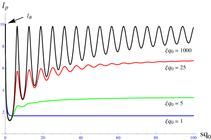
Figure 4: Representative plots of the angular persistence length $l_{p}$ versus distance along contour $s$ for intrinsic elastic bending stiffnes $l_{B}=10\mu m$ (chosen arbitrary and small for pictorial convenience) and different values of scaled correlation length $\xi q_{0}.$

V High cooperativity limit and uniform states

In the previous paragraphs we considered the thermodynamic limit $L=Nb\rightarrow\infty$ for which the correlation length $\xi$ is always smaller that the total length $L$ Footnote1 . It also interesting to consider the opposite regime $\xi>>L$. In this case of large cooperativity we may take formally the limit $J\rightarrow\infty$ . Consequently the two states variables $\sigma^{i}$ become uniform all along their respective block axes $i=1..4$. The decoupling of the full MT lattice into 2 independent $2\times 2$ sub-blocks implies the equality of the energy and entropy of the two independent 2-sub-blocks sets so that we can focus on only a single sub-lattice made of two blocks, say $1$ and $2.$ The corresponding polymorphic energy is $E=\frac{B\kappa_{1}^{2}}{2}L\left[(\frac{\pi}{2}\gamma-1)\left(\sigma^{1}+\sigma^{2}\right)+2\sigma^{1}\sigma^{2}\right]$ and its partition function reads now $Z=1+2\exp\left(-2(\widetilde{\gamma}-\widetilde{B})L/b\right)+\exp\left(-4\widetilde{\gamma}L/b\right).$ For two blocks there are then only 4 possible states with different probabilities of realization $\rho(\sigma^{1},\sigma^{2})=\exp(-\beta E)/Z$ that are: $\rho(0,0)=1/Z$ for the straight unstrained state, $\rho(1,1)=\exp\left(-4\widetilde{\gamma}L/b\right)/Z$ for the straight prestrained state and finally $\rho(0,1)=\rho(1,0)=\exp\left(-2(\widetilde{\gamma}-\widetilde{B})L/b\right)/Z$ for the two polymorphic helical states. The average value of the spin and the correlation functions are given respectively by $\left\langle\sigma^{k}\right\rangle=\rho(1,0)+\rho(1,1)$ for $k=1..4$ and $\left\langle\sigma^{1}\sigma^{2}\right\rangle=\left\langle\sigma^{3}\sigma^{4}\right\rangle=\rho(1,1)$.

Going back to the full lattice model made of four blocks the polymorphic order parameter is then given $P^{2}(L)=2(\left\langle\sigma^{1}\right\rangle-\left\langle\sigma^{1}\sigma^{2}\right\rangle+\left\langle\sigma^{3}\right\rangle-\left\langle\sigma^{3}\sigma^{4}\right\rangle)=4\rho(1,0)$. The angular variance at position $s$ and $s^{\prime}$ can be easily computed and we find $V(s^{\prime}-s)=\frac{\kappa_{1}^{2}P^{2}(L)}{q_{0}^{2}}\left(1-\cos\left(q_{0}(s^{\prime}-s\right))\right)$ which obviously corresponds to the limit of infinite $\xi$ of Eq. 13 but with the additional factor $P^{2}(L)$ responsible for the length dependence of the variance. The weight of the different possible configurations depends on $\widetilde{\gamma}$ and the discrimination between them is more pronounced with growing length. This can be easily understood from the polymorphic entropy $\Sigma_{\sigma}$ which remarkably is non extensive. Note that $\Sigma_{\sigma}$ is always twice the entropy of the individual 2-block-sub-lattices. For the asymptotic limiting case of short $L\rightarrow 0$ all $4\times 4$ configurations of the full lattice have the same probability and therefore $\Sigma_{\sigma}(0)=2k_{B}\ln 4.$ For larger $L,$ the entropy will continuously change to reach a constant value depending on the dominant configurations that are selected by $\gamma.$ For values of $\left|\widetilde{\gamma}\right|>\widetilde{B}$, we see on Fig. 5 that $P(L)$ goes to zero with growing values of $L$. In this regime there is only one configuration (the same for the two sublattices) $\rho(0,0)$ or $\rho(1,1)$ depending on the sign of $\widetilde{\gamma}$ and $\Sigma_{\sigma}(L)\rightarrow 0.$ Interestingly for $\widetilde{\gamma}=\pm\widetilde{B},$ there is an additional configuration for a given sub-lattice with the same probability $\rho(0,1)=\rho(1,1)=\rho(0,0)=1/Z,$ so that for the 4-blocks we have $3\times 3$ configurations and $\Sigma_{\sigma}(L)\rightarrow 2k_{B}\ln 3.$ This coexistence leads to a state which is the superposition between straight and curved states with different probability such that $P^{2}(L)=\frac{4}{3+\exp\left(-4\widetilde{B}L/b\right)}\approx\frac{4}{3}$ that is (quasi) length independent. When $\left|\widetilde{\gamma}\right|$ is very close to $\widetilde{B}$ , the evolution of $\Sigma_{\sigma}(L)$ versus $L,$ can be slow and therefore there is a regime of lengths where the the entropy is non-extensive and where the straight states have comparable free energy with the helical one. In this regime the microtubule will fluctuate between its almost degenerate straight and (two) curved states.

For $\left|\widetilde{\gamma}\right|<\widetilde{B},$ there are for a given sub-lattice two dominant degenerate configurations $(0,1)$ and $(1,0),$ so that the number of configuration for the full lattice model is $2\times 2$ and $\Sigma_{\sigma}(L)\rightarrow 2k_{B}\ln 2$ with growing $L.$ In this regime the mean curvature is built up progressively with the length $L,$ to reach -faster for smaller value of $\left|\widetilde{\gamma}\right|$ - its maximum value $P=\sqrt{2}.$ Here also when $\left|\widetilde{\gamma}\right|$ is very close to $\widetilde{B}$ the realization of the curved state can be slow with growing $L.$

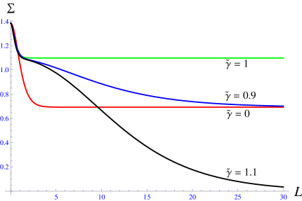
Figure 5: Polymorphic entropies $\Sigma$ (four-block model) versus the microtubule’s length $L$ for different values of conformational bias $\widetilde{\gamma}$ and stiffness $\widetilde{B}=1.$

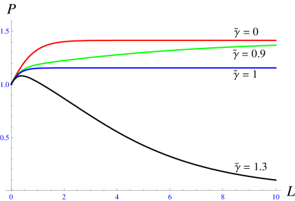
Figure 6: Plots of the polymorphic polarization $P$ (four-block model) versus the microtubule’s length $L$ for different values of $\widetilde{\gamma}$ and with $\widetilde{B}=1.$ We observe that microtubule curvature can be build up progressively with growing MTs.

VI Angular power spectrum

Other information on the equilibrium properties of the microtubule can be deduced from the analysis of its Fourier mode distribution. To do so we express the microtubule shape $\overrightarrow{\theta}(s)$ as a superposition of Fourier modes $\overrightarrow{\theta}(s)=\overrightarrow{\theta}(0)+\sqrt{2/L}\sum_{n=1}^{+\infty}\overrightarrow{a}_{n}\cos(q_{n}s)+\sqrt{2/L}\sum_{n=1}^{+\infty}\overrightarrow{b}_{n}\sin(q_{n}s)+\left(\theta_{x}(L)-\theta_{x}(0)\right)s/L$ with the wave vector $q_{n}=\frac{2n\pi}{L}$ and where we add the ”ramp term” $\left(\theta_{x}(L)-\theta_{x}(0)\right)s/L,$ as $\overrightarrow{\theta}(s)$ is not a periodic function in general, i.e., $\overrightarrow{\theta}(L)\neq\overrightarrow{\theta}(0)$ Footnote2 . Decomposing the shape as $\overrightarrow{\theta}(s)=\overrightarrow{\theta}_{pol}(s)+\overrightarrow{\theta}_{el}(s)$ we readily see that the equilibrium square of the amplitude of the elastic Fourier modes $G_{el}(q_{n})\equiv\left\langle\overrightarrow{a}_{el,n}^{2}\right\rangle=\left\langle\overrightarrow{b}_{el,n}^{2}\right\rangle=\frac{2}{l_{B}q_{n}^{2}}$ has the usual thermally driven elastic bending spectrum of a wormlike chain. On the other hand from Eq. 12 the polymorphic mode distribution $G_{pol}(q)$ in the limit $L$ large (with $q_{n}\rightarrow q$ continuous) can be deduced :

$$G_{pol}(q)=\frac{2\kappa_{1}^{2}P^{2}\xi}{q^{2}}\cdot\frac{1+\xi^{2}(q^{2}+q_{0}^{2})}{1+\xi^{4}(q^{2}-q_{0}^{2})^{2}+2\xi^{2}(q^{2}+q_{0}^{2})}$$ (15)

As shown in Fig. 6, when the correlation length $\xi$ is of order of the helix pitch $\lambda=2\pi/q_{0}$, the function $G_{pol}(q)$ departs very much from the wormlike chain bending spectrum $G_{el}(q)$ and displays a non-monotonous shape with a peak at $q_{0}$. This peak is more pronounced and sharper for larger value of $\xi q_{0}$ (helix more coherent) and disappears when $\xi q_{0}\leq 1$. This is the main Fourier mode signature of the -polymorphic fluctuating- helicoidal nature of the microtubule. For long wavelength modes $q<<q_{0},$ the spectrum has a semiflexible like behavior $G_{pol}(p)\approx\frac{2}{l_{pol}\left(\infty\right)q^{2}}$ reflecting the incoherence of the helix at this scale, with the persistence length given by Eq. 14. For short wavelength modes $q>>q_{0},$ the behavior becomes quarticaly decreasing $G_{pol}(p)\approx\frac{2\kappa_{1}^{2}}{\xi q^{4}}$ and polymorphic fluctuations are strongly damped at short distance in agreement with high cooperativity at this scale.

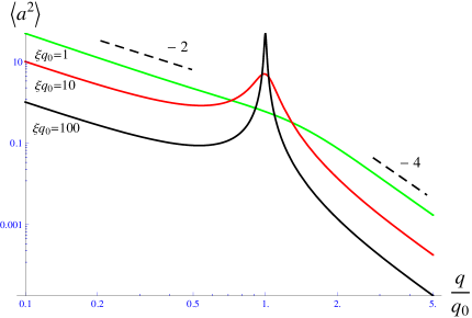
Figure 7: Log-Log plot of the polymorphic Fourier mode distribution $G_{pol}(q)$ for different values of $\xi q_{0}.$ Besides a characteristic peak at $q_{0}$ one observes a cross-over between a small $q$ regime with scaling $q^{-2}$ and a large $q$ regime with a $q^{-4}$ scaling.

Quantitative comparison with experiments at this point seems difficult, because Fourier analysis of microtubules in-vitro was mainly performed on microtubules strongly confined into an almost 2-D geometry. This experimental necessity (originating from optical microscopy sample flatness requirements) is expected to induce artifacts as in this case, within our helical model, the microtubules would likely not fully equilibrate between their different equivalent curved states as large barriers will appear under confinement. In agreement with this argument the experimental Fourier modes of microtubules systematically reveal some type of ”frozen-in” curvature which is much larger than the fluctuations around it GITTES - in particular for longer wavelength modes. This is in so far striking as no clear argument for large systematic built-in curvature in microtubules (other than the here described) is evident, indicating that this curvature is in fact the very character of the microtubule elasticity. Similarly in vivo, it was found that growing microtubules have large scale frozen-in curvature Brangwyne . This phenomenon was interpreted in terms of a random interaction of the growing microtubule tip with the surrounding cytoskeleton. Instead it could be that the curvature has an intrinsic origin (like in the present model) but is not allowed to fully equilibrate due to constraints present in the cytoplasm.

VII Conclusion and Outlook

We have investigated the thermodynamics of a toy model for cooperatively switching (polymorphic) biofilaments, whose paradigm example is believed to be the microtubule. The polymorphism of the microtubule’s subunits and the short range cooperative interaction leads to properties that are very different from usual biofilaments. In particular the ground state itself is not a single fixed shape but is found to consist of a set of degenerate helicoidal configurations. At finite temperature, the fluctuations of the subunits create defects that smoothen the perfect helix and can even destroy it on very long scale where the filament retrieves a typical worm-like chain behavior. Another peculiar characteristic of the polymorphic tube is the length dependence of the persistence length. The Fourier spectrum turns out also to be markedly different from classical biofilaments. While it has a typical semiflexible chain behavior at long scale the Fourier modes amplitude are enhanced for modes around the characteristic scale of the helix. At very short scales the modes are strongly dampened due to the strong cooperative dimer interaction. We believe that the Fourier spectrum will be of some value to discriminate between different models in the analysis of future experiments (as in Pampaloni ) where confinement is absent and microtubules can thus rearrange and equilibrate.

The model developed here was inspired and tailored to microtubules. However it can be adapted to other polymorphic filaments with similar cross-sectional symmetry (circular rod or tube). Polymorphic sheets, rods and tubes are not uncommon in nature with the best documented example the bacterial flagellum Flagellum . In the latter case the polymorphic states are likely very rigid (or coherent in our terminology) on thermal energy scales with correlation lengths $\xi$ larger than filament’s length $L$. Rearrangements between equivalent lattice states could then face high barriers in the flagellum and suppress the here described polymorphic fluctuations on measurement time scales. However other filaments might be even better candidates for soft polymorphic tubes (or rods) and deserve a closer investigation. Observations of unusual flaring-up of peculiar helical modes in bacterial pili (cf. Fig. 1 in Pili ) as well as in actin filaments cooperatively interacting with drugs like cofilin (cf. Fig. 1c in ActinCofilin ) visually suggest the presence of soft polymorphic mode dynamics.

References

- (1) Alberts, B., A. Johnson, J. Lewis, M. Raff, K. Roberts, and P. Walter. 2005. Molecular Biology of the Cell.
- (2) Mohrbach, H., A. Johner, and I. M. Kulic. 2010. Tubulin bistability and polymorphic dynamics of microtubules. Phys. Rev. Lett. 105:268102; Cooperative Lattice Dynamics and Anomalous Fluctuations of Microtubules. arXiv:1108.4800 cond-mat.soft. 2011, Submitted.
- (3) Taute, K. M., F. Pampaloni2, E. Frey, and E-L. Florin, 2008. Microtubule dynamics depart from the wormlike chain model. Phys. Rev. Lett. 100, 028102.
- (4) Pampaloni, F., G. Lattanzi, A. Jonas, T. Surrey, E. Frey, and E. L. Florin. 2006. Thermal fluctuations of grafted microtubules provide evidence of a length-dependent persistence length. Proc. Natl. Acad. USA. 103:10248-10253.
- (5) Venier, P., A. C. Maggs, M. F. Carlier, and D. Pantaloni. 1994. Analysis of microtubule rigidity using hydrodynamic flow and thermal fluctuations. J. Biol. Chem. 269: 13353.
- (6) Wade, R. H., D. Chrétien, and D. Job. 1990. Characterization of microtubule protofilament numbers. How does the surface lattice accommodate?. J. Mol. Bio. 212:775-786.
- (7) Chretien, D., and R. H. Wade. 1991. New data on the microtubule surface lattice. Bio. Cell. 71:161-174.
- (8) Bouchet-Marquis, C., B. Zuber, A-M. Glynn, M. Eltsov, M. Grabenbauer, K. N. Goldie, D. Thomas, A. S. Frangakis, J. Dubochet, and D. Chrétien. 2007. Visualization of cell microtubules in their native state. Bio. Cell. 99:45-53.
- (9) Ray, S., E. Meyhofer, R. A. Milligan, and J. Howard. 1993. Kinesin follows the microtubule’s protofilament axis. J. Cell Biol. 121:1083-1093.
- (10) Chretien, D., and S. D. Fuller. 2000. Microtubules switch occasionally into unfavorable configurations during elongation. J. Mol. Biol. 298:663-676.
- (11) The periodic boundary conditions on the spin inherent to the tranfer matrix method implies that Eq. 9 is valid for For of order we need to consider free boundary conditions for which we have computed the spin correlations numerically for growing values of A difference between numerics and the analytical - asymptotic expression Eq. 9 comes from the correlation function that decreases suddently slightly faster than for or near the ends. This boundary effect is rapidly negligeable and already for a very good correspondance between the numerics and 9 was found.
- (12) We have tried the more conventional decomposition as in GITTES and, from it, computed the variance and found that is does not give Eq. 13. Fourier decomposition around a non-trivial ground state is a complex issue with mathematical ”underwater mines” that we will discuss elsewhere.
- (13) Gittes, F., B. Mickey, J. Nettleton, and J. Howard. 1993. Flexural rigidity of microtubules and actin filaments measured from thermal fluctuations in shape. J. Cell Biol. 120:923-934; Brangwynne, C., G. Koenderink, E. Barry, Z. Dogic, F. MacKintosh, and D. Weitz. 2007. Bending dynamics of fluctuating biopolymers probed by automated high-resolution filament tracking. Biophys. J. 93:346-359; Janson, M. E. and M. Dogterom. 2004. A bending mode analysis for growing microtubules: evidence for a velocity-dependent rigidity. Biophys. J. 87:2723-2736.
- (14) Brangwyne C., F. C. MacKintosh, D. A. Weitz. 2007. Force Fluctuations and Polymerization Dynamics of Intracellular Microtubules. PNAS. 104:16128-16133.
- (15) S. V. Srigiriraju & T. R. Powers Phys. Rev. Lett. 94, 248101 (2005); H. Wada and R. R. Netz, Europhys. Lett, 82, 28001 (2008)
- (16) J.M. Skerker and H.C.Berg, Direct observation of extension and retraction of type IV pili. PNAS 98, 126901 (2001)
- (17) B.R. McCullough, L.B., J-L M. , E. M. De La Cruz , Cofilin Increases the Bending Flexibility of Actin Filaments: Implications for Severing and Cell Mechanics, J. Mol. Biol. (2008) 381, 550– 558