Dark energy model with variable $q$ and $\omega$ in LRS Bianchi-II space-time

Abstract

The present study deals with spatial homogeneous and anisotropic locally rotationally symmetric (LRS) Bianchi-II dark energy model in general relativity. The Einstein’s field equations have been solved exactly by taking into account the proportionality relation between one of the components of shear scalar $(\sigma^{1}_{1})$ and expansion scalar $(\vartheta)$, which, for some suitable choices of problem parameters, yields time dependent equation of state (EoS) and deceleration parameter (DP), representing a model which generates a transition of universe from early decelerating phase to present accelerating phase. The physical and geometrical behavior of universe have been discussed in detail.

Key words: Dark energy, variable DP and EoS parameter.

PACS Nos: 98.80Es, 98.80-k, 95.36.+x

1 Introduction

The discovery of acceleration of the universe stands as a major breakthrough of the observational cosmology. The power of observations in cosmology is clear from the observations of supernovae of Ia (SN Ia) which dramatically changed, about a decade ago, the then standard picture of cosmology - of an expanding universe evolving under the rules of general relativity such that the expansion rate should slow down as cosmic time unfolds. Surveys of cosmologically distant SN Ia (Riess et al. 1998; Permutter et al. 1999) indicated the presence of new, unaccounted - for $\it{dark\;energy}$ that opposes the self-attraction of matter and causes the expansion of the universe to accelerate. When combined with indirect measurements using cosmic microwave background (CMB) anisotropies, cosmic shear and studies of galaxy clusters, a cosmological world model has emerged that describes the universe at flat, with about $70\%$ of it’s energy contained in the form of this cosmic dark energy (Seljak et al. 2005). This acceleration is realized with negative pressure and positive energy density that violate the strong energy condition. This violation gives a reverse gravitational effect. Due to this effect, the universe gets a jerk and the transition from the earlier deceleration phase to the recent acceleration phase take place (Caldwell et al 2002). The cause of this sudden transition and the source of accelerated expansion is still unknown. In physical cosmology and astronomy, the simplest candidate for the DE is the cosmological constant $(\Lambda)$, but it needs to be extremely fine-tuned to satisfy the current value of the DE density, which is a serious problem. Alternatively, to explain the decay of the density, the different forms of dynamically changing DE with an effective equation of state (EoS), $\omega=p/\rho<-1/3$, were proposed instead of the constant vacuum energy density. Other possible forms of DE include quintessence $(\omega>-1)$ (Steinhardt et al. 1999), phantom $(\omega<-1)$ (Caldwell 2002) etc. While the the possibility $\omega<<-1$ is ruled out by current cosmological data from SN Ia (Supernovae Legacy Survey, Gold sample of Hubble Space Telescope) (Riess et al. 2006; Astier et al. 2006), CMBR (WMAP, BOOMERANG) (Eisentein et al. 2005; MacTavish et al. 2006) and large scale structure (Sloan Digital Sky Survey) data (Komatsu et al. 2009), the dynamically evolving DE crossing the phantom divide line (PDL) $(\omega=-1)$ is mildly favored. Some other limits obtained from observational results coming from SNe Ia data (Knop et al 2003) and combination of SNe Ia data with CMBR anisotropy and galaxy clustering statistics (Tegmark et al. 2004) are $-1.67<\omega<-0.62$ and $-1.33<\omega<-0.79$, respectively. The latest results in 2009, obtained after a combination of cosmological data-sets coming from CMB anisotropies, luminosity distances of high red-shift type Ia supernovae and galaxy clustering, constrain the dark energy EoS to $-1.44<\omega<-0.92$ at $68\%$ confidence level (Komatsu et al. 2009; Hinshaw et al. 2009)

Moreover, in recent years Bianchi universes have been gaining an increasing interest of observational cosmology, since the WMAP data (Hinshaw et al. 2003, 2007; Jaffe et al. 2005) seem to require an addition to the standard cosmological model with positive cosmological constant that resembles the Bianchi morphology (Jaffe et al. 2006a, 2006b; Campanelli et al. 2006, 2007; Hoftuft et al. 2009). According to this, the universe should achieve a slightly anisotropic special geometry in spite of the inflation, contrary to generic inflationary models and that might be indicating a nontrivial isotropization history of universe due to the presence of an anisotropic energy source. The Bianchi models isotropize at late times even for ordinary matter, and the possible anisotropy of the Bianchi metrics necessarily dies away during the inflationary era (Ellis 2006). In fact this isotropization of the Bianchi metrics is due to the implicit assumption that the DE is isotropic in nature. Therefore, the CMB anisotropy can also be fine tuned, since the Bianchi universe anisotropies determine the CMB anisotropies. The price of this property of DE is a voilation of null energy condition (NEC) since the DE crosses the phantom divide line (PDL), in particular depending on the direction.

The anomalies found in the cosmic microwave background (CMB) and large scale structure observations stimulated a growing interest in anisotropic cosmological model of universe. Here we confine ourselves to models of Bianchi-type II. Bianchi type-II space-time has a fundamental role in constructing cosmological models suitable for describing the early stages of evolution of universe. Asseo and Sol (1987) emphasized the importance of Bianchi type-II Universe. Recently Pradhan et al (2011) and Kumar and Akarsu (2011) have dealt with Bianchi-II DE models by considering the spatial law of variation of Hubble’s parameter which yields the constant value of deceleration parameter (DP). Some authors (Akarsu and Kilinc 2010a, 2010b; Yadav et al. 2011; Yadav and Yadav 2011; Kumar and Yadav 2011; Yadav 2011; Adhav et al. 2011 and recently Yadav and Saha 2011) have studied DE models with variable EoS parameter. In this paper, we presented general relativistic cosmological model with time dependent DP in LRS Bianchi-II space-time which can be described by isotropic and variable EoS parameter. The paper is organized as follows: The metric and field equation are presented in section 2. Section 3 deals with the solution of field equations and physical behavior of the model. Finally the findings of paper are discussed in section 4.

2 The metric and field equations

The gravitational field in our case is given by a Bianchi type-II (BII) metric

$$ds^{2}=-dt^{2}+a_{1}^{2}(dx_{1}-x_{3}dx_{2})^{2}+a_{2}^{2}dx_{2}^{2}+a_{3}^{2}dx_{3}^{2},$$ (1)

with $a_{1},\,a_{2},\,a_{3}$ being the functions of time only. In what follows, we consider the LRS BII model setting $a_{2}=a_{3}$.

Given the fact that the dark energy is isotropically distributed, it is enough to consider only three Einstein equations (Saha 2011) corresponding to the metric (1), namely

$$2\frac{\ddot{a}_{2}}{a_{2}}+\Bigl{(}\frac{\dot{a}_{2}}{a_{2}}\Bigr{)}^{2}-\frac{3}{4}\frac{a_{1}^{2}}{a_{2}^{4}} = -\omega\rho,$$ (2a)

$$\frac{\ddot{a}_{1}}{a_{1}}+\frac{\ddot{a}_{2}}{a_{2}}+\frac{\dot{a}_{1}}{a_{1}}\frac{\dot{a}_{2}}{a_{2}}+\frac{1}{4}\frac{a_{1}^{2}}{a_{2}^{4}} = -\omega\rho,$$ (2b)

$$2\frac{\dot{a}_{1}}{a_{1}}\frac{\dot{a}_{2}}{a_{2}}+\Bigl{(}\frac{\dot{a}_{2}}{a_{2}}\Bigr{)}^{2}-\frac{1}{4}\frac{a_{1}^{2}}{a_{2}^{4}} = \rho.$$ (2c)

Here over dots denote differentiation with respect to time ($t$).

Let us introduce a new function

$$V=a_{1}a_{2}^{2}=\sqrt{-g}.$$ (3)

The expressions for expansion and shear for BII metric given by (1) read:

$$\vartheta=u^{\mu}_{;\mu}=\Gamma^{\mu}_{\mu 0}=\frac{\dot{a_{1}}}{a_{1}}+2\frac{\dot{a_{2}}}{a_{2}}=\frac{\dot{V}}{V},$$ (4)

and

$$\sigma_{1}^{1}=\frac{\dot{a}_{1}}{a_{1}}-\frac{1}{3}\vartheta,\quad\sigma_{2}^{2}=\sigma_{3}^{3}=\frac{\dot{a}_{2}}{a_{2}}-\frac{1}{3}\vartheta,\quad\sigma_{2}^{1}=z\Bigl{[}\frac{\dot{a}_{1}}{a_{1}}-\frac{\dot{a}_{2}}{a_{2}}+\frac{z^{2}a_{1}\dot{a}_{1}}{a_{2}^{2}}\Bigr{]}.$$ (5)

Let us now define the generalized and directional Hubble parameters. As in know, the Hubble parameter was defined by E. Hubble for the FRW model

$$ds^{2}=-dt^{2}+a^{2}(dx_{1}^{2}+dx_{2}^{2}+dx_{3}^{2}),$$ (6)

as $H=\frac{1}{a}\frac{da}{dt}$. Taking into account that $\sqrt{-g}=a^{3}$ it can be defined as $H=\frac{1}{3}\frac{1}{\sqrt{-g}}\frac{d\sqrt{-g}}{dt}$, and the directional Hubble parameters as $H_{i}=\frac{1}{\sqrt{g_{ii}}}\frac{d\sqrt{g_{ii}}}{dt}$ or $H_{i}=\frac{1}{2}\frac{1}{g_{ii}}\frac{dg_{ii}}{dt}$.

Taking into account that for BII metric (1) $\sqrt{-g}=a_{1}a_{2}a_{3}=a_{1}a_{2}^{2}=V$ and $g_{11}=a_{1}^{2}$, $g_{22}=x_{3}^{2}a_{1}^{2}+a_{2}^{2}$ and $g_{33}=a_{3}^{2}$, analogically we define

$$H_{1}=\frac{\dot{a}_{1}}{a_{1}},\quad H_{2}=\frac{x_{3}^{2}a_{1}\dot{a}_{1}+a_{2}\dot{a}_{2}}{x_{3}^{2}a_{1}^{2}+a_{2}^{2}},\quad H_{3}=\frac{\dot{a}_{2}}{a_{2}}$$ (7)

and

$$H=\frac{1}{3}\frac{\dot{V}}{V}=\frac{1}{3}\bigl{(}\frac{\dot{a}_{1}}{a_{1}}+2\frac{\dot{a}_{2}}{a_{2}}\bigr{)}.$$ (8)

It should be noted that though for $a_{2}=a_{1}$ we have $H_{1}=H_{2}=H_{3}$ as in isotropic case, the present definition does not lead to $H=(H_{1}+H_{2}+H_{3})/3$. For this equality to held, one must set $H_{2}=\frac{\dot{a}_{2}}{a_{2}}$. Unfortunately, there is no unique definition for directional Hubble parameters. Finally we define the deceleration parameter (DP) as

$$q=-\frac{V\ddot{V}}{\dot{V}^{2}}.$$ (9)

Imposing the proportionality condition, i.e., assuming that the expansion $\vartheta$ is proportional to say $\sigma_{1}^{1}$:

$$\vartheta\propto\sigma_{1}^{1},$$ (10)

one finds the following relations between the metric functions

$$a_{2}=a_{1}^{n},$$ (11)

with $n$ being some constant. Inserting (11) into (3) we obtain

$$a_{1}=V^{1/(2n+1)},\quad a_{2}=V^{n/(2n+1)},$$ (12)

Subtraction of (2b) from (2a) gives

$$\frac{\ddot{a}_{2}}{a_{2}}-\frac{\ddot{a}_{1}}{a_{1}}+\bigl{(}\frac{\dot{a}_{2}}{a_{2}}\bigr{)}^{2}-\frac{\dot{a}_{1}}{a_{1}}\frac{\dot{a}_{2}}{a_{2}}-\frac{a_{1}^{2}}{a_{2}^{4}}=0.$$ (13)

Inserting $a_{1}$ and $a_{2}$ from (12) into (13) we find equation for defining $V$:

$$\ddot{V}=\frac{2n+1}{n-1}V^{(3-2n)/(1+2n)},$$ (14)

with the solution in quadrature

$$\int\frac{dV}{\sqrt{V^{4/(2n+1)}+C}}=\frac{2n+1}{\sqrt{2(n-1)}}\,t.$$ (15)

Eq. (15) imposes some restriction on the choice of $n$, namely, $n>1$. Thus we see that the proportionality condition (10) in our case does not allow isotropization of the initially anisotropic space-time.

Once $V$ is defined, we can define DP from (9) and EoS parameter from

$$\omega = -\frac{4(n+1)(2n+1)V\ddot{V}-4(n^{2}+2n){\dot{V}}^{2}+(2n+1)^{2}V^{4/(2n+1)}}{4(n^{2}+2n){\dot{V}}^{2}-(2n+1)^{2}V^{4/(2n+1)}}$$ (16)

$$= 1-\frac{4(n+1)(2n+1)V\ddot{V}}{4(n^{2}+2n){\dot{V}}^{2}-(2n+1)^{2}V^{4/(2n+1)}}$$

Thus we see that $V$ plays central role here in defining all physical quantities. In what follows we find $V$ from (14) or (15) for some concrete values of $n$ or $C$.

3 Solution of field equations

One can not solve equation (15) in general. So, in order to solve the problem completely, we have to choose either $C$ or $n$ in such a manner that equation (15) be integrable. The easiest way is to set $C=0$ in (15). In that case one dully obtains

$$V=C_{0}t^{(2n+1)/(2n-1)},\quad C_{0}=\Bigl{[}\frac{(2n+1)^{2}}{(2n-1)\sqrt{2(n-1)}}\Bigr{]}^{(2n+1)/(2n-1)}.$$ (17)

As one sees, in this case $V$ is an increasing function of time, but this solution leads to the constant DP.

Since, we are looking for a model explaining an expanding universe with acceleration, we consider the case for nontrivial $C$, which for a suitable choice of $n$ gives the time dependent DP. The motivation for time dependent DP is behind the fact that the universe is accelerated expansion at present as observed in recent observations of Type Ia supernova (Riess et al. 1998, 2004; Perlmutter et al. 1999; Tonry et al. 2003; Clocchiatti et al. 2006) and CMB anisotropies (Bennett et al. 2003; de Bernardis et al. 2000; Hanany et al. 2000) and decelerated expansion in the past. Also, the transition redshift from deceleration expansion to accelerated expansion is about 0.5. Now for a Universe which was decelerating in past and accelerating at the present time, the DP must show signature flipping (see Padmanabhan and Roychowdhury 2003; Amendola 2003; Riess et al. 2001). So, there is no scope for a constant DP at present epoch. So, in general, the DP is not a constant but time variable.

Thus we consider the Eq. (15) with a nontrivial $C$. For $C\neq 0$ Eq. (15) allows exact solution only when $4/(2n+1)=N$, where $N$ is an integer number. In this case $N$ can be integer only for $n=1/2$ and $n=3/2$. Since $n>1$ we have only one option left, it is to choose $n=3/2$. In this case Eq. (15) reduces to

$$\int\frac{dV}{\sqrt{V+C}}=4t$$ (18)

which after integration leads

$$V=4t^{2}+2\beta t+\gamma$$ (19)

where $\beta$ is the integrating constant and $\gamma=\frac{\beta^{2}}{4}-C$
Inserting equation (20) into (12), we obtain

$$a_{1}=(4t^{2}+2\beta t+\gamma)^{\frac{1}{4}}$$ (20)

$$a_{2}=(4t^{2}+2\beta t+\gamma)^{\frac{3}{8}}$$ (21)

The physical parameters such as directional Hubble’s parameters $(H_{{1}},H_{{2}},H_{{3}})$, average Hubble parameter $(H)$, expansion scalar $(\theta)$ and scale factor $(a)$ are, respectively given by

$$H_{{1}}=\frac{4t+\beta}{2(4t^{2}+2\beta t+\gamma)}$$ (22)

$$H_{{2}}=\frac{(4t+\beta)(x_{3}^{2}+12t^{2}+6\beta t+3\gamma)}{2(4t^{2}+2\beta t+\gamma)(x_{3}^{2}+4t^{2}+2\beta t+\gamma)}$$ (23)

$$H_{{3}}=\frac{3(4t+\beta)}{4(4t^{2}+2\beta t+\gamma)}$$ (24)

$$H=\frac{2(4t+\beta)}{3(4t^{2}+2\beta+\gamma)}$$ (25)

$$\theta=\frac{2(4t+\beta)}{(4t^{2}+2\beta+\gamma)}$$ (26)

$$a=(4t^{2}+2\beta t+\gamma)^{\frac{1}{3}}$$ (27)

The components of shear scalar are given by

$$\sigma^{1}_{1}=-\frac{4t+\beta}{6(4t^{2}+2\beta t+\gamma)},\quad$$ (28)

$$\sigma^{2}_{2}=\sigma^{3}_{3}=\frac{4t+\beta}{12(4t^{2}+2\beta t+\gamma)},\quad$$ (29)

$$\sigma^{1}_{2}=\frac{x_{3}^{3}(4t+\beta)}{4(4t^{2}+2\beta t+\gamma)^{\frac{5}{4}}}-\frac{x_{3}(4t+\beta)}{4(4t^{2}+2\beta t+\gamma)}$$ (30)

The value of DP $(q)$ is found to be

$$q=-\frac{1}{2\left[1+\frac{C}{4t^{2}+2\beta t+\gamma}\right]}=-\frac{1}{2\left[1+\frac{C}{a^{3}}\right]}$$ (31)

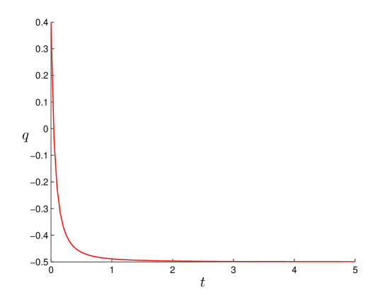
Figure 1: Plot of deceleration parameter $(q)$ versus time $(t)$.

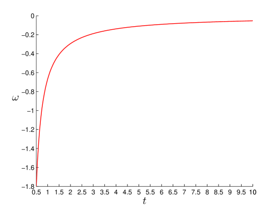
Figure 2: Plot of EoS parameter $(\omega)$ versus time $(t)$.

The sign of $q$ indicates whether the model inflates or not. A positive sign of $q$ corresponds to the standard decelerating model whereas the negative sign of $q$ indicates indicates inflation. The recent observations of SN Ia (Riess et al. 1998, Perlmutter et al. 1999) reveal that the present universe is accelerating and the value of DP lies somewhere in the range $-1<q<0$. Figure $1$ depicts the variation of DP versus cosmic time as representative case with appropriate choice of constants of integration and other physical parameters.
The energy density of the cosmic fluid $(\rho)$, EoS parameter $(\omega)$ and density parameter $(\Omega)$ are found to be

$$\rho=\frac{21(4t+\beta)^{2}}{16(4t^{2}+2\beta t+\gamma)^{2}}-\frac{1}{4(4t^{2}+2\beta t+\gamma)}$$ (32)

$$\omega=1-\frac{320(4t^{2}+2\beta t+\gamma)}{21(8t+2\beta)^{2}-16(4t^{2}+2\beta t+\gamma)}$$ (33)

$$\Omega=\frac{63}{64}-\frac{3(4t^{2}+2\beta t+\gamma)}{16(4t+\beta)^{2}}$$ (34)

From Eq. (33) follows that at large $t$ when only the quadratic terms stay alive, from EoS parameter we find

$$\omega\to 1-\frac{320.4t^{2}}{21.(8t)^{2}-16.4t^{2}}=1-\frac{320.4}{(21-1).64}=0,$$ (35)

i.e., under the present assumption the universe is ultimately filled with dust only at remote future.

The initial time of the universe is $t=\frac{-\beta+\sqrt{\beta^{2}-4\gamma}}{4}$. Therefore, at $t=\frac{-\beta+\sqrt{\beta^{2}-4\gamma}}{4}$, the spatial volume vanishes while all other parameter diverge. Thus the derived model starts expanding with big bang singularity at $t=\frac{-\beta+\sqrt{\beta^{2}-4\gamma}}{4}$ which can be shifted to $t=0$ by choosing $\gamma=0$. This singularity is point type because the directional scale factors $a_{1}(t)$ and $a_{2}(t)$ vanish at initial moment. The components of shear scalar vanish at $t\rightarrow\infty$. Thus in derived model the initial anisotropy dies out at later time.

Figure 2 depicts the variation EoS parameter $(\omega)$ versus cosmic time as representative case with appropriate choice of constants of integration and other physical parameters. It is shown that the growth of $\omega$ takes place with negative sign. It should be emphasized that there is a number of models for dark energy (quintessence, Chaplygin gas, phantom and many more) and quest for the right one is still going on. The main idea for the DE is a negative pressure, so one can try with a negative EoS parameter. It should be noted that the quintessence is given by a barotropic EoS only with negative parameter. We don’t call fluid a DE, we just construct DE in analogy with fluid. Figure 3 demonstrates the behavior of density parameter $(\Omega)$ versus cosmic time in the evolution of universe as representative case with appropriate choice of constants of integration and other physical parameters

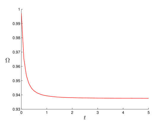
Figure 3: Plot of density parameter $(\Omega)$ versus time $(t)$.

4 Conclusion

In this paper, we have investigated LRS Bianchi II DE model under the assumption that $\vartheta\propto\sigma_{1}^{1}$. Under some specific choice of problem parameters the present consideration yields the variable DP and EoS parameter. It is to be noted that our procedure of solving the field equations are altogether different from what Pradhan et al (2011) have adapted. Pradhan et al (2011) have solved the field equations by considering the variation law for generalized Hubble’s parameter which gives the constant value of DP and only the evolution takes place either in accelerating or decelerating phase whereas we have considered the proportionality condition $\vartheta\propto\sigma_{1}^{1}$ in such a way that gives variable DP which evolves from decelerating phase to current accelerating phase (see Fig. 1). Thus the present DE model has transition of universe from the early deceleration phase to current acceleration phase which is in good agreement with recent observations (2006). The model has singular origin and the universe is ultimately filled with dust only at remote future.

The theoretical arguments suggest and observational data show, the universe was anisotropic at the early stage. Here we are dealing not only with the present state of the universe, but drawing a picture of the universe from the remote past to present day. We use the Bianchi model as one of many models able to describe initial anisotropy that dies away as the universe evolves. So though the model is anisotropic in the past for small t but it becomes isotropic as $t\rightarrow\infty$. In the derived model, the EoS parameter $(\omega)$ is evolving with negative sign which may be attributed to the current accelerated expansion of universe. Hence from the theoretical perspective, the present model can be a viable model to explain the late time acceleration of the universe. In other words, the solution presented here can be one of the potential candidates to describe the present universe as well as the early universe.

Acknowledgments

One of authors (AKY) is thankful to The Institute of Mathematical Science (IMSc), Chennai, India for providing facility and support where part of this work was carried out. Bijan Saha is thankful to joint Romanian-LIT, JINR, Dubna Research Project, theme no. 09-6-1060-2005/2013. Finally We would like to thank the anonymous referee for his valuable questions which helped us to understand the depth of the problem.

References

- [1] Adhav, K. S., et al: Astrophys. Space Sc. 331, 689 (2011)
- [2] Akarsu, Ö., and Kilinc, C. B.: Gen. Relativ. Gravit. 42, 119 (2010a)
- [3] Akarsu, Ö., and Kilinc, C. B.: Gen. Relativ. Gravit. 42, 763 (2010b)
- [4] Amendola, L.: Mon. Not. R. Astron. Soc. 342, 221 (2003)
- [5] Asseo, E., and Sol, H.: Phys. Rev. D 148, 307 (1987)
- [6] Astier, P., et al: Astron. Astrophys. 447, 31 (2006)
- [7] Bennett, C. L., et al: Astrophys. J. Suppl. Ser. 148, 1 (2003)
- [8] Caldwell, R. R., et al: Phys. Rev. D 73, 023513 (2006)
- [9] Caldwell, R. R.: Phys. Lett. B 545, 23 (2002)
- [10] Campanelli, L., Cea. P. and Tedesco, L.: Phys. Rev. D 97, 131302 (2006)
- [11] Campanelli, L., Cea, P. and Tedesco, L.: Phys. Rev. D 76, 063007 (2007)
- [12] Clocchiatti, A., et al: Astrophys. J. 642, 1 (2006)
- [13] de-Bernadis, P., et al: Nature 404, 955 (2000)
- [14] Eisentein, D. J., et al: Astrophys. J. 633, 560 (2005)
- [15] Ellis, G. F. R.: Gen. Relat. Gravit. 38, 1003 (2006)
- [16] Hanany, S., et al: Astrophys. J. 545, L5 (2000)
- [17] Hinshaw et al.: Astrophys. J. Suppl. 148, 135 (2003)
- [18] Hinshaw, G., et al: Astrophys. J. Suppl. 180, 225 (2009)
- [19] Hinshaw, G., et al: Astrophys. J. Suppl. 148, 135 (2009)
- [20] Hinshaw, G., et al: Astrophys. J. Suppl. 170, 288 (2007)
- [21] Hoftuft, J., et al: Astrophys. J. 699, 985 (2009)
- [22] Jaffe, J., et al: Astrophys. J. 629, L1 (2005)
- [23] Jaffe, J., et al: Astrophys. J. 643, 616 (2006a)
- [24] Jaffe, J., et al: Astron. Astrophys. 460, 393 (2006b)
- [25] Knop, R. K., et al: Astrophys. J. 598, 102 (2003)
- [26] Komatsu, E., et al: Astrophys. J. Suppl. Ser. 180, 330 (2009)
- [27] Kumar, S. and Akarsu, Ö.: arXiv: 1110.2408 [gr-qc] (2011)
- [28] Kumar, S. and Yadav, A. K.: Mod. Phys. Lett. A 26, 647 (2011)
- [29] MacTavish, C. J., et al: Astrophys. J. 647, 799 (2006)
- [30] Padmanabhan, T. and Raychowdhury, T.: Mon. Not. R. Astron. Soc. 344, 823 (2003)
- [31] Permutter, S., et al: Astrophys. J. 517, 565 (1999)
- [32] Pradhan, A., Amirhashchi, H. and Jaiswal, R.: Astrophys. Space Sc. 334, 249 (2011)
- [33] Riess, A. G., et al: Astron. J. 116, 1009 (1998)
- [34] Riess, A. G., et al: Astron. J. 607, 665 (2004)
- [35] Riess, A. G., et al: Astrophys. J. 560, 49 (2001)
- [36] Saha, B.: Cent. European J. Phys. 9, 939 (2011)
- [37] Seljak, et al: Phys. Rev. D 71, 043511 (2005)
- [38] Steinhardt, P. J., Wang, L. M. and Zlatev, I.: Phys. Rev. D 59, 123504 ( 1999)
- [39] Tegmark, M., et al: Phys. Rev. D 69, 103501 (2004)
- [40] Tonry, J. L., et al: Astrophys. J. 594, 1 (2003)
- [41] Yadav, A. K. and Yadav, L.: Int. J. Theor. Phys. 50, 218 (2011)
- [42] Yadav, A. K., Rahaman, F. and Ray, S.: Int. J. Theor. Phys. 50, 871 (2011)
- [43] Yadav, A. K.: Astrophys. Space Sc. 335, 565 (2011)
- [44] Yadav, A. K. and Saha, B.: Astrophys. Space Sc. 337, 759 (2012)