Factor models on locally tree-like graphs
Abstract
We consider homogeneous factor models on uniformly sparse graph sequences converging locally to a (unimodular) random tree , and study the existence of the free energy density , the limit of the log-partition function divided by the number of vertices as tends to infinity. We provide a new interpolation scheme and use it to prove existence of, and to explicitly compute, the quantity subject to uniqueness of a relevant Gibbs measure for the factor model on . By way of example we compute for the independent set (or hard-core) model at low fugacity, for the ferromagnetic Ising model at all parameter values, and for the ferromagnetic Potts model with both weak enough and strong enough interactions. Even beyond uniqueness regimes our interpolation provides useful explicit bounds on .
In the regimes in which we establish existence of the limit, we show that it coincides with the Bethe free energy functional evaluated at a suitable fixed point of the belief propagation (Bethe) recursions on . In the special case that has a Galton–Watson law, this formula coincides with the nonrigorous “Bethe prediction” obtained by statistical physicists using the “replica” or “cavity” methods. Thus our work is a rigorous generalization of these heuristic calculations to the broader class of sparse graph sequences converging locally to trees. We also provide a variational characterization for the Bethe prediction in this general setting, which is of independent interest.
doi:
10.1214/12-AOP828keywords:
[class=AMS]keywords:
, and t1Supported in part by NSF Grant DMS-11-06627. t2Supported in part by NSF Grant CCF-0743978. t3Supported in part by Dept. of Defense NDSEG Fellowship.
1 Introduction
Let be a finite undirected graph, and a finite alphabet of spins. A factor model on is a probability measure on the space of (spin) configurations of form
| (1) |
where is a symmetric function parametrized by , is a positive function parametrized by and is the normalizing constant, called the partition function (with its logarithm called the free energy). The pair is called a specification for the factor model (1).
In this paper we study the asymptotics of the free energy for sequences of (random) graphs in the thermodynamic limit . More precisely, with and denoting expectation with respect to the law of , we seek to establish the existence of the free energy density
| (2) |
and to determine its value. [In the literature, is also referred to as the “free entropy density” or “pressure.”]
The primary example we consider is the Potts model for a system of interacting spins on a graph. Formally, the -Potts model on with inverse temperature and magnetic field is the probability measure on (with ) given by
| (3) |
For the system favors monochromatic edges and is said to be ferromagnetic, while for the system favors edge disagreements and is said to be anti-ferromagnetic; the magnetic field biases vertices toward the distinguished spin . The -Potts model generalizes the Ising model which corresponds to the case . In analogy with the Potts model, in the general factor model setting we continue to refer to as the interaction or temperature parameter and to as the magnetic field.
Potts models have been intensively studied in statistical mechanics because of their key role in the theory of phase transitions MR641370 , critical phenomena MR1227790 and conformally invariant scaling limits MR2280251 . As demonstrated, for instance, in MR2875752 for the Ising model, determining the limit (2) plays a key role in characterizing the asymptotic structure of the measures in the thermodynamic limit. Potts models are also of great interest in combinatorics: recall in fact that the partition function admits a random-cluster representation (MR0359655 , MR2243761 ; see also Section 4.2), which at reads
with denoting the number of connected components induced by the subset of edges ; cf. (53). Up to a multiplicative constant this coincides with the Tutte polynomial of evaluated at , ; see, for example, MR2187739 .
Mathematical statistical mechanics has focused so far on specific graph sequences , for example, on finite exhaustions of the rectangular grid or other regular lattices in dimensions with fixed. Under mild conditions on the sequence, existence of the free energy density is a consequence of the following well-known argument (see, e.g., MR0289084 , Proposition 2.3.2): each graph can be decomposed into smaller blocks by deleting a collection of edges whose number is negligible in comparison with the volume. Consequently the sequence is approximately sub-additive in , implying existence of the limit; see MR0137800 .
In this paper we consider sparse graphs with a locally tree-like structure—formally, graph sequences converging locally weakly to (random) trees; see Definition 1.1 below; see also MR2354165 , MR1873300 . Although the study of statistical mechanics “beyond ” is not directly motivated by physics considerations, physicists have been interested in models on alternative graph structures for a long time (an early example being MR0436850 ). Moreover, the study of factor models on sparse graphs has many motivations coming from computer science and statistical inference; see MR2643563 , MR2518205 . Indeed, another example we will consider is the hard-core model for random independent sets on a graph. In this model the configuration space is , where means unoccupied, and means occupied, and the only configurations receiving positive measure are those for which no two neighboring vertices are occupied, that is, so that the occupied vertices form an independent set in the graph. Formally, the independent set or hard-core model on with fugacity is the probability measure on given by
| (4) |
so that as increases the measure becomes more biased toward the larger independent sets (and we write for the magnetic field). Due to the hard constraint preventing neighboring s, this system always has anti-ferromagnetic interactions and is of significant interest in computer science. The independent set decision problem is np-complete (via the clique decision problem Cook1971CTP800157805047 , MR0378476 ). As increases the measure becomes increasingly concentrated on the maximal independent sets; the optimization problem of finding such sets is np-hard MR584512 and hard to approximate (Zuckerman2006LDE11325161132612 and references therein). The problem of counting independent sets [i.e., computing ] for graphs of maximum degree is #p-complete for (MR1791090 and references therein). Although there exists a ptas (polynomial-time approximation scheme) for for below a certain “uniqueness threshold” MR2277139 , a series of previous works (see MR2475668 , 101109FOCS201034 , springerlink101007978364222935048 and references therein) gave strong evidence that computation is hard for any above this threshold. This question was resolved simultaneously in the subsequent works arXiv12032226 , arXiv12032602 , with arXiv12032602 building on methods from this paper.
Since infinite trees are nonamenable, cannot be decomposed by removing a vanishing fraction of edges, so the preceding argument no longer applies: in physics terms, surface effects are nonnegligible even in the thermodynamic limit. Despite this, statistical physicists expect the free energy density (2) to exist on a large class of locally tree-like graphs. Even more surprisingly, employing nonrigorous but mathematically sophisticated heuristics such as the “replica” or “cavity” methods, they derive exact formulas for this limit for a number of statistical mechanics models on locally tree-like graphs; see, for example, MR2518205 and the references therein. The primary example considered in these works is the graph chosen uniformly at random from those with vertices and edges, with ; such graphs converge locally to the Galton–Watson tree with offspring distribution. The Galton–Watson tree with general offspring distribution can be obtained as the local weak limit of random graphs with specified degree profile corresponding to the offspring distribution; the physics heuristics extend to this and even more general settings.
There is no good argument for why the limit (2) exists; the heuristic replica or cavity methods compute this limit starting from the postulate that it exists. A significant breakthrough was achieved by the interpolation method first developed by Guerra and Toninelli MR1930572 for the Sherrington–Kirkpatrick model from spin-glass theory, and then generalized to a number of statistical physics models on sparse graphs MR1972121 , MR2025238 , MR2095932 and related constraint satisfaction problems MR2743259 . This method establishes super-additivity of which implies existence of the limit (2). Unfortunately, this approach appears limited to models with repulsive interactions, that is, in which higher weight is given to configurations in which neighboring vertices take different values. In particular, it does not apply to the ferromagnetic Potts model. This is especially puzzling because the heuristic physics predictions do not distinguish between the two cases, and there is no fundamental reason why the limit should be computable in one case and not in the other. Further, this interpolation method only applies to very restricted classes of graph sequences (typically, uniformly random given the degree sequence); notably, existence of the limit is not proved for deterministic graph sequences. Finally, the method gives no way to actually compute the limit, although interpolation has been used to prove upper bounds MR1972121 , MR2025238 , MR2095932 .
In this paper we follow a different approach relying only on local weak convergence of the graph sequence to some limiting (random) tree. The general idea is that the corresponding factor models (1) must converge (passing to a subsequence as needed), to a Gibbs measure on the limiting tree; the task then “reduces” to the one of identifying the correct limit. This is still a substantial challenge because, in general, there is an uncountable number of “candidate” Gibbs measures for the limit. Nevertheless, this program was carried through in MR2650042 for Ising models on graphs converging locally to a Galton–Watson tree, under a “uniform sparsity” assumption (Definition 1.3), on the degree distribution. (It is further assumed in MR2650042 that the distribution has finite second moment; this condition was relaxed in MR2733399 , thereby handling the case of power law graphs.) The result of MR2650042 , MR2733399 provides also a fairly explicit expression for the free energy density, defined solely in terms of the limiting tree. This expression coincides with the so-called “Bethe prediction” of statistical physics, derived earlier for random graphs with given degree distribution using the “replica” or “cavity” methods.
We develop this approach here in more generality. Rather than considering a specific model such as the Ising, we establish results for general abstract factor models satisfying mild regularity conditions [see (H1) below], covering in particular the Potts and independent set models. We also make no distributional assumptions on the graphs or the limiting random tree, other than some integrability conditions [see Definition 1.3 and (H2) below]. In this setting we develop a general interpolation scheme (Theorem 1.15) which, under appropriate assumptions, bounds differences in the limit by differences for a functional defined solely in terms of the limiting tree; see (13). We refer the reader to MR2023650 for a discussion of the computation of limits of finite large random structures through optimization procedures on the limiting infinite structure. Although we continue to refer to this as the “Bethe prediction,” we remark that it is a considerable generalization of earlier formulas obtained in the special case of Galton–Watson trees by statistical physics methods. It is defined as the evaluation of the “Bethe free energy functional” (10) at a specific Gibbs measure on the limiting tree, and corresponds to what physicists call the “replica symmetric solution”: whereas it is expected to hold in the high-temperature regime (i.e., with small enough interactions), for many factor models it is incorrect at low temperature. However, we will show that in “uniqueness regimes,” where the set of Gibbs measures on the limiting tree corresponding to the factor model specification is a singleton, the upper and lower bounds of Theorem 1.15 match to completely verify the Bethe prediction (Theorem 1.16).
We then apply our interpolation scheme to compute the free energy density in specific models. We verify the Bethe prediction for the independent set model with low fugacity (Theorem 1.12) as a consequence of Theorem 1.16. Further, by using monotonicity properties to restrict the set of relevant Gibbs measures, we obtain results for the Potts model going beyond the implications of Theorem 1.16: for (Ising), we verify the Bethe prediction for all , (Theorem 1.9), extending the results of MR2650042 , MR2733399 to general locally tree-like graph sequences. For general , we verify the prediction in regimes of nonnegative in which two specific Gibbs measures on the limiting tree coincide, namely, the Gibbs measures arising from free and 1 boundary conditions coincide, see Definition 1.8 below. This condition is satisfied throughout the range for ; when there are regimes of nonuniqueness in which it fails, but we will show that it is satisfied both at sufficiently small and sufficiently large, that is, at high and low temperatures.
Theorem 1.15 can give useful bounds even beyond uniqueness regimes. As an illustration, we study the Potts model in the case that converges locally to the -regular tree . In Theorem 1.11 we explicitly characterize the nonuniqueness regime of this model and use Theorem 1.15 to give bounds for within this regime. In a subsequent work arXiv12075500 we prove that in this setting, exists and matches the lower bound of Theorem 1.11. We also compute there the asymptotic free energy (all ) for the independent set model on -regular bipartite graphs. In contrast, for generic nonbipartite the consensus in physics is for a full replica symmetry breaking for large enough , and consequently there does not exist even a heuristic prediction for the free energy density in this regime.
As mentioned above, the Bethe prediction is the evaluation of the Bethe free energy functional at a specific Gibbs measure on the limiting tree. This Gibbs measure has a characterization in terms of “messages” defined on the directed edges of each tree , such that the entire collection of messages is a fixed point of a certain “belief propagation” or “Bethe recursion” (1.6). Motivated by the finite-graph optimization of MR2246363 , we provide a variational characterization of the Bethe prediction (Theorem 1.18) which is of independent interest. In particular, this formulation suggests nontrivial connections with large deviation principles.
1.1 Local weak convergence and the Bethe prediction
We study factor models on graphs which are “locally tree-like” in a sense which we now formalize, starting with a few notation and conventions. All graphs are taken to be undirected and locally finite. In a graph , let denote graph distance, and for write for the sub-graph of induced by . Write if are neighbors in , and write for the set of neighbors of and . Let denote the space of isomorphism classes of (finite or infinite) rooted, connected graphs . A metric on this space is given by defining the distance between and in to be where is the maximal such that ; with this definition is a complete separable metric space; see, for example, MR2354165 . Let denote the closed subspace of (rooted) trees , the acyclic elements of . We write for in , and in particular we use to denote the single-vertex tree. We now define the precise notion of graph limits considered throughout this paper.
Definition 1.1.
Let () be a sequence of random graphs, and let be a vertex chosen uniformly at random from . We say converges locally (weakly) to the random tree if for each , converges in law to in the space . We say in this case that the are locally tree-like.
We will make repeated use of the fact that any local weak limit of graph sequences satisfies the “unimodularity” or “mass-transport” property whose definition we recall here; for a detailed account, see MR2354165 . Let denote the space of isomorphism classes of bi-rooted, connected graphs with a distinguished ordered pair, denoted (we do not require ); is metrizable in a similar manner as .
Definition 1.2.
A Borel probability measure on is said to be unimodular if it obeys the mass-transport principle,
| (5) | |||
| (6) |
We say that is involution invariant if (1.2) holds when restricted to supported only on those with .
A measure on is involution invariant if and only if it is unimodular (MR2354165 , Proposition 2.2). Unimodularity corresponds to “indistinguishability of the root;” the concept first appeared in MR1873300 where it was observed that local weak limits of graph sequences must be unimodular (MR1873300 , Section 3.2). The converse of this implication remains a well-known open question; see MR2354165 .
Definition 1.3.
The graph sequence is uniformly sparse if the are uniformly integrable, that is, if
(where denotes expectation over the law of and ).
We assume throughout that () is a uniformly sparse graph sequence converging locally weakly to the random tree of (unimodular) law such that the root degree is nonzero with positive -probability; this entire setting is hereafter denoted . In this setting we will describe general conditions under which the asymptotic free energy for the factor model (1) exists and agrees with the “Bethe energy prediction,” which we now describe. [If the sequence of random graphs is such that for almost every realization of the sequence—as is the case for Erdös–Rényi random graphs or random graphs with given degree distribution (see, e.g., MR2643563 , Propositions 2.5 and 2.6)—then our results apply instead to the a.s. limit of .]
Let denote the -dimensional simplex of probability measures on the finite alphabet of spins . Let denote without the single-vertex tree , and let be the space of isomorphism classes of trees rooted at a directed edge , written or simply for short. If has law for a unimodular measure on , we let and denote the laws of and , respectively, for chosen uniformly at random from conditioned on the event . Involution invariance of is then equivalent to
(where corresponds to on the left-hand side and to on the right-hand side), so in particular and are mutually absolutely continuous.
Definition 1.4.
The message space is the space of measurable functions
taken up to -equivalence.
Remark 1.5.
For let denote the component sub-tree rooted at which results from deleting edge from . The interpretation of is that it is a message from to on the tree , giving the distribution of for the factor model (1) on . Indeed, although we do not require it in general, in our concrete examples depends only on this component sub-tree.
For and , let
where “” and “” indicate vertex and edge terms, respectively:
| (8) |
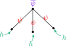
the log-partition function of the star graph with boundary conditions [see Figure 1(a)] and
half the log-partition function on disjoint edges with boundary conditions ; see Figure 1(b). (See Definition 1.8 below for a detailed discussion of boundary conditions.)
 |
|
| (a) Star graph | (b) Edge graph |
We take the usual convention that the empty sum is zero, and the empty product is one, so in case . Although we suppress it from the notation, in the above equations and are taken to be evaluated at . The Bethe free energy functional on for the factor model (1) on is defined by
| (10) |
provided the expectation exists; see Lemma 2.2.
Definition 1.6.
The belief propagation or Bethe recursion is the mapping ,
| (11) | |||
with normalizing constants. For a measure on and fixed , let denote the space of measurable functions , again taken up to -equivalence, which are fixed points of the Bethe recursion: that is, satisfying
| (12) |
The Bethe prediction is that the asymptotic free energy of (2) exists and equals
| (13) |
for a certain element of . We often drop the subscript when it is clear from context.
Remark 1.7.
In the case that the recursion (12) has multiple solutions (), the Bethe prediction is defined to be the supremum of over admissible fixed points . While in the abstract factor model setting all fixed points are admissible, in specific models typically there are “natural” criteria restricting the set of admissible fixed points. We will demonstrate this in the Ising and Potts models where restrictions are imposed by monotonicity and symmetry considerations.
The rationale behind the Bethe recursions and Bethe prediction is explained in detail in MR2643563 , Section 3; see also MR2518205 . In brief, solutions to the Bethe recursions correspond to consistent “boundary laws” for the factor model on tree-like graphs; for further details, see Remark 1.13 below. When is a finite tree, and is the law of for a uniform element of (here is a measure on , but not necessarily unimodular), the Bethe recursions have a unique solution, given by the so-called “standard message set;” see MR2643563 , Remark 3.5. In this setting it holds exactly (see MR2643563 , Proposition 3.7) that
where is as defined by (1.1) with . The heuristic then is that for locally like the random tree , the (normalized) free energy is approximated by for large. We emphasize that no averaging over the vertices of the tree takes place in the definition of ; indeed for the sub-trees typically do not converge locally weakly to . For example, when is the -regular tree , the subtrees converge locally weakly to the so-called -canopy tree; see, for example, MR2643563 , Lemma 2.8. Instead the averaging of over the vertices in the evaluation of corresponds to the averaging with respect to the law in the evaluation of the Bethe prediction .
The following is a terminology which we adopt throughout the paper:
Definition 1.8.
If is any graph and a sub-graph, the external boundary of is the set of vertices of adjacent to . Let denote the sub-graph of induced by the vertices in . For finite (so is finite, since is locally finite), and a measure on , the factor model on with boundary conditions is the probability measure on configurations given by
| (14) |
(Throughout, indicates equivalence up to a positive normalizing constant.) The case in which gives probability one to the identically- spin configuration on () is referred to as boundary conditions and denoted , while the case in which is uniform measure on is referred to as free boundary conditions and denoted .
1.2 Application to Ising, Potts and independent set
Before formally stating our main theorem for general factor models, we mention its consequences in some models of interest: we verify the Bethe prediction for the ferromagnetic Ising model at all temperatures, the ferromagnetic Potts model with field in uniqueness regimes, and the independent set model with low fugacity .
1.2.1 Ising model
The Ising model is the Potts model (3) with . For convenience we use the equivalent formulation which takes and defines the probability measure on
| (15) |
For let denote the root marginal for the Ising model of parameters on with boundary conditions (i.e., with conditioned to be for all at level ), and similarly define corresponding to free boundary conditions. For let . (Existence of the limits for the Ising model is an easy consequence of Griffiths’s inequality; see Lemma 4.1.) We then define messages by
for as defined in Remark 1.5. For , the Bethe free energy prediction for the Ising model with , is . This prediction was verified in MR2650042 , Theorem 2.4, for uniformly sparse graph sequences converging locally weakly to Galton–Watson trees subject to the second-moment condition , which was relaxed in MR2733399 to a -moment condition. We have the following generalization of this result to an arbitrary limiting law.
Theorem 1.9
Note that in the Ising model we are able to characterize the free energy density for all . The underlying reason is that for , all boundary conditions dominating the free boundary condition give rise to the same Gibbs measure on the limiting tree, that is, . This phenomenon appears to be in line with physicists’ intuition that the Ising model always undergoes a second-order phase transition. The physics argument suggests therefore that the zero-magnetization phase becomes unstable below the critical temperature. In other words, even with free boundary conditions, an arbitrarily small external field is sufficient to drive the system into the “plus” phase.
1.2.2 Potts model
Throughout the remainder let , where means coordinate-wise less than or equal to. An interpolation path is a piecewise linear path, with each piece parallel to a coordinate axis, increasing from to with respect to the partial order .
We restrict our attention to the Potts model with . In this regime we are able to use a random-cluster representation to extract important monotonicity properties. For and let denote the root marginal for the Potts model on with boundary conditions. Let (existence of the limits for the Potts model follows from monotonicity properties of the random-cluster representation; see Corollary 4.4). We then define messages by , and let
We also define
Theorem 1.10
For the Potts model (3) with and on , the following hold (with , ): {longlist}[(a)]
If there exists an interpolation path contained in joining and , then
If there exists an interpolation path from to along which is continuous (in the interpolation parameter), then
If is replaced with , then we have instead
We obtain more explicit results when the limiting tree is the -regular tree .
Theorem 1.11
For the Potts model (3) with and on , the following hold (with , , and ):
[(a)]
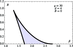
If , . If and , there exists such that . If and , there exists and smooth curves defined on with such that
For , . If with , then . If with , then . For in the interior of ,
where
 |
 |
| (a) Ising | (b) Potts |
 |
 |
| (a) BP fixed points | (b) Regime (shaded) |
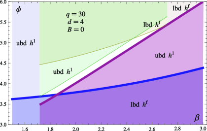
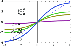
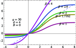
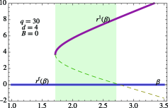
Figures 2–4 highlight the difficulty in analyzing the Potts model () as opposed to the Ising model. Figure 2(a) shows the Ising Bethe recursion parametrized in terms of the log-likelihood ratio . For sufficiently large the recursion has three fixed points, but in this case the fixed point is unstable, and we will see in the proof of Theorem 1.9 that adding a small magnetic field resolves the nonuniqueness. The remaining plots were computed for the Potts model with and . Figure 2(b) shows the Potts Bethe recursion at restricted to those which are symmetric among the spins , and parametrized by . The fixed point at corresponds to while the uppermost fixed point corresponds to ; Figure 3(a) shows how the fixed points vary with . In an intermediate regime of -values [shaded in Figure 3(a)] both fixed points are stable, and perturbing by a magnetic field does not resolve the nonuniqueness: indeed, Figure 3(b) shows that there is a two-dimensional region of values for which , making the exact Bethe prediction inaccessible via our current interpolation scheme. Figure 4 shows the discrepancy between the upper and lower bounds of Theorem 1.11(b) inside .
1.2.3 Independent set model
We consider the independent set model (4) in the regime of low fugacity. For let denote the root marginal on with boundary conditions on : that is, (resp., ) is calculated conditional on the event of being fully occupied (unoccupied) at level of . Let (existence of the limits for the independent set model follows from anti-monotonicity; see Section 2.4). We then define messages by , and let
denote the uniqueness threshold. For we write
(where the limit is taken over cutsets of with distance from the root tending to infinity) for the branching number of ; see MR1062053 , Section 2.
Theorem 1.12
Consider the independent set model (4) on , and write . {longlist}[(a)]
If and the function has total variation bounded by a deterministic constant on , then
| (17) |
which converges to as .
If -a.s. for a deterministic constant, then (17) holds for with .
If , then (17) holds for .
For the -regular tree , the uniqueness threshold is (see MR844469 , Section 2), and MR2277139 , Theorem 2.3, shows that has the lowest value of among trees with maximum degree at most . The identity (17) has been proved in the case that the are random -regular graphs MR2373815 , MR2462251 . It is also suggested by Weitz’s ptas for on a finite graph of maximum degree and with (MR2277139 , Corollary 2.8). For a unimodular measure on giving a local tree approximation to (in the sense of Definition 1.1), is often an improvement over , making it possible to compute above provided (H3B) can be verified. In arXiv12032602 the interpolation scheme of Theorem 1.12 is refined to give a verification of the Bethe prediction on locally tree-like -regular bipartite graphs for all ; this result is then leveraged to show inapproximability of the hard-core partition function on -regular graphs above .
1.3 Results for general factor models
We now state our results for the factor model (1). With the convention , let and , and impose the following regularity condition: {longlist}
The specification is permissive, that is, for all , and there exists a “permitted state” such that .
For any , is continuously differentiable in . For any , is either identically over all , or finite and continuously differentiable in . Recalling Definition 1.4 of the message space , for we can define up to -equivalence by
| (18) |
In particular, if and , then comparing (18) with (1.6) gives
| (19) |
independently of the choice of . From now on, for , we will write to indicate that for in the range being considered.
Remark 1.13.
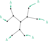
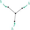
The elements of are consistent with the recursion structure of the tree in the following precise sense: for and a finite connected sub-graph of , consider the factor model on with boundary conditions independently for , where denotes the (necessarily unique) neighbor of inside . Then the marginal of on is exactly the factor model on with boundary conditions independently for , including any which are leaves of . This statement remains valid if or even is empty, since if then is simply as defined by (1). Continuing the recursion up the tree, we see that implies that the marginal law of will be as defined by (18). From this it is easy to see that the measures form a consistent family of finite-dimensional marginals (see Figure 5), so by the Kolmogorov consistency theorem they uniquely determine a probability measure belonging to , the set of Gibbs measures (or Markov random fields) associated to the specification on .444Strictly speaking the term “Gibbs measures” refers to the case , but we will follow common practice and say Gibbs measures also for the general case. For the general theory of Gibbs measures see, for example, MR956646 . (In fact this mapping is one-to-one, e.g., by Remark 2.3 below.) Each belongs to a special class of measures in which are called Markov chains or splitting Gibbs measures in the literature, and the entire collection arising from has a consistency property which leads us to term them “unimodular Markov chains” or “Bethe Gibbs measures;” see Section 2.3.
 |
 |
| (a) | (b) |
In this general setting, the Bethe prediction is the supremum of over ; cf. Remark 1.7. (It will be shown in Lemma 2.2 that is uniformly bounded on subject to ; if further , then is in fact uniformly bounded on subject only to .) We define the following integrability condition for unimodular measures on (not necessarily arising from a graph sequence): {longlist}[(H2)]
The probability measure on satisfies . If is not everywhere positive, then furthermore for all . Note that if and , then (H2) holds trivially by the assumption of uniform sparsity. We will in fact justify our interpolation scheme under a weaker assumption than (H2); for the exact condition see (H2β), (H2B) in Section 2.2.
1.3.1 Bethe interpolation
We will deduce the results of Section 1.2 from the abstract interpolation method given by Theorem 1.15 below, which bounds differences of by differences of () when the limiting expectation of a certain edge or vertex functional in the finite graph (capturing resp. or ) is bounded by the expectation of an analogous functional on the infinite tree.
To be more precise, recall that denotes a uniformly random vertex of . Let denote expectation with respect to , conditioned on . For and , let denote expectation with respect to (as defined in Remark 1.13), conditioned on , and define
The left-hand side expressions are the derivatives , (Lemma 2.1). The right-hand side expressions are the infinite-tree analogues, which, as we will show in Proposition 2.4, may be thought of as derivatives in and of .
Example 1.14.
For example in the Potts model (3) we have , so is the expected density of s in the graph while is times the expected number of edge agreements, both with respect to the Potts measure on . The infinite tree analogues of and are
the -probability (averaged over ) that the root spin takes value and
the -expectation (averaged over ) of half the number of edge agreements incident to the root.
For interpolation in on a compact interval using some particular , we require the following regularity condition on : {longlist}
On , for all it holds -a.s. that the function is continuous with total variation in bounded by a deterministic constant depending only on . Likewise for interpolation in on a compact interval using we require {longlist}
On , for all it holds -a.s. that the function is continuous with total variation in bounded by a deterministic constant depending only on . The condition of boundedness in total variation is implied for example whenever the functions are (anti-)monotone in the interpolation parameter.
Theorem 1.15
Let specify a factor model (1) on such that (H1) and (H2) are satisfied. {longlist}[(a)]
If on we have satisfying (H3β), and
| (20) |
then .
If on , we have satisfying (H3B), and
| (21) |
then . The same results hold if all inequalities are reversed, replacing limit superior with inferior.
Conditions (20), (21) (and their reverses) are automatically verified in the following special case, where we recall that denotes the set of Gibbs measures associated to the specification on ; cf. Remark 1.13:
Theorem 1.16
Let specify a factor model (1) on satisfying (H1) and (H2). We say that uniqueness holds if at consists of a single measure , -a.s. In this case, is a singleton.
[(a)]
If on uniqueness holds and the unique element satisfies (H3β), then
If on uniqueness holds and the unique element satisfies (H3B), then
Uniqueness for corresponds to the vanishing effect of boundary conditions on as (MR956646 , Chapter 7). Dobrushin’s uniqueness theorem (see, e.g., MR543198 ) gives a sufficient condition for uniqueness to hold, together with a bound on the rate of convergence of the root marginal in to the limit as . Note that if the convergence rate is uniform in then the continuity required in (H3β) and (H3B) immediately follows. We will obtain continuity in uniqueness regimes via a different route, making use of certain monotonicity properties; see the proof of Theorem 1.9.
1.3.2 Variational principle
We further develop the theory by providing a variational principle for the Bethe prediction: we express as an optimum of a function defined for in a larger space which, unlike , is independent of . This alternative characterization of is the infinite-tree analogue of the finite-graph optimization problem that is considered in MR2246363 . Recall from Section 1.1 that denotes the space of trees rooted at a directed edge.
Definition 1.17.
The local polytope is the space of measurable functions
taken up to -equivalence, such that: {longlist}[(ii)]
for all , and
for , the one-point marginal is well-defined, that is, does not depend on the choice of . We also define
In accordance with (18), we set
| (22) |
For fixed , by symmetry of and (19), the space has a natural mapping into given by
| (23) |
With permissive this is in fact an embedding; see Remark 2.3. We define the Bethe free energy functional on by
where denotes the Shannon entropy for a probability measure on a finite space. This is an infinite-tree analogue of the definition of MR2246363 , (37)–(38), for finite graphs. With the usual conventions , and , is bounded above on whenever , and we show in Lemma 3.1 that for unimodular, this extends the previous definition (10) on [under the embedding (23)], provided the latter is finite. Furthermore, writing for the relative entropy between and (well defined for any nonnegative reference measure ), for unimodular we can alternatively express
| (26) |
where , and unimodularity is used in the second identity.
This extended definition of provides the following variational principle for the Bethe free energy:
Theorem 1.18
Let specify a factor model (1) satisfying (H1), and let be a unimodular measure on with . {longlist}[(a)]
is continuous in .
Any local maximizer of belongs to . Any stationary point of belonging to is the image under (23) of an element of . In particular, if attains its supremum on , then
so that the Bethe free energy is also continuous in .
Although we do not pursue this point, we mention that even in specific models where the abstract definition of is supplanted by for some “naturally” distinguished , an adaptation of Theorem 1.18 [involving a restricted subspace of which is independent of ], may be relevant.
Remark 1.19.
In case the -regular tree, is parametrized by a single measure on whose one-point marginals are required to agree, and the formula (26) simplifies to
| (27) |
For let and denote the induced empirical and pair empirical measures, respectively. If is -regular, then the one-point marginals of coincide with , and
where the law of is the uniform measure on and denotes expectation with respect to (with fixed).
If is an independent sequence of uniformly random -regular graphs and , one might guess that for a.e. the induced sequence satisfies a large deviation principle (ldp) with good rate function
| (28) |
where . If this were the case, it would be an immediate consequence of Varadhan’s lemma (see MR1619036 , Section 4.3.1) that (as defined in Theorem 1.18) for any factor model satisfying (H1). However, for many of these models the Bethe prediction is known to fail at low temperature for . So, while Theorem 1.18 suggests a potential connection to large deviations theory, such a connection would be highly nontrivial and applicable only in certain regimes of .
One special case in which everything trivializes is the (rooted) infinite line , the local weak limit of the simple path on vertices. In this case may be viewed as the law of a stationary reversible Markov chain on with transitions and reversing measure , and it is well-known (see, e.g., MR1619036 , Theorem 3.1.13) that the associated pair empirical measure satisfies an ldp with good rate function which matches (28). The implication of Varadhan’s lemma is also easy to see: a factor model on the simple path with general positive specification corresponds in the limit to a reversible Markov chain with transition kernel and positive reversing measure given by
where and are the Perron–Frobenius eigenvalue and eigenvector of the symmetric positive -dimensional matrix with entries . The Bethe free energy functional (27) is then maximized at , where it takes the value which coincides with by the Perron–Frobenius theorem; see, for example, MR1619036 , Theorem 3.1.1.
Outline of the paper
-
•
In Section 2 we prove the abstract interpolation results. Section 2.1 presents some preliminary lemmas which will be useful in our proofs. Our main result for abstract factor models, Theorem 1.15, is proved in Section 2.2. Section 2.3 contains the specialization of this theorem to the uniqueness case (Theorem 1.16) and also contains discussion on unimodular Markov chains (or Bethe Gibbs measures). Section 2.4 shows how to deduce our result for independent set (Theorem 1.12) from Theorem 1.15.
-
•
In Section 3 we prove the variational characterization Theorem 1.18 for the Bethe free energy prediction, establishing in particular the correspondence between interior stationary points of and fixed points of the Bethe recursion. We further provide in Proposition 3.4 a simple criterion for such stationary points to be local maximizers.
-
•
Section 4 contains applications of our abstract results to the Ising and Potts models. In Section 4.1 we prove Theorem 1.9, generalizing the results of MR2650042 , MR2733399 . In Section 4.2 we prove Theorem 1.10 by appealing to a random-cluster representation. Finally, Section 4.3 analyzes the -regular case and proves Theorem 1.11.
2 Bethe interpolation for general factor models
2.1 Preliminaries
We begin with some straightforward observations on the boundedness of the free energy and the Bethe free energy as defined on , and we prove that the mapping (23) of into is in fact an embedding for permissive specifications.
Lemma 2.1
For the factor model (1) satisfying (H1) on , the functions are uniformly bounded and equicontinuous on compact regions of , with
Further,
with the convention in case .
The expressions for and are obtained by a straightforward computation. Now note that if , then the uniform sparsity assumption gives
| (30) |
Let vary within a given compact region. By (H1) we have as well as . Therefore,
so is uniformly bounded by uniform sparsity. The exchange of differentiation and integration in (2.1) is justified by Vitali’s convergence theorem, in view of the boundedness of , and the uniform integrability of . It follows furthermore that and are bounded uniformly in , from which equicontinuity follows.
Lemma 2.2
Let specify a factor model (1) satisfying (H1), and let be a unimodular measure on . For any compact region of there exists a deterministic constant such that: {longlist}[(a)]
for any , and
if further , then for any . Hence, on any compact region of , is uniformly bounded on provided , and if , uniformly bounded on subject only to .
Let be as in the proof of Lemma 2.1. Then, for any ,
If , then we also have
so on , which proves (b). For general permissive , the preceding lower bound on may fail, but (12) implies that for ,
| (31) |
Therefore,
which proves (a).
Remark 2.3.
It is now easy to see that the mapping (23) of into is injective: if give rise to the same , then
for a positive scaling factor. If , then (31) implies that -a.s. both and give positive measure to . Therefore, -a.s. the -dimensional vectors and are equivalent up to scaling, and since both are probability measures on , we must have -a.s. as claimed.
2.2 Bethe interpolation
We now prove Theorem 1.15(a). The result is for fixed , so we suppress it from the notation. The proof of Theorem 1.15(b) is very similar and will be given in brief at the end of this section.
Our interpolation procedure relies on the proposition below which expresses as the integral of its partial derivative with respect to only, ignoring the dependence on through the function . Recall that although it is suppressed from the notation, and depend on , and are taken to be evaluated at in expressions such as . We will prove our result under the following integrability condition, which by (31) is a relaxation of (H2): {longlist}
The probability measure on satisfies . If is not everywhere positive, then furthermore,
We define the analogous condition (H2B) on an interval .
Proposition 2.4
Let be a specification satisfying (H1), and a unimodular measure on . If on we have satisfying (H2β) and (H3β), then
For fixed we shall regard simply as a function of a vector in -dimensional euclidean space (with depending on ). We begin by computing the partial derivatives of this function with respect to and . We abbreviate for the belief propagation mapping of (1.6), which for fixed and each is a well-defined function on the same euclidean space as . Making use of (H1) we find
| (32) | |||||
| (33) |
If , then , therefore (recalling the notation from Section 1.3.1) we re-express the above as
and combining gives
| (34) |
Likewise we compute that for ,
where is the same as but with in place of . Note that for permissive and any ,
| (35) |
If further everywhere, then is uniformly bounded on .
Consider now a small sub-interval of . Writing and applying the mean value theorem to the differentiable function for gives
| (36) | |||
for some , where
and indicates the sum over the directed edges within .
Setting , we now sum over and analyze separately the contribution of each term on the right-hand side of (2.2):
[(a)]
First we show that for any . Indeed, since we have and . Therefore,
The result then follows from unimodularity of , subject to -integrability of
Clearly so integrability certainly holds when , since and is deterministically uniformly bounded on as noted above. More generally, for permissive the required -integrability follows from (35) and (H2β).
The total contribution of the first term on the right-hand side of (2.2) is
Observe that where is Lebesgue measure on and
For -a.e. , this sum has at most one nonzero term, in which the argument of converges by (H3β) to as . From (H1), (1.6) and the computation of in (32)–(33), we see that is continuous in . Therefore, , -a.e. Furthermore, (H1) implies that uniformly on for some deterministic constant , so for all , -a.e. see (32) and (33). Dominated convergence then gives
Indeed, it is not hard to see that -a.s.: by the uniform bound on total variation assumed in (H3β), there exists deterministic such that
-a.s., uniformly in . It also follows from (H3β) that -a.e. is uniformly continuous on . Using (H1), the partials computed above are uniformly continuous in for and uniformly bounded away from zero. By (31) there exists deterministic such that
Combining these observations gives -a.s.
To take the limit in -expectation, we argue similarly as in part (a): by (35) and (H1) there exists deterministic such that
for all , , and , hence
This is integrable by (H2β) and unimodularity of , so dominated convergence implies that as claimed. Combining (a)–(c) gives the result of the proposition.
Proof of Theorem 1.15(a) Recalling Lemma 2.1,
where the first inequality follows by (the reversed) Fatou’s lemma and the second one by the hypothesis (20). By Proposition 2.4 the right-most expression equals to , so the theorem is proved.
The justification for interpolation in is entirely similar:
2.3 Discussion and first consequences
We now prove Theorem 1.16 by considering an extended notion of local weak convergence. As discussed in MR2354165 , a graph together with a spin configuration on the graph can be regarded as a graph with marks in . Let and denote the spaces of marked isomorphism classes of connected, rooted and bi-rooted graphs, respectively, with marks in . These spaces are metrizable by the obvious generalizations of the metrics on defined in Section 2.1, giving rise to the notion of local weak convergence for pairs of graphs with spin configurations. Definition 1.2 generalizes naturally to this setting, and we show next that if is a random configuration on with law [as defined in (1)], then a local weak limit of , if it exists, must be unimodular.
Lemma 2.5
If and , then the laws of have subsequential local weak limits belonging to the space of unimodular measures on .
For each fixed , the laws of are weakly convergent, hence by Prohorov’s theorem form a uniformly tight sequence. Consequently, for each there exists compact with . Further, may be taken to contain only graphs of depth at most , whereby the minimal distance between any two graphs in is uniformly bounded below [by ], hence the compactness of implies that it must be a finite set. The collection of all marked graphs in whose underlying graph is in must therefore be finite, hence compact as well. Thus, by yet another application of Prohorov’s theorem, the joint laws of are uniformly tight in and consequently have subsequential weak limits. By extracting successive subsequences for increasing and taking the diagonal subsequence, it follows that the sequence admits subsequential local weak limits .
For , the marginal of is a unimodular measure on . If it is supported on a single tree as in the -regular case, then clearly may be represented as where , the space of Gibbs measures on corresponding to specification . To make such a statement in the general setting, note that there is a continuous mapping from to the space of graphs on rooted at , taking an isomorphism class to its canonical representative (MR2354165 , page 1461). Thus may be regarded as a measure on the product space , and consequently has a representation as the measure on pairs where has law and given has law . In particular, if -a.s., then is uniquely determined.
Let be a unimodular measure on . It was noted in Remark 1.13 that there is a mapping from to collections . For such , belongs to : if is a nonnegative Borel function on , it follows from the -measurability of elements of that
where is a nonnegative Borel function on . The unimodularity of the underlying measure then gives
and therefore .
Remark 2.6.
An element is called a Markov chain (or splitting Gibbs measure) if for any finite connected sub-graph , the marginal of on is a Markov random field MR714953 ; see also MR956646 , Chapter 12, and MR0378152 . A collection of probability measures on is called an entrance law (or boundary law) for the specification on if it satisfies the consistency requirement (MR714953 , (3.4))
where , the pairwise interaction potential corresponding to . It is shown in MR714953 , Theorem 3.2, that there is a one-to-one correspondence between Markov chains and entrance laws , given by
for any finite connected sub-graph of , with denoting the unique neighbor of inside for . In particular, we see that the Gibbs measure arising from is precisely the Markov chain with entrance law . Extremal elements of are Markov chains (MR714953 , Theorem 2.1), but the converse is false; for example, the free-boundary Ising Gibbs measure is nonextremal at low temperature; see MR1768240 , MR0676482 . The measures arising from elements of might naturally be termed “unimodular Markov chains” or “Bethe Gibbs measures,” in the sense that the entrance laws for the entire collection are specified by a single measurable function which is a Bethe fixed point. In the case these correspond precisely to the completely homogeneous Markov chains studied in MR714953 , Section 4.
Proof of Theorem 1.16 Suppose uniqueness holds at , that is, -a.s. Then has size at most one by Remark 2.3. For -a.e. , the measure is extremal, and so specifies a Markov chain on with entrance law ; see Remark 2.6. If we define , then , which proves that is a singleton.
Now consider interpolation in or . All the conditions of Theorem 1.15 are satisfied by assumption except (20) and (21). If uniqueness holds at , it follows from the preceding discussion that there is a unique corresponding to the specification . Any local weak limit of must be such a measure, so ; likewise, any element of gives rise to . Therefore,
where the limit in expectation is justified by the boundedness of on compacts and uniform sparsity (as in the proof of Lemma 2.1). This verifies (20), and the verification of (21) is entirely similar. The result therefore follows from Theorem 1.15.
Remark 2.7.
If uniqueness of Gibbs measures does not hold, one may consider extremal decomposition of the subsequential local weak limits of , either in the spaces (possibly losing unimodularity in the decomposition), or in the space . Extremal decomposition in is discussed in MR2354165 , Section 4, but it is unclear whether extremal elements would be unimodular Markov chains in the sense described here. A decomposition of into unimodular Markov chains would obviously yield a substantial generalization of Theorem 1.16.
2.4 Application to independent set
We now prove Theorem 1.12, our result for the independent set model (4), by verifying the conditions of Theorem 1.16 for the interpolation parameter . In this setting a convenient parametrization for the messages is , so that the BP mapping (1.6) becomes
| (38) |
A single BP iteration is anti-monotone in the messages , so a double iteration is monotone. Since the root marginal for an independent set model in is obtained by an even number of BP iterations starting from level (see Remark 1.13), it is monotone in the boundary conditions. Recalling from Section 1.2.3 the definition of for and writing , the above implies that for ,
Thus the limits are well-defined with , and using these we define messages , . The next lemma gives the boundary values for the interpolation.
Lemma 2.8
For the independent set model on ,
The left limit follows from the trivial bounds . Next, for any ,
so both -a.s. and in -expectation as , by bounded convergence. The same holds for , , using the bound .
Proof of Theorem 1.12 The independent set model (4) is of form (1) with , , and , so (H1) is clearly satisfied with the permitted state. By definition of , if , then in , and it then follows from the recursive structure of the tree that . Since as noted above, (H2B) is satisfied on any compact interval of .
For , as noted above the root occupation probability on for with any boundary conditions is sandwiched between and , with the former increasing to and the latter decreasing to . Since the are clearly continuous in , it follows that and are, respectively, lower and upper semi-continuous in , so if they coincide, then their common value is continuous in . Applying this with gives the -a.s. continuity of on .
For , for is a function of , so for we have that , -a.s. It then follows from the preceding observations and Remark 1.13 that the boundary effect vanishes and -a.s. Thus, we are in the setting of Theorem 1.16(b), and it remains only to complete the verification of (H3B), that is, the boundedness in total variation of the messages :
[(a)]
No verification is needed since boundedness in total variation is simply assumed.
For , satisfies
Differentiating with respect to , we find that satisfies
| (39) |
Since for any , we find that
If , then this is finite and uniformly bounded on (see (1.2.3) or MR1062053 , Section 2), and consequently has deterministically bounded total variation on . If , then on , so if -a.s. and [i.e., ], then has deterministically bounded total variation on .
3 Bethe prediction as optimization over local polytope
Throughout this section we assume that satisfying (H1) specifies a factor model (1), and that is a unimodular measure on with . We study the Bethe prediction as the optimization of the Bethe free energy functional on as defined by (1.3.2). We first verify that this agrees with the previous definition (10) of on , which we always regard as being embedded into via (23). Recall from Definition 1.17 that for , the one-point marginals of are denoted and , and are measurable functions .
Lemma 3.1
If corresponds to , then (23) and (12) imply that
Letting () denote the three terms on the right-hand side of (1.3.2), it follows from the above that
where unimodularity was used in the simplification of . Adding these three identities gives , as claimed.
As mentioned in Section 1.3.2, our definition of the Bethe free energy functional on is an infinite-tree analogue of the definition of MR2246363 for finite graphs. It is proved in MR2246363 , Proposition 6, that when , all local maxima of the Bethe free energy lie in the interior of the local polytope. We now prove an analogous result for infinite unimodular trees, assuming only permissivity of .
Proposition 3.2
For permissive , if is a local maximizer of over , then .
Assume without loss that , since otherwise clearly . If , then it follows by convexity of that belongs to for any . Letting
our claim will follow upon showing that if , then there exists such for which
To this end, note that by an easy computation , where and is defined to be if , zero otherwise; note that implies . Thus from (1.3.2) we obtain where
| (40) | |||||
Since for and , we have , it follows from dominated convergence (and the boundedness of on ) that converges to a finite limit as , and so converges to zero upon rescaling by . Again by dominated convergence, converges as to
Let . Since whenever either or , we have by unimodularity of that
where [by (22), necessarily when ].
Noting that , consider the measurable function defined (up to -equivalence) by
Among those with support contained in , there is a unique one with marginals (3). On the event , we have the following:
-
–
If , then
so .
-
–
If , then while , so . Symmetrically if , then .
-
–
If , then .
Thus , with strict inequality unless -a.s., in which case we take in place of in (3). Then
so unless . But in this case taking identically equal to the uniform measure on gives
If , then this is positive, completing the proof of our claim.
Our main result in this section is the following infinite-tree analogue of MR2246363 , Theorem 2, characterizing the interior stationary points of as fixed points of the Bethe recursion.
Proposition 3.3
For permissive, any stationary point of inside belongs to .
Let denote the space of measurable functions (defined up to -equivalence) such that , , the one-point marginals do not depend on the choice of , and .
Step 1. We first show that if is a stationary point of , then there exists measurable such that
| (43) |
Since , if with -a.s., then belongs to for all . Taking in (40) gives (by stationarity of at )
where , .
Consider now with one-point marginals , so that the value of becomes irrelevant: in this case the value of is unchanged upon replacing by
We claim it is possible to choose such that has one-point marginals , -a.s. This amounts to solving the linear system
| (44) |
where, writing ,
For permissive, the Markov kernel is irreducible and aperiodic, with stationary distribution (by symmetry of ). By the Perron–Frobenius theorem, both have unique left eigenvector corresponding to eigenvalue . Therefore , from which it is easy to see that is the linear span of . Since the assumed symmetry properties of and imply that
there is a unique solution to the system (44) giving the required solution to (43).
For this choice of , belongs to for any measurable with . We can choose small enough so that on -a.s. With this choice, becomes the -expectation of a (weighted) sum of squares, so , and rearranging gives (43).
Step 2. Returning now to general with -a.s., we obtain from (43) the simplification
using unimodularity of for the last identity. We claim that
Indeed, for any measurable with -a.s.,
defines an element of . By considering (3) with where is small enough so that , we obtain the claim (3).
Step 3. Rearranging (3) we find that satisfies -a.s.
| (47) | |||||
| (48) |
If we then re-parametrize
| (49) |
(well defined, for each and , by invertibility of the -dimensional matrix ), then formula (48) for becomes
On the other hand, is the first marginal of , and setting the above equal to the sum of (47) over gives [making use of (49)]
Thus, if we define , , then (49) can be written in terms of as
that is, . Then (47) is precisely the statement that maps to via (23), which completes the proof.
Proof of Theorem 1.18 By (H1) the set of for which is nonempty and does not depend on , so without loss we will restrict to .
Again by (H1), the functions indexed by are uniformly equicontinuous on compact regions of : for any there exists sufficiently small so that if and are within distance , then for all . Let such that . Then
for all within distance of . Reversing the roles of and completes the proof of part (a). The statement of part (b) is a summary of the results of Lemma 3.1, Propositions 3.2 and 3.3.
We supplement Proposition 3.3 by computing the second derivatives at interior stationary points , giving a criterion to verify that such points are local maximizers.
Proposition 3.4
For and with , arguing as in the proof of Proposition 3.3 gives
If is further a stationary point of , then, for ,
where , with . Since , it follows by dominated convergence that
The stationary point is a local maximizer on if and only if , which gives (3.4). Condition (3.4) is equivalent by an application of unimodularity.
4 Application to Ising and Potts models
In this section we apply Theorem 1.15 to prove our results for the ferromagnetic Ising and Potts models, Theorems 1.9–1.11. Although both models have regimes of multiple fixed points, monotonicity arguments allow us to restrict the space of fixed points. In the Ising model we can restrict to a unique fixed point and give a complete verification of the Bethe free energy prediction; in the Potts model with there remain regimes of nonuniqueness where we can only provide bounds.
4.1 Ising model
We first prove Theorem 1.9. Recall definition (15) for the Ising measure for a finite graph , and more generally (from Definition 1.8) the Ising measures and for a finite sub-graph of a (possibly infinite) graph with free and boundary conditions. We will make use of the following direct consequence of the classical Griffiths’s inequality; see, for example, MR2108619 , Theorem IV.1.21.
Lemma 4.1
For the Ising model with parameters on a finite sub-graph of a graph with boundary conditions , the magnetization at vertex is nonnegative, nondecreasing in , nondecreasing in for and nonincreasing in for .
Recall from Section 1.2.1 the definitions of for ; the measure is parametrized by the corresponding magnetization . By Lemma 4.1, is nondecreasing in while is nonincreasing, so there exist well-defined limits . The following result from MR2733399 , an extension of MR2650042 , Lemma 4.3, shows that these limits agree on any .
Lemma 4.2 ((MR2733399 , Lemma 3.1))
For the Ising model (15) on an infinite tree with , there exists a constant such that
By this result we can define by , and we now proceed to verify the Bethe prediction .
Proof of Theorem 1.9 The Ising model (15) is of form (1) with , and , so (H1) and (H2) are clearly satisfied (with no additional moment conditions on , since ). It follows directly from the recursive structure of the tree that . It will be shown in Lemma 4.5 that for fixed,
so to prove the theorem we will interpolate from to , then take .
It follows from Lemmas 4.1 and 4.2 that for , is the increasing limit of and the decreasing limit of . The are continuous and nondecreasing in , so inherits these properties by the same argument as in the proof of Theorem 1.12, and so (since it takes values in ) is of uniformly bounded total variation. This verifies both (H3β) and (H3B) (though we will use only the latter).
We conclude by showing [cf. (21)] that
Here , and it follows from Lemma 4.1, our assumption of and Fatou’s lemma that
The left-most and right-most expressions coincide by Lemma 4.2 so equality holds throughout.
By Theorem 1.15(b), for , . Since is symmetric in and continuous at (uniformly in ), we have and .
4.2 Potts model
We now apply Theorem 1.15 to deduce our result (Theorem 1.10) for the Potts model (3) with . From now on we let with . It will be convenient to generalize (3) to the inhomogeneous Potts model
We now introduce the coupling of the Potts model with a random-cluster model which we use to obtain monotonicity properties. The following representation is as in arXiv09011625 ; see also MR1757955 . If is a finite graph, let be the graph formed by adding an edge from every to a “ghost vertex” , that is, where and . Writing for elements of and for elements of (bond configurations), consider the probability measure on pairs defined by
The marginal on is the inhomogeneous Potts measure , while the marginal on is the (inhomogeneous) random-cluster measure
| (53) |
where for and for , and the last product is taken over connected components of , with unless in which case . Given a configuration , a realization of the conditional law is obtained by choosing a constant spin on each connected component of independently and uniformly over , except for containing which is given spin .
For a detailed account the random-cluster model, see MR2243761 ; we will use only the following basic properties:
Proposition 4.3
The random-cluster measure is FKG. It is also increasing, in the sense of stochastic domination, in .
The FKG property follows by a straightforward modification of the proof of MR1757955 , Theorem III.1(i). Monotonicity in follows by modifying the proof of MR2243761 , Theorem 3.21.
Recalling Definition 1.8, for , a finite sub-graph of a graph and (with free), let denote the Potts model on with boundary conditions.
Corollary 4.4
For the Potts model with parameters on a finite sub-graph of a graph with boundary conditions , and for any vertices , the quantities
are nondecreasing in and , nonincreasing in for and nondecreasing in for .
Note that is the marginal on of the measure with
Similarly, is the marginal on of the measure with
Clearly, is nondecreasing in while is nonincreasing, and both are nondecreasing in . The result therefore follows from Proposition 4.3 by showing that for any , the conditional probabilities and are monotone functions of . Indeed, letting and writing to indicate that belong to the same connected component of , we have
These are increasing functions of so the proof is complete.
Under the measures with , any one-vertex marginal must be uniform on the spins , and so is characterized by the probability given to spin . In particular, recall from Section 1.2.2 the definitions of for ; existence of the limits is now justified by Corollary 4.4, so we can define by . The following lemma gives the boundary values for the interpolation in using :
Lemma 4.5
For the Potts model on , let
[(a)]
For all and any , .
For and ,
For , .
For and , .
(a) At , so the spins are independent. Thus, for all , and ,
since for all .
(b) The value of is bounded below by considering only the ground state , and bounded above by decomposing according to the subset of vertices where the spin is not . For this gives
so if we define , then. Recalling (30), this proves the left identity in (b).
We next define
so that to prove the right identity in (b) it suffices to show for any . Indeed, (12) gives that -a.s., for all , hence also for all by equivalence of and . Thus
It is easily verified that
| (54) |
so by dominated convergence.
(c) Suppose first that is connected. Then is bounded below by considering only the constant-spin configurations, and bounded above by decomposing according to the subset of edges across which the spins disagree. Since is connected, removing edges leaves at most connected components, of sizes summing to . Therefore, with , we have
where the maximum is taken over summing to . By convexity of this maximum is achieved with for some , so
If has connected components , , with , then clearly , so
| (56) |
With denoting the index of the connected component of containing vertex , we have . Then, since ,
Since , letting followed by in the above inequalities gives , and so (c) follows from (56) by taking first and then .
(d) Clearly for any finite (as for large enough ). In the limit only the constant-spin configurations contribute, so
| (57) |
For infinite, recall from Corollary 4.4 that , so if , then
so that (57) again holds for infinite. We then compute
-a.s., where the first identity uses and the second uses . Convergence also holds in -expectation, using the upper bounds in (54) together with
and the fact that for (by Corollary 4.4). Thus, using unimodularity of , we have
and we conclude by showing that this coincides with . The case is trivial; otherwise, another application of unimodularity gives
Therefore, which concludes the proof.
Proof of Theorem 1.10 The Potts model (3) is of form (1) with , , and , so (H1) and (H2) are clearly satisfied. It follows from the recursive structure of the tree that for . For part (a), along any interpolation path contained in , both (H3β) and (H3B) are satisfied by Corollary 4.4 and the same argument used in the proof of Theorem 1.12. For part (b), (H3β) and (H3B) are satisfied by the additional hypothesis of continuity.
The inequalities in part (b) then follow from Theorem 1.15 once we verify [cf. (20), (21)]
where and . Indeed, by Vitali’s convergence theorem, the assumption and Corollary 4.4 [with ], we have
and the other inequalities are proved similarly. Together these inequalities imply that
for any and joined by an interpolation path contained in . The result of part (a) then follows by letting approach and applying Lemma 4.5.
4.3 Potts model with -regular limiting tree
In this section we prove Theorem 1.11, which amounts to determining the shape of and establishing continuity of and in certain regimes.
Since the limiting measure is supported on , only is of relevance. Further, is symmetric among the spins for , so determination of reduces to solving a univariate recursion for ,
Our result follows from analysis of the fixed points of this mapping; similar computations have appeared, for example, in MR0378152 , MR714953 so some overlap among the analyses may occur.
A convenient parametrization is given by the log likelihood ratio , in terms of which the recursion becomes
With the -fold iteration of , let denote the increasing limit of and the decreasing limit of , as . The region corresponds to those for which .
Lemma 4.6
There exists such that for the map has exactly one fixed point for any . For there exist real-valued (smooth in ) such that has one, two or three fixed points depending on whether is in , or . The curves extend continuously to .
We have
| (58) |
so is increasing in with as . Since , it easily follows from (58) that has the same sign as while . Further
with since . Notice that for sufficiently negative and for sufficiently positive, with a single sign change occurring at which is zero for and strictly positive for . This proves that has between one and three fixed points. When , one fixed point is always given by . Further , so (by monotonicity of in ) there exists such that everywhere for , and exceeds somewhere for .
Solving the equation in terms of yields solutions
Since , are not positive if , equal to if , and positive but not equal if . If , it is easy to check that both and decrease smoothly in , starting at and , so there is a unique value at which : if , then , and if , then is the logarithm of the unique finite positive root of
| (59) |
Hence, the equation has no solutions for , and it has solutions for , with and for . The values of , are then given explicitly by
| (60) |
which clearly meet at and are smooth for .
Considering hereafter only (so that ), suppose , so that the functions are defined. Since , and must be, respectively, decreasing and increasing in . Further, since has a unique inflection point at , we must have , with strict inequalities unless . For (Ising), this implies from which it is easy to see that whenever we have , which is then continuous in by the same argument as in the proof of Theorem 1.12. When , is zero for all , while is zero for and strictly positive for .
For (Potts), this implies that while if and only if . From the calculations above, is zero at and increases in . We therefore define
[where the formula for comes from (58)]. Clearly , and in fact these inequalities are strict: at , must exceed one between zero and the positive fixed point, so .555Note that , that is, the 1-biased fixed point “arises discontinuously.” Likewise, if at , the concavity of at would imply the existence of a positive fixed point at some below which is a contradiction, so . We refer again to Figure 2 which shows the maps for the Ising and Potts models at several values of while holding . Figure 3(b) shows the regime of values delineated by the curves .
Proof of Theorem 1.11 (a) We found above that for and for , so suppose . If , holds for all with . For there is a closed interval of values for which : this interval is strictly positive for and includes zero for . If , for and for . Recalling (60),
This has the same sign as , which are both negative for , so the curves are decreasing. Inverting them gives the curves which delineate the region as described in the theorem statement, with and .
(b) Away from the boundary of , and correspond to isolated zeros of a smooth function, and so are continuous by the implicit function theorem. From part (a), any point of is connected to by an interpolation path contained in , so applying Theorem 1.10(a) verifies the Bethe prediction for .
Since changing only translates , it is not difficult to see that when , the function is continuous in for while is continuous for . It follows by Lemma 2.1 that for with , , while for with , .
Recall our convention that : by Theorem 1.10(b) we may interpolate in from to using the message , yielding for . Likewise, we may interpolate in from to using (and once inside we may also interpolate in using ), which gives for .
Next, since and are lower and upper semi-continuous, respectively, in , and both are nondecreasing in , for we have that as and as . Again by Theorem 1.10(b), we may interpolate in from to using , and from to using , giving
which completes the proof.
Acknowledgments
We thank Allan Sly and Ofer Zeitouni for many helpful conversations. A. Dembo and N. Sun thank the Microsoft Research Theory Group for supporting a visit during which part of this work was completed.
References
- (1) {barticle}[mr] \bauthor\bsnmAldous, \bfnmDavid\binitsD. and \bauthor\bsnmLyons, \bfnmRussell\binitsR. (\byear2007). \btitleProcesses on unimodular random networks. \bjournalElectron. J. Probab. \bvolume12 \bpages1454–1508. \biddoi=10.1214/EJP.v12-463, issn=1083-6489, mr=2354165 \bptokimsref \endbibitem
- (2) {bincollection}[mr] \bauthor\bsnmAldous, \bfnmDavid\binitsD. and \bauthor\bsnmSteele, \bfnmJ. Michael\binitsJ. M. (\byear2004). \btitleThe objective method: Probabilistic combinatorial optimization and local weak convergence. In \bbooktitleProbability on Discrete Structures. \bseriesEncyclopaedia Math. Sci. \bvolume110 \bpages1–72. \bpublisherSpringer, \blocationBerlin. \bidmr=2023650 \bptokimsref \endbibitem
- (3) {binproceedings}[mr] \bauthor\bsnmBandyopadhyay, \bfnmAntar\binitsA. and \bauthor\bsnmGamarnik, \bfnmDavid\binitsD. (\byear2006). \btitleCounting without sampling. New algorithms for enumeration problems using statistical physics. In \bbooktitleProceedings of the Seventeenth Annual ACM-SIAM Symposium on Discrete Algorithms \bpages890–899. \bpublisherACM, \blocationNew York. \biddoi=10.1145/1109557.1109655, mr=2373815 \bptokimsref \endbibitem
- (4) {barticle}[mr] \bauthor\bsnmBandyopadhyay, \bfnmAntar\binitsA. and \bauthor\bsnmGamarnik, \bfnmDavid\binitsD. (\byear2008). \btitleCounting without sampling: Asymptotics of the log-partition function for certain statistical physics models. \bjournalRandom Structures Algorithms \bvolume33 \bpages452–479. \biddoi=10.1002/rsa.20236, issn=1042-9832, mr=2462251 \bptokimsref \endbibitem
- (5) {bincollection}[mr] \bauthor\bsnmBayati, \bfnmMohsen\binitsM., \bauthor\bsnmGamarnik, \bfnmDavid\binitsD. and \bauthor\bsnmTetali, \bfnmPrasad\binitsP. (\byear2010). \btitleCombinatorial approach to the interpolation method and scaling limits in sparse random graphs. In \bbooktitleSTOC’10—Proceedings of the 2010 ACM International Symposium on Theory of Computing \bpages105–114. \bpublisherACM, \blocationNew York. \bidmr=2743259 \bptokimsref \endbibitem
- (6) {barticle}[mr] \bauthor\bsnmBenjamini, \bfnmItai\binitsI. and \bauthor\bsnmSchramm, \bfnmOded\binitsO. (\byear2001). \btitleRecurrence of distributional limits of finite planar graphs. \bjournalElectron. J. Probab. \bvolume6 \bpages13 pp. (electronic). \biddoi=10.1214/EJP.v6-96, issn=1083-6489, mr=1873300 \bptokimsref \endbibitem
- (7) {barticle}[mr] \bauthor\bsnmBiskup, \bfnmM.\binitsM., \bauthor\bsnmBorgs, \bfnmC.\binitsC., \bauthor\bsnmChayes, \bfnmJ. T.\binitsJ. T. and \bauthor\bsnmKotecký, \bfnmR.\binitsR. (\byear2000). \btitleGibbs states of graphical representations of the Potts model with external fields. \bjournalJ. Math. Phys. \bvolume41 \bpages1170–1210. \biddoi=10.1063/1.533183, issn=0022-2488, mr=1757955 \bptokimsref \endbibitem
- (8) {bincollection}[auto:STB—2013/06/05—13:45:01] \bauthor\bsnmCook, \bfnmS. A.\binitsS. A. (\byear1971). \btitleThe complexity of theorem-proving procedures. In \bbooktitleSTOC ’71 Proceedings of the Third Annual ACM Symposium on Theory of Computing \bpages151–158. \bpublisherACM, \blocationNew York. \bptokimsref \endbibitem
- (9) {barticle}[mr] \bauthor\bsnmDembo, \bfnmAmir\binitsA. and \bauthor\bsnmMontanari, \bfnmAndrea\binitsA. (\byear2010). \btitleGibbs measures and phase transitions on sparse random graphs. \bjournalBraz. J. Probab. Stat. \bvolume24 \bpages137–211. \biddoi=10.1214/09-BJPS027, issn=0103-0752, mr=2643563 \bptokimsref \endbibitem
- (10) {barticle}[mr] \bauthor\bsnmDembo, \bfnmAmir\binitsA. and \bauthor\bsnmMontanari, \bfnmAndrea\binitsA. (\byear2010). \btitleIsing models on locally tree-like graphs. \bjournalAnn. Appl. Probab. \bvolume20 \bpages565–592. \biddoi=10.1214/09-AAP627, issn=1050-5164, mr=2650042 \bptokimsref \endbibitem
- (11) {bmisc}[auto:STB—2013/06/05—13:45:01] \bauthor\bsnmDembo, \bfnmA.\binitsA., \bauthor\bsnmMontanari, \bfnmA.\binitsA., \bauthor\bsnmSly, \bfnmA.\binitsA. and \bauthor\bsnmSun, \bfnmN.\binitsN. (\byear2012). \bhowpublishedThe replica symmetric solution for Potts models on -regular graphs. Preprint. Available at http://arxiv.org/abs/1207.5500. \bptokimsref \endbibitem
- (12) {bbook}[mr] \bauthor\bsnmDembo, \bfnmAmir\binitsA. and \bauthor\bsnmZeitouni, \bfnmOfer\binitsO. (\byear1998). \btitleLarge Deviations Techniques and Applications, \bedition2nd ed. \bseriesApplications of Mathematics (New York) \bvolume38. \bpublisherSpringer, \blocationNew York. \bidmr=1619036 \bptokimsref \endbibitem
- (13) {barticle}[mr] \bauthor\bsnmDommers, \bfnmSander\binitsS., \bauthor\bsnmGiardinà, \bfnmCristian\binitsC. and \bauthor\bparticlevan der \bsnmHofstad, \bfnmRemco\binitsR. (\byear2010). \btitleIsing models on power-law random graphs. \bjournalJ. Stat. Phys. \bvolume141 \bpages638–660. \biddoi=10.1007/s10955-010-0067-9, issn=0022-4715, mr=2733399 \bptokimsref \endbibitem
- (14) {barticle}[mr] \bauthor\bsnmDyson, \bfnmFreeman J.\binitsF. J. (\byear1969). \btitleExistence of a phase-transition in a one-dimensional Ising ferromagnet. \bjournalComm. Math. Phys. \bvolume12 \bpages91–107. \bidissn=0010-3616, mr=0436850 \bptokimsref \endbibitem
- (15) {barticle}[mr] \bauthor\bsnmEvans, \bfnmWilliam\binitsW., \bauthor\bsnmKenyon, \bfnmClaire\binitsC., \bauthor\bsnmPeres, \bfnmYuval\binitsY. and \bauthor\bsnmSchulman, \bfnmLeonard J.\binitsL. J. (\byear2000). \btitleBroadcasting on trees and the Ising model. \bjournalAnn. Appl. Probab. \bvolume10 \bpages410–433. \biddoi=10.1214/aoap/1019487349, issn=1050-5164, mr=1768240 \bptokimsref \endbibitem
- (16) {barticle}[mr] \bauthor\bsnmFortuin, \bfnmC. M.\binitsC. M. and \bauthor\bsnmKasteleyn, \bfnmP. W.\binitsP. W. (\byear1972). \btitleOn the random-cluster model. I. Introduction and relation to other models. \bjournalPhysica \bvolume57 \bpages536–564. \bidmr=0359655 \bptokimsref \endbibitem
- (17) {barticle}[mr] \bauthor\bsnmFranz, \bfnmSilvio\binitsS. and \bauthor\bsnmLeone, \bfnmMichele\binitsM. (\byear2003). \btitleReplica bounds for optimization problems and diluted spin systems. \bjournalJ. Stat. Phys. \bvolume111 \bpages535–564. \biddoi=10.1023/A:1022885828956, issn=0022-4715, mr=1972121 \bptokimsref \endbibitem
- (18) {barticle}[mr] \bauthor\bsnmFranz, \bfnmSilvio\binitsS., \bauthor\bsnmLeone, \bfnmMichele\binitsM. and \bauthor\bsnmToninelli, \bfnmFabio Lucio\binitsF. L. (\byear2003). \btitleReplica bounds for diluted non-Poissonian spin systems. \bjournalJ. Phys. A \bvolume36 \bpages10967–10985. \biddoi=10.1088/0305-4470/36/43/021, issn=0305-4470, mr=2025238 \bptokimsref \endbibitem
- (19) {bmisc}[auto:STB—2013/06/05—13:45:01] \bauthor\bsnmGalanis, \bfnmA.\binitsA., \bauthor\bsnmŠtefankovič, \bfnmD.\binitsD. and \bauthor\bsnmVigoda, \bfnmE.\binitsE. (\byear2012). \bhowpublishedInapproximability of the partition function for the antiferromagnetic Ising and hard-core models. Preprint. Available at http://arxiv.org/abs/1203.2226v2. \bptokimsref \endbibitem
- (20) {bincollection}[mr] \bauthor\bsnmGalanis, \bfnmAndreas\binitsA., \bauthor\bsnmGe, \bfnmQi\binitsQ., \bauthor\bsnmŠtefankovič, \bfnmDaniel\binitsD., \bauthor\bsnmVigoda, \bfnmEric\binitsE. and \bauthor\bsnmYang, \bfnmLinji\binitsL. (\byear2011). \btitleImproved inapproximability results for counting independent sets in the hard-core model. In \bbooktitleApproximation, Randomization, and Combinatorial Optimization (\beditor\binitsL.\bfnmL. \bsnmGoldberg, \beditor\binitsK.\bfnmK. \bsnmJansen, \beditor\binitsR.\bfnmR. \bsnmRavi and \beditor\binitsJ.\bfnmJ. \bsnmRolim, eds.). \bseriesLecture Notes in Computer Science \bvolume6845 \bpages567–578. \bpublisherSpringer, \blocationHeidelberg. \biddoi=10.1007/978-3-642-22935-0_48, mr=2863291 \bptokimsref \endbibitem
- (21) {bbook}[mr] \bauthor\bsnmGeorgii, \bfnmHans-Otto\binitsH.-O. (\byear1988). \btitleGibbs Measures and Phase Transitions. \bseriesde Gruyter Studies in Mathematics \bvolume9. \bpublisherde Gruyter, \blocationBerlin. \biddoi=10.1515/9783110850147, mr=0956646 \bptokimsref \endbibitem
- (22) {barticle}[mr] \bauthor\bsnmGreenhill, \bfnmCatherine\binitsC. (\byear2000). \btitleThe complexity of counting colourings and independent sets in sparse graphs and hypergraphs. \bjournalComput. Complexity \bvolume9 \bpages52–72. \biddoi=10.1007/PL00001601, issn=1016-3328, mr=1791090 \bptokimsref \endbibitem
- (23) {bmisc}[auto:STB—2013/06/05—13:45:01] \bauthor\bsnmGrimmett, \bfnmG.\binitsG. (\byear2009). \bhowpublishedCorrelation inequalities of GKS type for the Potts model. Preprint. Available at \arxivurlarXiv:0901.1625. \bptokimsref \endbibitem
- (24) {bbook}[mr] \bauthor\bsnmGrimmett, \bfnmGeoffrey\binitsG. (\byear2006). \btitleThe Random-Cluster Model. \bseriesGrundlehren der Mathematischen Wissenschaften \bvolume333. \bpublisherSpringer, \blocationBerlin. \biddoi=10.1007/978-3-540-32891-9, mr=2243761 \bptokimsref \endbibitem
- (25) {barticle}[mr] \bauthor\bsnmGuerra, \bfnmFrancesco\binitsF. and \bauthor\bsnmToninelli, \bfnmFabio Lucio\binitsF. L. (\byear2002). \btitleThe thermodynamic limit in mean field spin glass models. \bjournalComm. Math. Phys. \bvolume230 \bpages71–79. \biddoi=10.1007/s00220-002-0699-y, issn=0010-3616, mr=1930572 \bptokimsref \endbibitem
- (26) {barticle}[mr] \bauthor\bsnmHammersley, \bfnmJ. M.\binitsJ. M. (\byear1962). \btitleGeneralization of the fundamental theorem on sub-additive functions. \bjournalProc. Cambridge Philos. Soc. \bvolume58 \bpages235–238. \bidmr=0137800 \bptokimsref \endbibitem
- (27) {barticle}[mr] \bauthor\bsnmHiguchi, \bfnmYasunari\binitsY. (\byear1977/78). \btitleRemarks on the limiting Gibbs states on a -tree. \bjournalPubl. Res. Inst. Math. Sci. \bvolume13 \bpages335–348. \bidissn=0034-5318, mr=0676482 \bptokimsref \endbibitem
- (28) {bincollection}[mr] \bauthor\bsnmKarp, \bfnmRichard M.\binitsR. M. (\byear1972). \btitleReducibility among combinatorial problems. In \bbooktitleComplexity of Computer Computations (Proc. Sympos., IBM Thomas J. Watson Res. Center, Yorktown Heights, NY, 1972) \bpages85–103. \bpublisherPlenum, \blocationNew York. \bidmr=0378476 \bptokimsref \endbibitem
- (29) {barticle}[mr] \bauthor\bsnmKelly, \bfnmF. P.\binitsF. P. (\byear1985). \btitleStochastic models of computer communication systems (with discussion). \bjournalJ. R. Stat. Soc. Ser. B Stat. Methodol. \bvolume47 \bpages379–395, 415–428. \bidissn=0035-9246, mr=0844469 \bptokimsref \endbibitem
- (30) {barticle}[mr] \bauthor\bsnmLawler, \bfnmE. L.\binitsE. L., \bauthor\bsnmLenstra, \bfnmJ. K.\binitsJ. K. and \bauthor\bsnmRinnooy Kan, \bfnmA. H. G.\binitsA. H. G. (\byear1980). \btitleGenerating all maximal independent sets: NP-hardness and polynomial-time algorithms. \bjournalSIAM J. Comput. \bvolume9 \bpages558–565. \biddoi=10.1137/0209042, issn=0097-5397, mr=0584512 \bptokimsref \endbibitem
- (31) {bbook}[mr] \bauthor\bsnmLiggett, \bfnmThomas M.\binitsT. M. (\byear2005). \btitleInteracting Particle Systems. \bpublisherSpringer, \blocationBerlin. \bidmr=2108619 \bptokimsref \endbibitem
- (32) {barticle}[mr] \bauthor\bsnmLyons, \bfnmRussell\binitsR. (\byear1990). \btitleRandom walks and percolation on trees. \bjournalAnn. Probab. \bvolume18 \bpages931–958. \bidissn=0091-1798, mr=1062053 \bptokimsref \endbibitem
- (33) {bbook}[mr] \bauthor\bsnmMézard, \bfnmMarc\binitsM. and \bauthor\bsnmMontanari, \bfnmAndrea\binitsA. (\byear2009). \btitleInformation, Physics, and Computation. \bpublisherOxford Univ. Press, \blocationOxford. \biddoi=10.1093/acprof:oso/9780198570837.001.0001, mr=2518205 \bptokimsref \endbibitem
- (34) {barticle}[mr] \bauthor\bsnmMontanari, \bfnmAndrea\binitsA., \bauthor\bsnmMossel, \bfnmElchanan\binitsE. and \bauthor\bsnmSly, \bfnmAllan\binitsA. (\byear2012). \btitleThe weak limit of Ising models on locally tree-like graphs. \bjournalProbab. Theory Related Fields \bvolume152 \bpages31–51. \biddoi=10.1007/s00440-010-0315-6, issn=0178-8051, mr=2875752 \bptokimsref \endbibitem
- (35) {barticle}[mr] \bauthor\bsnmMossel, \bfnmElchanan\binitsE., \bauthor\bsnmWeitz, \bfnmDror\binitsD. and \bauthor\bsnmWormald, \bfnmNicholas\binitsN. (\byear2009). \btitleOn the hardness of sampling independent sets beyond the tree threshold. \bjournalProbab. Theory Related Fields \bvolume143 \bpages401–439. \biddoi=10.1007/s00440-007-0131-9, issn=0178-8051, mr=2475668 \bptokimsref \endbibitem
- (36) {barticle}[mr] \bauthor\bsnmPanchenko, \bfnmDmitry\binitsD. and \bauthor\bsnmTalagrand, \bfnmMichel\binitsM. (\byear2004). \btitleBounds for diluted mean-fields spin glass models. \bjournalProbab. Theory Related Fields \bvolume130 \bpages319–336. \biddoi=10.1007/s00440-004-0342-2, issn=0178-8051, mr=2095932 \bptokimsref \endbibitem
- (37) {barticle}[mr] \bauthor\bsnmRiva, \bfnmV.\binitsV. and \bauthor\bsnmCardy, \bfnmJ.\binitsJ. (\byear2006). \btitleHolomorphic parafermions in the Potts model and stochastic Loewner evolution. \bjournalJ. Stat. Mech. Theory Exp. \bvolume12 \bpagesP12001, 19 pp. (electronic). \bidissn=1742-5468, mr=2280251 \bptokimsref \endbibitem
- (38) {bbook}[mr] \bauthor\bsnmRuelle, \bfnmDavid\binitsD. (\byear1969). \btitleStatistical Mechanics: Rigorous Results. \bpublisherW. A. Benjamin, \blocationNew York-Amsterdam. \bidmr=0289084 \bptokimsref \endbibitem
- (39) {barticle}[mr] \bauthor\bsnmSimon, \bfnmBarry\binitsB. (\byear1979). \btitleA remark on Dobrushin’s uniqueness theorem. \bjournalComm. Math. Phys. \bvolume68 \bpages183–185. \bidissn=0010-3616, mr=0543198 \bptokimsref \endbibitem
- (40) {bmisc}[auto:STB—2013/06/05—13:45:01] \bauthor\bsnmSly, \bfnmA.\binitsA. (\byear2010). \bhowpublishedComputational transition at the uniqueness threshold. 2010 IEEE 51st Annual Symposium on Foundations of Computer Science 287–296. Las Vegas, USA. \bptokimsref \endbibitem
- (41) {bmisc}[auto:STB—2013/06/05—13:45:01] \bauthor\bsnmSly, \bfnmA.\binitsA. and \bauthor\bsnmSun, \bfnmN.\binitsN. (\byear2012). \bhowpublishedThe computational hardness of counting in two-spin models on -regular graphs. Preprint. Available at http://arxiv.org/abs/ 1203.2602. \bptokimsref \endbibitem
- (42) {bincollection}[mr] \bauthor\bsnmSokal, \bfnmAlan D.\binitsA. D. (\byear2005). \btitleThe multivariate Tutte polynomial (alias Potts model) for graphs and matroids. In \bbooktitleSurveys in Combinatorics 2005. \bseriesLondon Mathematical Society Lecture Note Series \bvolume327 \bpages173–226. \bpublisherCambridge Univ. Press, \blocationCambridge. \biddoi=10.1017/CBO9780511734885.009, mr=2187739 \bptokimsref \endbibitem
- (43) {barticle}[mr] \bauthor\bsnmSpitzer, \bfnmFrank\binitsF. (\byear1975). \btitleMarkov random fields on an infinite tree. \bjournalAnn. Probab. \bvolume3 \bpages387–398. \bidmr=0378152 \bptokimsref \endbibitem
- (44) {bincollection}[mr] \bauthor\bsnmWeitz, \bfnmDror\binitsD. (\byear2006). \btitleCounting independent sets up to the tree threshold. In \bbooktitleSTOC’06: Proceedings of the 38th Annual ACM Symposium on Theory of Computing \bpages140–149. \bpublisherACM, \blocationNew York. \biddoi=10.1145/1132516.1132538, mr=2277139 \bptokimsref \endbibitem
- (45) {barticle}[mr] \bauthor\bsnmWu, \bfnmF. Y.\binitsF. Y. (\byear1982). \btitleThe Potts model. \bjournalRev. Modern Phys. \bvolume54 \bpages235–268. \biddoi=10.1103/RevModPhys.54.235, issn=0034-6861, mr=0641370 \bptokimsref \endbibitem
- (46) {barticle}[mr] \bauthor\bsnmYedidia, \bfnmJonathan S.\binitsJ. S., \bauthor\bsnmFreeman, \bfnmWilliam T.\binitsW. T. and \bauthor\bsnmWeiss, \bfnmYair\binitsY. (\byear2005). \btitleConstructing free-energy approximations and generalized belief propagation algorithms. \bjournalIEEE Trans. Inform. Theory \bvolume51 \bpages2282–2312. \biddoi=10.1109/TIT.2005.850085, issn=0018-9448, mr=2246363 \bptokimsref \endbibitem
- (47) {barticle}[mr] \bauthor\bsnmZachary, \bfnmStan\binitsS. (\byear1983). \btitleCountable state space Markov random fields and Markov chains on trees. \bjournalAnn. Probab. \bvolume11 \bpages894–903. \bidissn=0091-1798, mr=0714953 \bptokimsref \endbibitem
- (48) {bbook}[mr] \bauthor\bsnmZinn-Justin, \bfnmJ.\binitsJ. (\byear1993). \btitleQuantum Field Theory and Critical Phenomena, \bedition2nd ed. \bseriesInternational Series of Monographs on Physics \bvolume85. \bpublisherThe Clarendon Press Oxford Univ. Press, \blocationNew York. \bidmr=1227790 \bptokimsref \endbibitem
- (49) {bincollection}[mr] \bauthor\bsnmZuckerman, \bfnmDavid\binitsD. (\byear2006). \btitleLinear degree extractors and the inapproximability of max clique and chromatic number. In \bbooktitleSTOC’06: Proceedings of the 38th Annual ACM Symposium on Theory of Computing \bpages681–690. \bpublisherACM, \blocationNew York. \biddoi=10.1145/1132516.1132612, mr=2277193 \bptokimsref \endbibitem