Covariant Description of Transformation Optics in Linear and Nonlinear Media

Abstract

The technique of transformation optics (TO) is an elegant method for the design of electromagnetic media with tailored optical properties. In this paper, we focus on the formal structure of TO theory. By using a complete covariant formalism, we present a general transformation law that holds for arbitrary materials including bianisotropic, magneto-optical, nonlinear and moving media. Due to the principle of general covariance, the formalism is applicable to arbitrary space-time coordinate transformations and automatically accounts for magneto-electric coupling terms. The formalism is demonstrated for the calculation of the second harmonic generation in a twisted TO concentrator.

1 Introduction

The field of transformation optics (TO) has drawn a lot of scientific interest in the last few years [1, 2, 3, 4, 5, 6]. By this design methodology, the form-invariance of Maxwell’s equations under coordinate transformation is used to tailor the optical properties of an electrodynamic medium. The majorities of TO applications focus on the design of the linear material parameters. In that case, a coordinate transformation is used to engineer the linear constitutive parameters of a medium such that the wave trajectory follows a desired path [7]. An interesting application of this concept is the realization of electromagnetic invisibility cloaks [8, 9, 10, 11, 12]—devices in which light is guided around a certain region of space rendering the interior of the region invisible for an external observer. Cloaking devices belong to the most prominent applications in which the TO concept is successfully applied for designing the linear material properties of a medium and have been extensively reported in the literature [13, 14, 15, 16, 17, 18, 19].

In contrast, only little work in the research of TO media addresses the transformation of nonlinear material properties. Media with nonlinear response, however, provide a number of interesting effects including sum- and difference-frequency generation, parametric amplification and oscillation, stimulated scattering, self-phase modulation and self-focusing [20, 21, 22, 23, 24, 25, 26, 27, 28] and play a key role in modern optical technology [29, 30, 31]. Consequently, the extension of the TO concept to nonlinear media is expected to offer a variety of new opportunities for engineering optical media and for the construction of novel electromagnetic devices [32]. Apart from that, the TO concept also provides a promising calculation method in modeling complex nonlinear systems whenever it is possible to find a coordinate transformation such that the geometry of the system takes a much simpler form in the transformed space.

A basic prerequisite for a successful integration of nonlinear effects into the TO concept is a general transformation law for linear and nonlinear material parameters under space-time coordinate transformation. A first step in this direction is suggested in [32] where the transformation of certain classes of nonlinear materials under purely spatial transformations is studied. The aim of the following paper is to generalize this approach and to provide a rigorous theoretical framework for arbitrary nonlinear materials and for both temporal and spatial coordinate transformations. The formalism is presented in a manifestly covariant form that allows the simultaneous treatment of electric, magnetic and magneto-electric cross-coupling effects and encompasses all types of space-time transformations with a particular reference to moving media [33, 34, 35].

The paper is organized as follows: In the first part, we introduce the used tensor notation and explain how the defined tensors are related to the common linear and nonlinear material parameters such as the permittivity, permeability or the quadratic electro-optic coefficients. Subsequently, we exploit the fundamental principle of relativity to derive a general transformation law for nonlinear media under continuous space-time coordinate transformations. In this context, a special emphasis is given to the transformation of nonlinear constitutive parameters in moving media and the class of time-independent, spatial transformations which play a central role for the design of TO devices. In the final part of the paper, we illustrate and explain the derived expressions by means of an explicit calculation example. By deriving the second harmonic generation in a nonlinear, twisted field concentrator, we show that an appropriate coordinate transformation can provide a significant alleviation in the formal treatment of a complex nonlinear problem and, thus, allows a convenient calculation of an otherwise sophisticated process.

2 The covariant material equation

In order to establish a common basis for the following discussion and to introduce the used notation, we start with a short review of the covariant description of the electrodynamic theory. In this paper, all quantities are expressed in Gaussian units. In this case, the Maxwell equations in matter take the form:

$$\text{div}\,\bm{B} =0, \quad\quad\text{rot}\,\bm{E}+\frac{1}{c}\frac{\partial\bm{B}}{\partial t} =0,$$ (1)

$$\text{div}\,\bm{D} =4\pi\rho, \quad\quad\text{rot}\,\bm{H}-\frac{1}{c}\frac{\partial\bm{D}}{\partial t} =\frac{4\pi}{c}\bm{j}$$ (2)

where $\bm{E}$, $\bm{H}$, $\bm{D}$, $\bm{B}$, $\rho$, $\bm{j}$ and $c$ denote the electric and magnetic field, the electric and magnetic flux density, the charge, the current density and the speed of light in vacuum, respectively. By using the four-current $(j^{\nu})=(c\rho,\bm{j})$, the antisymmetric field strength tensor

$$(F_{\mu\nu})=\begin{pmatrix}0&E_{x}&E_{y}&E_{z}\\ -E_{x}&0&-B_{z}&B_{y}\\ -E_{y}&B_{z}&0&-B_{x}\\ -E_{z}&-B_{y}&B_{x}&0\end{pmatrix}$$ (3)

and the antisymmetric displacement tensor

$$(\mathcal{D}_{\mu\nu})=\begin{pmatrix}0&D_{x}&D_{y}&D_{z}\\ -D_{x}&0&-H_{z}&H_{y}\\ -D_{y}&H_{z}&0&-H_{x}\\ -D_{z}&-H_{y}&H_{x}&0\end{pmatrix},$$ (4)

the Maxwell equations can be covariantly expressed as:

$$\partial^{\mu}F_{\nu\sigma}+\partial^{\sigma}{F}_{\mu\nu}+\partial^{\nu}{F}_{\sigma\mu} =0,$$ (5)

$$\partial^{\mu}\mathcal{D}_{\mu\nu} =\frac{4\pi}{c}j_{\nu}$$ (6)

where we use the Einstein summation convention and the contravariant derivation $(\partial^{\mu})=(\frac{1}{c}\partial_{t},-\nabla)$. In the covariant notation, (5) contains the two homogeneous Maxwell equations whereas (6) contains the two inhomogeneous Maxwell equations. Note that the signs used in the tensor notation above depend on the convention used for the metric tensor. In this paper, we use the metric tensor given by $\eta^{\mu\nu}=\text{diag}(1,-1,-1,-1)$. The relation between the tensors $F_{\mu\nu}$ and $\mathcal{D}_{\mu\nu}$ is given by

$$\mathcal{D}_{\mu\nu}=F_{\mu\nu}+4\pi\mathcal{P}_{\mu\nu}$$ (7)

with the polarization-magnetization tensor

$$(\mathcal{P}_{\mu\nu})=\begin{pmatrix}0&P_{x}&P_{y}&P_{z}\\ -P_{x}&0&M_{z}&-M_{y}\\ -P_{y}&-M_{z}&0&M_{x}\\ -P_{z}&M_{y}&-M_{x}&0\end{pmatrix}.$$ (8)

Tensor equation (7) is equivalent to the common material equations:

$$\bm{D} =\bm{E}+4\pi\bm{P},$$

$$\bm{H} =\bm{B}-4\pi\bm{M}.$$ (9)

In many cases, the quantitative relation between the polarization-magnetization tensor $\mathcal{P}_{\mu\nu}$ and the field strength tensor $F^{\mu\nu}$ can be expressed in a power series according to:

$$\mathcal{P}_{\mu\nu}= \chi_{\mu\nu}^{\sigma\kappa}\,F_{\sigma\kappa}+\chi_{\mu\nu}^{\sigma\kappa\alpha\beta}\,F_{\sigma\kappa}F_{\alpha\beta}+\chi_{\mu\nu}^{\sigma\kappa\alpha\beta\gamma\delta}F_{\sigma\kappa}F_{\alpha\beta}F_{\gamma\delta}+\cdots$$

$$= \sum_{n\geq 1}\chi_{\mu\nu}^{\alpha_{1}\beta_{1}\cdots\alpha_{n}\beta_{n}}F_{\alpha_{1}\beta_{1}}\dots F_{\alpha_{n}\beta_{n}}.$$ (10)

Note that in this notation, the index pair $\mu\nu$ is fixed while the other indices are summed over. From the antisymmetry of the tensors $F_{\mu\nu}$ and $\mathcal{P}_{\mu\nu}$ and the commutativity of the products $F_{\alpha_{i}\beta_{i}}F_{\alpha_{j}\beta_{j}}$, it follows that the coefficients $\chi_{\mu\nu}^{\alpha_{1}\beta_{1}\cdots\alpha_{n}\beta_{n}}$ are antisymmetric under exchange of $\mu\leftrightarrow\nu$, symmetric under exchange of two pairs $\alpha_{i}\beta_{i}\leftrightarrow\alpha_{j}\beta_{j}$ and antisymmetric under exchange of two indices $\alpha_{i}\leftrightarrow\beta_{i}$ within one pair $\alpha_{i}\beta_{i}$. For the quadratic term, this means for example:

$$\chi_{\mu\nu}^{\alpha_{1}\beta_{1}\alpha_{2}\beta_{2}}=-\chi_{\nu\mu}^{\alpha_{1}\beta_{1}\alpha_{2}\beta_{2}}=\chi_{\mu\nu}^{\alpha_{2}\beta_{2}\alpha_{1}\beta_{1}}=-\chi_{\mu\nu}^{\beta_{1}\alpha_{1}\alpha_{2}\beta_{2}}.$$ (11)

It is obvious that additional, inherent symmetries (such as the Kleinman symmetry or spatial symmetries given by the point symmetry class of the medium) further reduce the number of independent coefficients. However, in order to provide a general description, we only consider the basic symmetries given in (11). Inserting (10) into the material equation (7) yields:

$$\mathcal{D}_{\mu\nu} =F_{\mu\nu}+4\pi\mathcal{P}_{\mu\nu}$$

$$=F_{\mu\nu}+4\pi\sum_{n\geq 1}\chi_{\mu\nu}^{\alpha_{1}\beta_{1}\cdots\alpha_{n}\beta_{n}}F_{\alpha_{1}\beta_{1}}\dots F_{\alpha_{n}\beta_{n}}$$

$$=4\pi\sum_{n\geq 1}\chi_{\mu\nu}^{\alpha_{1}\beta_{1}\cdots\alpha_{n}\beta_{n}}F_{\alpha_{1}\beta_{1}}\dots F_{\alpha_{n}\beta_{n}}$$ (12)

where in the last line, we performed a re-definition of the linear coefficient $\chi_{\mu\nu}^{\alpha_{1}\beta_{1}}$ to include the free-space space contribution (see appendix).

2.1 The linear term

To become familiar with the tensor notation, it is instructive to first consider only the linear term on the right-hand side of (12):

$$\mathcal{D}_{\mu\nu} =4\pi\chi_{\mu\nu}^{\sigma\kappa}\,F_{\sigma\kappa}.$$ (13)

By using the symmetry properties of $\chi_{\mu\nu}^{\sigma\kappa}$, it follows for the components of the electric displacement field $\bm{D}$:

$$D_{i} =\mathcal{D}_{0i}=4\pi\chi_{0i}^{\sigma\kappa}\,F_{\sigma\kappa}=8\pi\chi_{0i}^{0j}\,F_{0j}+4\pi\chi_{0i}^{kl}\,F_{kl}$$

$$=\epsilon_{i}^{j}E_{j}+\xi_{i}^{j}B_{j}$$ (14)

where $\epsilon_{i}^{j}$ denotes the permittivity tensor and $\xi_{i}^{j}$ is the tensor of the electro-magnetic coupling (remember, Latin indices run from 1 to 3). The last line follows from the fact that $F_{0j}$ addresses the components of the $\bm{E}$-field while $F_{kl}$ addresses the components of the $\bm{B}$-field. In a similar way, one finds for the components of the $\bm{H}$-field:

$$H_{i} =-\frac{1}{2}g_{i}^{mn}\mathcal{D}_{mn}=-2\pi g_{i}^{mn}\chi_{mn}^{\sigma\kappa}\,F_{\sigma\kappa}$$

$$=\zeta_{i}^{j}E_{j}+(\mu^{-1})_{i}^{j}B_{j}$$ (15)

with the totally antisymmetric Levi-civita tensor $g_{i}^{mn}$ (with $g_{1}^{23}=1$), the permeability $\mu_{i}^{j}$ and the magneto-electric coupling tensor $\zeta_{i}^{j}$. In summary, the linear tensor equation $\mathcal{D}_{\mu\nu}=4\pi\chi_{\mu\nu}^{\sigma\kappa}\,F_{\sigma\kappa}$ can be expressed in the common three-formalism as:

$$\begin{pmatrix}\bm{D}\\ \bm{H}\end{pmatrix}=\begin{pmatrix}\epsilon&\xi\\ \zeta&\mu^{-1}\end{pmatrix}\begin{pmatrix}\bm{E}\\ \bm{B}\end{pmatrix}.$$ (16)

This is the general equation of a linear bianisotropic medium. The relations between the parameters $\epsilon$, $\mu$, $\xi$ and $\zeta$ and the four-tensor $\chi^{\sigma\kappa}_{\mu\nu}$ can be derived by comparing the coefficients occurring in (14) and (15). As shown in the appendix, one finds:

$$\epsilon_{i}^{j} =8\pi\chi_{0i}^{0j}, \quad\quad\xi_{i}^{j} =-4\pi g_{mn}^{j}\chi_{0i}^{mn},$$

$$\zeta_{i}^{j} =-4\pi g_{i}^{mn}\chi^{0j}_{mn}, \quad\quad(\mu^{-1})_{i}^{j} =2\pi g^{j}_{mn}g_{i}^{kl}\chi_{kl}^{mn}.$$ (17)

2.2 Nonlinear terms

Next, we consider quadratic contributions to the polarization-magnetization tensor $\mathcal{P}_{\mu\nu}$, i.e. contributions that depend on the product of two components of the field strength tensor. These are given by the second summand in (10) and have the form:

$$\mathcal{P}^{(2)}_{\mu\nu} =\chi_{\mu\nu}^{\sigma\kappa\alpha\beta}\,F_{\sigma\kappa}F_{\alpha\beta}.$$

For simplicity, we restrict to the components of the second-order electric polarization $P^{(2)}_{i}=\mathcal{P}^{(2)}_{0i}$ (a similar derivation applies for the magnetization). As for the linear term, we can use the symmetry properties of $\chi_{\mu\nu}^{\sigma\kappa\alpha\beta}$ to split the summation into three terms:

$$P^{(2)}_{i} =\chi_{0i}^{\sigma\kappa\alpha\beta}\,F_{\sigma\kappa}F_{\alpha\beta}$$

$$=4\chi_{0i}^{0k0m}\,F_{0k}F_{0m}+4\chi_{0i}^{0kmn}\,F_{0k}F_{mn}+\chi_{0i}^{klmn}\,F_{kl}F_{mn}$$

$$=\underbrace{a_{i}^{jk}E_{j}E_{k}}_{\text{Pockels effect, multi-wave mixing}}+\underbrace{b_{i}^{jk}E_{j}B_{k}}_{\text{Faraday effect}}+\enspace c_{i}^{jk}B_{j}B_{k}$$ (18)

where we have introduced the nonlinear material coefficients $a_{i}^{jk}$, $b_{i}^{jk}$, $c_{i}^{jk}$. In other words, the expression $\mathcal{P}^{(2)}_{\mu\nu}=\chi_{\mu\nu}^{\sigma\kappa\alpha\beta}\,F_{\sigma\kappa}F_{\alpha\beta}$ describes all second-order electric, magnetic and magneto-electric cross-coupling effects in a single equation. Similarly, one finds for the nonlinear polarization of the third order:

$$P^{(3)}_{i} =\chi_{0i}^{\sigma\kappa\alpha\beta\mu\nu}\,F_{\sigma\kappa}F_{\alpha\beta}F_{\mu\nu}$$

$$=\underbrace{a_{i}^{jkl}E_{j}E_{k}E_{l}}_{\text{Kerr effect}}\enspace+\enspace b_{i}^{jkl}E_{j}E_{k}B_{l}\enspace+\underbrace{c_{i}^{jkl}E_{j}B_{k}B_{l}}_{\text{Cotton-Mouton effect}}+\enspace d_{i}^{jkl}B_{j}B_{k}B_{l}$$ (19)

and so on. Note: while the quadratic contributions in (18) contain $6+9+6=21$ independent coefficients, the cubic contributions in (19) contain already $10+18+18+10=56$ independent coefficients (see appendix).

3 Coordinate transformation

The particular advantage of the covariant formulation is its form-invariance under coordinate transformations

$$x^{\alpha}\longrightarrow x^{\alpha^{\prime}}(x^{\alpha})$$ (20)

where $(x^{\alpha})=(ct,\bm{r})$ is the coordinate vector of the space time. By $A_{\alpha}^{\alpha^{\prime}}=\partial x^{\alpha^{\prime}}/\partial x^{\alpha}$ and $|A|:=\text{det}(A_{\alpha^{\prime}}^{\alpha})$ we denote the Jacobian matrix and its determinant. To clarify the following discussion, we introduce the convention that, if a product of $A_{\alpha}^{\alpha^{\prime}}$ occurs in a transformation formula, the kernel symbol $A$ is written only once, e.g.

$$A_{\alpha}^{\alpha^{\prime}}A_{\beta}^{\beta^{\prime}}A_{\gamma}^{\gamma^{\prime}}=A_{\alpha\;\beta\;\gamma}^{\alpha^{\prime}\beta^{\prime}\gamma^{\prime}}.$$ (21)

The electromagnetic fields $F_{\mu\nu}$ and $\mathcal{D}_{\mu\nu}$ in the primed and unprimed coordinate systems are related by [33, Chap. 3.2]:

$$F_{\mu^{\prime}\nu^{\prime}} =A_{\mu^{\prime}\nu^{\prime}}^{\mu\;\nu}F_{\mu\nu},$$

$$\mathcal{D}_{\mu^{\prime}\nu^{\prime}} =|A|^{-1}A_{\mu^{\prime}\nu^{\prime}}^{\mu\;\nu}\mathcal{D}_{\mu\nu}.$$ (22)

The Maxwell equations (5) and (6) have the same form in the primed coordinate system as in the unprimed system due to their natural form-invariance[33, Chap. 3.2], that is:

$$\partial^{\mu^{\prime}}F_{\nu^{\prime}\sigma^{\prime}}+\partial^{\sigma^{\prime}}{F}_{\mu^{\prime}\nu^{\prime}}+\partial^{\nu^{\prime}}{F}_{\sigma^{\prime}\mu^{\prime}} =0,$$

$$\partial^{\mu^{\prime}}\mathcal{D}_{\mu^{\prime}\nu^{\prime}} =\frac{4\pi}{c}j_{\nu^{\prime}}$$ (23)

with $j_{\nu^{\prime}}=|A|^{-1}A_{\nu^{\prime}}^{\nu}\,j_{\nu}$. In order to achieve form-invariance also for the constitutive relation (12), the material coefficients must transform as:

$$\chi_{\mu^{\prime}\nu^{\prime}}^{\alpha_{1}^{\prime}\beta_{1}^{\prime}\cdots\alpha_{n}^{\prime}\beta_{n}^{\prime}}=|A|^{-1}\,A_{\mu^{\prime}\nu^{\prime}}^{\mu\;\nu}\,A_{\alpha_{1}\beta_{1}\cdots\alpha_{n}\beta_{n}}^{\alpha_{1}^{\prime}\beta_{1}^{\prime}\cdots\alpha_{n}^{\prime}\beta_{n}^{\prime}}\,\chi_{\mu\nu}^{\alpha_{1}\beta_{1}\cdots\alpha_{n}\beta_{n}}.$$ (24)

The proof of (24) is not difficult. To see this, we multiply both sides of (12) by $|A|^{-1}\,A_{\mu^{\prime}\nu^{\prime}}^{\mu\;\nu}$, insert in the right-hand side the identity (see [33], Chap. 1.4)

$$A_{\alpha_{1}\beta_{1}\cdots\alpha_{n}\beta_{n}}^{\alpha_{1}^{\prime}\beta_{1}^{\prime}\cdots\alpha_{n}^{\prime}\beta_{n}^{\prime}}A^{\alpha_{1}\beta_{1}\cdots\alpha_{n}\beta_{n}}_{\alpha_{1}^{\prime}\beta_{1}^{\prime}\cdots\alpha_{n}^{\prime}\beta_{n}^{\prime}}=A_{\alpha_{1}\beta_{1}\cdots\alpha_{n}\beta_{n}}^{\alpha_{1}\beta_{1}\cdots\alpha_{n}\beta_{n}}=1$$ (25)

and replace the unprimed quantities with the corresponding primed ones. This yields:

$$\mathcal{D}_{\mu\nu} =4\pi\,\sum_{n\geq 1}\chi_{\mu\nu}^{\alpha_{1}\beta_{1}\cdots\alpha_{n}\beta_{n}}F_{\alpha_{1}\beta_{1}}\dots F_{\alpha_{n}\beta_{n}}$$

$$\underbrace{|A|^{-1}\,A_{\mu^{\prime}\nu^{\prime}}^{\mu\;\nu}\mathcal{D}_{\mu\nu}}_{\mathcal{D}_{\mu^{\prime}\nu^{\prime}}} =4\pi\,\sum_{n\geq 1}\underbrace{|A|^{-1}\,A_{\mu^{\prime}\nu^{\prime}}^{\mu\;\nu}A_{\alpha_{1}\beta_{1}\cdots\alpha_{n}\beta_{n}}^{\alpha_{1}^{\prime}\beta_{1}^{\prime}\cdots\alpha_{n}^{\prime}\beta_{n}^{\prime}}\,\chi_{\mu\nu}^{\alpha_{1}\beta_{1}\cdots\alpha_{n}\beta_{n}}}_{\chi_{\mu^{\prime}\nu^{\prime}}^{\alpha_{1}^{\prime}\beta_{1}^{\prime}\cdots\alpha_{n}^{\prime}\beta_{n}^{\prime}}}\underbrace{A^{\alpha_{1}\beta_{1}\cdots\alpha_{n}\beta_{n}}_{\alpha_{1}^{\prime}\beta_{1}^{\prime}\cdots\alpha_{n}^{\prime}\beta_{n}^{\prime}}F_{\alpha_{1}\beta_{1}}\dots F_{\alpha_{n}\beta_{n}}}_{F_{\alpha_{1}^{\prime}\beta_{1}^{\prime}}\dots F_{\alpha_{n}^{\prime}\beta_{n}^{\prime}}}$$

$$\mathcal{D}_{\mu^{\prime}\nu^{\prime}} =4\pi\,\sum_{n\geq 1}\chi_{\mu^{\prime}\nu^{\prime}}^{\alpha_{1}^{\prime}\beta_{1}^{\prime}\cdots\alpha_{n}^{\prime}\beta_{n}^{\prime}}F_{\alpha_{1}^{\prime}\beta_{1}^{\prime}}\dots F_{\alpha_{n}^{\prime}\beta_{n}^{\prime}}.$$ (26)

Thus, the constitutive equation transforms covariantly as required. Relation (24) represents the general transformation law for linear and nonlinear materials parameters (including complicated magneto-electric coupling terms) and is equally valid for arbitrary space-time coordinate transformations.

3.1 Moving media

A typical physical situation where coordinate transformations play a role occurs when a medium moves relative to the observer. In such cases, the transformation law allows the calculation of the material parameters in the reference frame of the observer if the material parameters are known in the rest frame of the medium. Consider, for a example, a linear, homogeneous medium that is isotropic in its rest frame with the constitutive equations:

$$\bm{D} =\epsilon\bm{E},$$

$$\bm{H} =\mu^{-1}\bm{B}.$$ (27)

According to (17), the covariant material tensor $\chi_{\mu\nu}^{\sigma\kappa}$ of an isotropic medium is related to the material parameters $\epsilon$ and $\mu$ by the equations:

$$\epsilon =8\pi\,\chi_{0i}^{0i}$$

$$\mu^{-1} =8\pi\,\chi_{kl}^{kl}$$ (28)

(modulo interchange of indices, e.g. $\epsilon=-8\pi\,\chi_{i0}^{0i}$, etc.) while $\chi_{\mu\nu}^{\sigma\kappa}$ is zero otherwise. By means of the transformation rule of (24), we can now calculate the material equation in a reference frame in which the medium moves uniformly, say along the $x$-direction, with constant velocity $v$. The corresponding coordinate transformation is given by $x^{\alpha^{\prime}}=A^{\alpha^{\prime}}_{\alpha}x^{\alpha}$ where the Jacobi matrix $A^{\alpha^{\prime}}_{\alpha}$ describes a Lorentz boost in the minus $x$-direction:

$$A^{\alpha^{\prime}}_{\alpha}=\begin{pmatrix}\gamma&\gamma\beta&0&0\\ \gamma\beta&\gamma&0&0\\ 0&0&1&0\\ 0&0&0&1\end{pmatrix},\quad|A|=1$$ (29)

with $\beta=v/c$ and $\gamma=(1-\beta^{2})^{-1/2}$. The inverse of the Jacobi matrix $A^{\alpha}_{\alpha^{\prime}}$ is obtained by replacing $\beta$ by $-\beta$ (corresponding to a velocity reversal). The material equation in the frame in which the medium is moving is obtained by applying the transformation law (24) to the material equation (13) (expressed in primed coordinates), that is

$$\mathcal{D}_{\mu^{\prime}\nu^{\prime}}=4\pi\chi_{\mu^{\prime}\nu^{\prime}}^{\sigma^{\prime}\kappa^{\prime}}\,F_{\sigma^{\prime}\kappa^{\prime}}=4\pi A_{\mu^{\prime}\nu^{\prime}\sigma\;\kappa}^{\mu\;\nu\;\sigma^{\prime}\kappa^{\prime}}\chi_{\mu\nu}^{\sigma\kappa}\,F_{\sigma^{\prime}\kappa^{\prime}}.$$ (30)

After a straightforward summing over the indices and by using the relation between the field tensors $\mathcal{D}_{\mu^{\prime}\nu^{\prime}}$ and $F_{\sigma^{\prime}\kappa^{\prime}}$ and the $\bm{E}^{\prime}$, $\bm{B}^{\prime}$, $\bm{D}^{\prime}$ and $\bm{H}^{\prime}$ fields (see Eqs. (3) and (4)) as well as the relation between the material tensor $\chi_{\mu\nu}^{\sigma\kappa}$ and $\epsilon$ and $\mu$ given by (28), this can be rewritten in the more intuitive form:

$$\bm{D}^{\prime} =\epsilon\bm{E}^{\prime}+\gamma^{2}\left(\epsilon-\frac{1}{\mu}\right)\frac{\bm{v}}{c}\times\left(\bm{B}^{\prime}-\frac{\bm{v}}{c}\times\bm{E}^{\prime}\right),$$

$$\bm{H}^{\prime} =\frac{\bm{B}^{\prime}}{\mu}+\gamma^{2}\left(\epsilon-\frac{1}{\mu}\right)\frac{\bm{v}}{c}\times\left(\bm{E}^{\prime}+\frac{\bm{v}}{c}\times\bm{B}^{\prime}\right)$$ (31)

in agreement with the findings in [36]. Since these equations are form-invariant under spatial rotation of the coordinate system, they are equally valid for arbitrary directions of the medium’s velocity $\bm{v}$. Obviously, a linear medium that is isotropic at rest becomes bianisotropic if it is moved relative to the observer [36, 37, 38, 35].

The mixing of the electric and magnetic response in moving media is a general effect which can also be observed for the nonlinear material coefficients. Consider, for example, the quadratic term of the material tensor given by $\chi^{\sigma\kappa\alpha\beta}_{\mu\nu}$. In the frame in which the medium is moving the tensor transforms as

$$\chi^{\sigma^{\prime}\kappa^{\prime}\alpha^{\prime}\beta^{\prime}}_{\mu^{\prime}\nu^{\prime}}=A^{\sigma^{\prime}\kappa^{\prime}\alpha^{\prime}\beta^{\prime}\mu\;\nu}_{\sigma\;\kappa\;\alpha\;\beta\;\mu^{\prime}\nu^{\prime}}\,\chi^{\sigma\kappa\alpha\beta}_{\mu\nu}.$$ (32)

As before, we can evaluate the sum, collect corresponding terms and identify the new nonlinear coefficients. However, in this generality the final expressions get very complicated and unintuitive. Therefore, in order to illustrate only the principle of the mixing of higher-order susceptibilities in moving media, we restrict to the second-order contribution to the electric polarization $P_{i}^{(2)}=\chi_{0i}^{\sigma\kappa\alpha\beta}\,F_{\sigma\kappa}F_{\alpha\beta}$. As described in (18), the relevant components of the material tensor can be further split in terms with $\chi^{0n0l}_{0i}$, $\chi^{0nkl}_{0i}$ and $\chi^{mnkl}_{0i}$ (modulo interchange of indices) to separately account for contributions that are proportional to $E_{i}E_{j}$, $E_{i}B_{j}$ and $B_{i}B_{j}$, respectively. If we now apply the transformation (32) separately to these three coefficients, the result can be expressed in a compact matrix form:

$$\begin{pmatrix}\chi^{0^{\prime}n^{\prime}0^{\prime}l^{\prime}}_{0^{\prime}i^{\prime}}\\[5.69054pt] \chi^{0^{\prime}n^{\prime}k^{\prime}l^{\prime}}_{0^{\prime}i^{\prime}}\\[5.69054pt] \chi^{m^{\prime}n^{\prime}k^{\prime}l^{\prime}}_{0^{\prime}i^{\prime}}\end{pmatrix}=A^{0\;i\;n^{\prime}l^{\prime}}_{0^{\prime}i^{\prime}n\;l}\begin{pmatrix}4A^{0^{\prime}0^{\prime}}_{0\;0}&4A^{0^{\prime}0^{\prime}}_{0\;k}&A^{0^{\prime}0^{\prime}}_{m\;k}\\[5.69054pt] 4A^{0^{\prime}k^{\prime}}_{0\;0}&4A^{0^{\prime}k^{\prime}}_{0\;k}&A^{0^{\prime}k^{\prime}}_{m\;k}\\[5.69054pt] 4A^{m^{\prime}k^{\prime}}_{0\;0}&4A^{m^{\prime}k^{\prime}}_{0\;k}&A^{m^{\prime}k^{\prime}}_{m\;k}\end{pmatrix}\begin{pmatrix}\chi^{0n0l}_{0i}\\[5.69054pt] \chi^{0nkl}_{0i}\\[5.69054pt] \chi^{mnkl}_{0i}\end{pmatrix}.$$ (33)

Obviously, the time-dependence $A^{i^{\prime}}_{0}=c^{-1}\partial x^{i^{\prime}}/\partial t\neq 0$ due to the movement of the medium implies nonzero off-diagonal elements which induce a mixing of nonlinear material coefficients of electric and magnetic nature. This means, for example, that a Pockels medium at rest ($\chi^{0n0l}_{0i}\neq 0$) can display a Faraday effect ($\chi^{0^{\prime}n^{\prime}k^{\prime}l^{\prime}}_{0^{\prime}i^{\prime}}\neq 0$) if it is moved relative to the observer and vice versa.

3.2 Time-independent transformations

We now focus on the special case of time-independent, spatial transformations, i.e. transformations with

$$t^{\prime} =t$$

$$x^{\prime} =x^{\prime}(x,y,z)$$

$$y^{\prime} =y^{\prime}(x,y,z)$$

$$z^{\prime} =z^{\prime}(x,y,z)$$ (34)

which are of particular interest for the design of TO devices with tailored optical properties. In this case, we have

$$A^{\alpha^{\prime}}_{0}=\frac{\partial x^{\alpha^{\prime}}}{c\,\partial t}=\delta^{\alpha^{\prime}}_{0^{\prime}}\quad\text{and}\quad A^{0^{\prime}}_{\alpha}=\frac{c\,\partial t^{\prime}}{\partial x^{\alpha}}=\delta^{0}_{\alpha}.$$ (35)

Consequently, if the term $A^{\alpha^{\prime}}_{i}T_{\alpha^{\prime}\beta^{\prime}}$ occurs in an expression, we can replace the four-index $\alpha^{\prime}$ by the three-index $i^{\prime}$ (which runs from 1 to 3) since $A^{0^{\prime}}_{i}=0$. For example, the permittivity transforms under these conditions as

$$\epsilon^{j^{\prime}}_{i^{\prime}} =8\pi\chi^{0^{\prime}j^{\prime}}_{0^{\prime}i^{\prime}}$$

$$=8\pi|A|^{-1}A^{\mu\;\nu\;0^{\prime}j^{\prime}}_{0^{\prime}i^{\prime}\alpha\;\beta}\,\chi^{\alpha\beta}_{\mu\nu}$$

$$=8\pi|A|^{-1}\delta^{\mu}_{0}\,A^{i}_{i^{\prime}}\,\delta^{0}_{\alpha}\,A^{j^{\prime}}_{j}\,\chi^{\alpha j}_{\mu i}$$

$$=8\pi|A|^{-1}A^{i\;j^{\prime}}_{i^{\prime}j}\,\chi^{0j}_{0i}$$

$$=|A|^{-1}A^{i\;j^{\prime}}_{i^{\prime}j}\epsilon^{j}_{i}.$$ (36)

Accordingly, the permeability and magneto-electric coupling terms in (17) transform as:

$$\mu_{i^{\prime}}^{j^{\prime}} =|A|^{-1}A^{i\;j^{\prime}}_{i^{\prime}j}\mu_{i}^{j},$$

$$\ \xi_{i^{\prime}}^{j^{\prime}} =|A|^{-1}A^{i\;j^{\prime}}_{i^{\prime}j}\xi_{i}^{j},$$

$$\ \zeta_{i^{\prime}}^{j^{\prime}} =|A|^{-1}A^{i\;j^{\prime}}_{i^{\prime}j}\zeta_{i}^{j}.$$ (37)

Note that for purely spatial transformations there is no magneto-electric cross-mixing.

By the general transformation law (24), we can now calculate the transformation behavior of the nonlinear material coefficients under spatial coordinate transformations. For instance, we exemplarily calculate the second order susceptibility of the electric polarization $a_{i}^{jk}=4\chi^{0j0k}_{0i}$ which describes nonlinear optical effects such as second-harmonic generation or three-wave-mixing. With the help of (24), the general transformation of the second order tensor $\chi_{\mu\nu}^{\sigma\kappa\alpha\beta}$ is

$$\chi_{\mu^{\prime}\nu^{\prime}}^{\sigma^{\prime}\kappa^{\prime}\alpha^{\prime}\beta^{\prime}}=|A|^{-1}\,A_{\mu^{\prime}\nu^{\prime}\sigma\;\kappa\;\alpha\;\beta}^{\mu\;\nu\;\sigma^{\prime}\kappa^{\prime}\alpha^{\prime}\beta^{\prime}}\,\chi_{\mu\nu}^{\sigma\kappa\alpha\beta}$$ (38)

and for the special case of a spatial coordinate transformation (i.e. with the conditions given in (35)), the second order susceptibility transforms as

$$a_{i^{\prime}}^{j^{\prime}k^{\prime}} =4\chi^{0^{\prime}j^{\prime}0^{\prime}k^{\prime}}_{0^{\prime}i^{\prime}}$$

$$=4|A|^{-1}\,A_{0^{\prime}i^{\prime}\sigma\;\kappa\;\alpha\;\beta}^{\mu\;\nu\;0^{\prime}j^{\prime}0^{\prime}k^{\prime}}\,\chi_{\mu\nu}^{\sigma\kappa\alpha\beta}$$

$$=4|A|^{-1}\,A_{i^{\prime}j\;k}^{i\;j^{\prime}k^{\prime}}\,\chi_{0i}^{0j0k}$$

$$=|A|^{-1}\,A_{i^{\prime}j\;k}^{i\;j^{\prime}k^{\prime}}\,a_{i}^{jk}$$ (39)

where we applied similar calculation steps as in (36). This shows that as soon as the relation between the material coefficient of interest (linear or nonlinear) and the general covariant tensor $\chi_{\mu\nu}^{\alpha_{1}\beta_{1}\cdots\alpha_{n}\beta_{n}}$ is found, the transformation law immediately follows from (24).

4 Twisted, nonlinear field concentrator

In the following, we demonstrate that nonlinear problems in complex media with sophisticated linear and nonlinear optical properties can take a much simpler form in an appropriately transformed space.

To provide an illustrative example of this calculation method, we consider a nonlinear, inhomogeneous material that is illuminated by a strong laser field. We assume that the polarization of the fundamental wave and the nonlinearity of the material match the condition for second harmonic generation (SHG) and, as a goal, we want to calculate the spatial field distribution of the SHG wave inside the medium. If the material is highly inhomogeneous, both the fundamental and the SHG wave follow a complicated, distorted trajectory through the medium which generally hampers a numerical calculation and reliable prediction of the SHG progress. However, if it is possible to find a coordinate transformation such that the wave propagates uniformly along straight lines in the new coordinate system, the wave equation can be readily solved by an ordinary integration along the field lines. A subsequent back-transformation then yields the SHG field in the physical space. In the following, we demonstrate and explain this calculation method for a specific example.

As a hypothetic, inhomogeneous material, we consider the special case of a TO medium, i.e. an artificial material whose permeability and permittivity tensors were obtained by applying a coordinate transformation to a homogeneous, isotropic space. We suppose that the optical properties of the homogeneous space are similar to that of vacuum with a permittivity and permeability equal (or close) to unity. In the following, the coordinates of the uniform, isotropic space are indicated by unprimed indices while the coordinates of the physical space of the inhomogeneous material are indicated by primed indices.

For the transformation between the primed and unprimed system, we consider the following transformation (expressed in cylinder coordinates using $r^{2}=x^{2}+y^{2}$ and $\phi=\arctan(y/x)$):

$$r^{\prime} =\begin{cases}\frac{R_{1}}{R_{2}}r&\,0\leq r\leq R_{2}\\[2.84526pt] \frac{R_{3}-R_{1}}{R_{3}-R_{2}}r-\frac{R_{2}-R_{1}}{R_{3}-R_{2}}R_{3}&\,R_{2}\leq r\leq R_{3}\\[2.84526pt] r&\,\text{otherwise}\end{cases}$$

$$\phi^{\prime} =\begin{cases}\phi+\frac{\pi}{2}\cos^{2}(\frac{\pi r}{2R_{3}})&\,0\leq r\leq R_{3}\\[2.84526pt] \phi&\,\text{otherwise.}\end{cases}$$ (40)

As illustrated in Fig. 1, the transformation compresses space of a cylindrical region with radius $R_{2}$ into a region with radius $R_{1}$ at the cost of an expansion of space between $R_{1}$ and $R_{3}$ [15]. In addition, the space experiences a radius-dependent twist about the $z$-axis [39]. Note that the transformation addresses only the $x$- and $y$-coordinates while the $z$-coordinate remains unchanged. For this reason, we can restrict the following discussion to the $xy$-submanifold of the space-time manifold. The corresponding Jacobi matrix is:

$$A_{g} =\begin{pmatrix}\frac{\partial r^{\prime}}{\partial r}&\frac{\partial r^{\prime}}{\partial\phi}\\[2.84526pt] \frac{\partial\phi^{\prime}}{\partial r}&\frac{\partial\phi^{\prime}}{\partial\phi}\end{pmatrix}=\begin{cases}\begin{pmatrix}\frac{R_{1}}{R_{2}}&0\\[2.84526pt] -\frac{\pi^{2}}{4R_{3}}\sin(\frac{\pi r}{R_{3}})&1\end{pmatrix}&\,0\leq r\leq R_{2}\\[14.22636pt] \begin{pmatrix}\frac{R_{3}-R_{1}}{R_{3}-R_{2}}&0\\[2.84526pt] -\frac{\pi^{2}}{4R_{3}}\sin(\frac{\pi r}{R_{3}})&1\end{pmatrix}&\,R_{2}\leq r\leq R_{3}\\[14.22636pt] \text{diag}(1,1)&\,\text{otherwise.}\end{cases}$$ (41)

And the determinant of $A_{g}$ is:

$$|A_{g}|=\begin{cases}\frac{R_{1}}{R_{2}}&\,0\leq r\leq R_{2}\\[2.84526pt] \frac{R_{3}-R_{1}}{R_{3}-R_{2}}&\,R_{2}\leq r\leq R_{3}\\[2.84526pt] 1&\,\text{otherwise.}\end{cases}$$ (42)

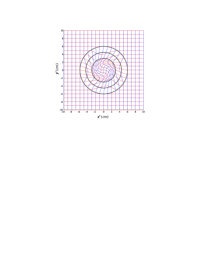
Figure 1: Visualization of the twisted cylindrical concentrator. The mesh grid indicates lines with constant values of $x$ and $y$ plotted in the coordinate system of $x^{\prime}$ and $y^{\prime}$. The radius of the three displayed circles are $R_{1}=3$, $R_{2}=4.5$ and $R_{3}=6$.

The transformation (40) is expressed in cylindrical coordinates. For the calculation of the SHG, however, it is more advantageous to formulate the transformation in Cartesian coordinates in the form $x^{\prime}=x^{\prime}(x,y)$ and $y^{\prime}=y^{\prime}(x,y)$. This is achieved by applying an intermediate transformation $r=\sqrt{x^{2}+y^{2}}$ and $\phi=\arctan(y/x)$ in the unprimed system and an inverse intermediate transformation $x^{\prime}=r^{\prime}\cos\phi^{\prime}$ and $y^{\prime}=r^{\prime}\sin\phi^{\prime}$ in the primed system. With these expressions, the transformation (40) can be re-expressed in Cartesian coordinates by applying the following three subsequent transformations:

$$(x,y)\stackrel{{\scriptstyle f}}{{\longrightarrow}}(r,\phi)\stackrel{{\scriptstyle g}}{{\longrightarrow}}(r^{\prime},\phi^{\prime})\stackrel{{\scriptstyle h}}{{\longrightarrow}}(x^{\prime},y^{\prime}).$$ (43)

According to the chain rule in higher dimension, the Jacobian matrix of a composite function is just the product of the Jacobian matrices of the composed functions, that is

$$A_{f\circ g\circ h}=A_{f}A_{g}A_{h}.$$ (44)

As shown in the appendix, the Jacobian determinants of the intermediate transformations are $|A_{f}|=1/r$ and $|A_{h}|=r^{\prime}$, respectively. Consequently, the Jacobian determinant of the composite is

$$|A_{f\circ g\circ h}|=|A_{f}||A_{g}||A_{h}|=\frac{r^{\prime}}{r}|A_{g}|$$ (45)

with the Jacobian determinant $|A_{g}|$ given in (42). Once the Jacobian matrix and its determinant are known, we can easily transform the fields and material parameters from one coordinate system to the other.

We now intend to calculate the SHG wave generated in the concentrator. For this purpose, we suppose that the material used for the construction of the concentrator exhibits a non-vanishing nonlinear susceptibility. To simplify matters, we further assume that this nonlinearity obeys the phase matching condition for frequency doubling if the fundamental wave and the second harmonic wave are both polarized in the $z$-direction. In our notation, the corresponding tensor component of the nonlinear susceptibility is $a^{\prime}:=4\chi_{0^{\prime}3^{\prime}}^{0^{\prime}3^{\prime}0^{\prime}3^{\prime}}$ (see (18)). For the spatial distribution of $a^{\prime}$, we suppose that the nonlinearity is only present in the inner cylindrical region of the material according to:

$$a^{\prime}(r^{\prime})=\begin{cases}a_{0}&\,0\leq r^{\prime}\leq R_{1}\\[2.84526pt] 0&\,\text{otherwise.}\end{cases}$$ (46)

This could, for example, be realized by doping the center of the concentrator with some nonlinear material.

As fundamental wave we assume an incident monochromatic plane wave that initially propagates along the $x$-axis while the electric field vector is polarized in the $z$-direction. In the physical space of the inhomogeneous material (spanned by primed coordinates), the fundamental wave takes the form:

$$E^{\prime}_{\omega}(x^{\prime},y^{\prime},t)=\mathcal{E}^{\prime}_{\omega}\,e^{i(k_{\omega\,x^{\prime}}^{\prime}x^{\prime}+k_{\omega\,y^{\prime}}^{\prime}y^{\prime}-\omega t)}$$ (47)

where $\mathcal{E}^{\prime}_{\omega}$ denotes the amplitude of the wave and $\bm{k}^{\prime}_{\omega}=(k^{\prime}_{\omega\,x^{\prime}},k^{\prime}_{\omega\,y^{\prime}})$ is the wave vector in the medium. For the second harmonic wave, we represent the electric field by

$$E^{\prime}_{2\omega}(x^{\prime},y^{\prime},t)=\mathcal{E}^{\prime}_{2\omega}(x^{\prime},y^{\prime})\,e^{i(k^{\prime}_{2\omega\,x^{\prime}}x^{\prime}+k^{\prime}_{2\omega\,y^{\prime}}y^{\prime}-2\omega t)}$$ (48)

with the SHG wave vector $\bm{k}^{\prime}_{2\omega}=2\bm{k}^{\prime}_{\omega}$ (phase matched case). In the slowly varying amplitude approximation for the second harmonic wave and the undepleted pump approximation (i.e. $\mathcal{E}^{\prime}_{\omega}$ is constant), the wave equation for the SHG amplitude $\mathcal{E}^{\prime}_{2\omega}(x^{\prime},y^{\prime})$ is given by [31]:

$$\left(k^{\prime}_{2\omega\,x^{\prime}}\frac{\partial}{\partial x^{\prime}}+k^{\prime}_{2\omega\,y^{\prime}}\frac{\partial}{\partial y^{\prime}}\right)\mathcal{E}^{\prime}_{2\omega}(x^{\prime},y^{\prime})=\kappa\mathcal{E}_{\omega}^{{}^{\prime}2}a^{\prime}(x^{\prime},y^{\prime})$$ (49)

with $\kappa=-16\pi i\omega^{2}/c^{2}$. This is a partial differential equation in two dimensions for the second harmonic field amplitude $\mathcal{E}^{\prime}_{2\omega}(x^{\prime},y^{\prime})$ which is very difficult to solve in general. However, the complexity can be significantly reduced if we apply a coordinate transformation to the uniform space (spanned by unprimed coordinates).

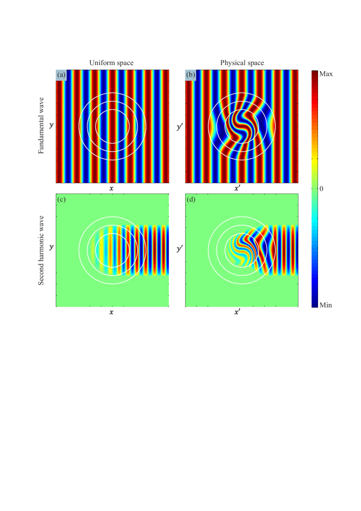
Figure 2: Second harmonic wave generation in a nonlinear cylindrical concentrator. (a) Electric field of the fundamental wave in the uniform space (unprimed system) and (b) in the inhomogeneous, physical space (primed system). (c) Electric field of the second harmonic wave in the unprimed system and (d) in the primed system. The radius of the three displayed circles are $R_{1}=3$, $R_{2}=4.5$ and $R_{3}=6$.

According to (22) and the Jacobian matrix of the transformation given by (44) (with suppressed subscript $f\circ g\circ h$), the $z$-component of the electric field transforms as

$$E^{\prime}_{z^{\prime}}=F_{0^{\prime}3^{\prime}}=A_{0^{\prime}3^{\prime}}^{\mu\;\nu}F_{\mu\nu}=F_{03}=E_{z}$$ (50)

since $t^{\prime}=t$ and $z^{\prime}=z$ implies $A_{0^{\prime}3^{\prime}}^{\mu\;\nu}=\delta_{0}^{\mu}\delta_{3}^{\nu}$. Consequently, the electric fields of both the fundamental and SHG wave remain unchanged under coordinate transformation (but the functional dependence on the underlying coordinate system may be different). Since the unprimed system is homogeneous and isotropic with a refractive index equal to one, the electric field of the fundamental wave in the unprimed system has the form of a uniform plane wave propagating in the $x$-direction:

$$E_{\omega}(x,t)=\mathcal{E}_{\omega}\,e^{i(k_{\omega\,x}x-\omega t)}$$ (51)

with constant amplitude $\mathcal{E}_{\omega}=\mathcal{E}^{\prime}_{\omega}$ and $k_{\omega\,x}=\omega/c$. From this expression, the electric field in the primed coordinate system is readily obtained by expressing $x$ by $x=x(x^{\prime},y^{\prime})$. The real part of the fundamental wave in the primed and unprimed system is plotted in Figs. 2(a) and 2(b), respectively.

Since the fundamental wave propagates straightly along the $x$-direction in the unprimed system and since we assumed phase matching for the SHG process, it follows that the wave vector of the SHG wave is given by $k_{2\omega\,x}=2k_{\omega\,x}=2\omega/c$ and $k_{2\omega\,y}=0$ (on the considered length scale, beam divergence due to diffraction can be neglected). Consequently, the wave equation (49) for the SHG process reduces in the unprimed system to the simple expression

$$\frac{\partial}{\partial x}\mathcal{E}_{2\omega}(x,y)=\frac{\kappa c}{2\omega}\mathcal{E}_{\omega}^{2}a(x,y)$$ (52)

which can be immediately integrated to:

$$\mathcal{E}_{2\omega}(x,y)=\frac{\kappa c}{2\omega}\mathcal{E}_{\omega}^{2}\int_{-\infty}^{x}\!ds\,a(s,y).$$ (53)

The remaining unknown is the nonlinearity $a=4\chi^{0303}_{03}$, i.e. the relevant tensor component for the SHG process in the unprimed system. According to the transformation law derived in (39), the nonlinearity transforms as:

$$a^{\prime} =4\chi^{0^{\prime}3^{\prime}0^{\prime}3^{\prime}}_{0^{\prime}3^{\prime}}=4|A|^{-1}A^{i\;3^{\prime}3^{\prime}}_{3^{\prime}j\,k}\chi^{0j0k}_{0i}=4|A|^{-1}\chi^{0303}_{03}=|A|^{-1}a$$ (54)

since $z^{\prime}=z$ implies that $A_{3^{\prime}j\;k}^{i\;3^{\prime}3^{\prime}}=\delta_{3}^{i}\delta_{j}^{3}\delta_{k}^{3}$. With the determinant $|A|$ given by (45) and (42), the nonlinearity $a^{\prime}$ defined in (46) and the relation between $r$ and $r^{\prime}$ given by (40), we can calculate the nonlinearity in the unprimed system to be:

$$a=\frac{r^{\prime}}{r}|A_{g}|a^{\prime}=\begin{cases}\left(\frac{R_{1}}{R_{2}}\right)^{2}a_{0}&\,0\leq r\leq R_{2}\\[2.84526pt] 0&\,\text{otherwise.}\end{cases}$$ (55)

As expected, the nonlinearity in the unprimed system is reduced by a factor of $(R_{1}/R_{2})^{2}$ compared to the nonlinearity in the primed system (see (46)) because the cylindrical region in which the nonlinear substance is located experiences a space expansion from radius $R_{1}$ to $R_{2}$ if we perform a coordinate transformation from the primed to the unprimed system.

Now we can (even analytically) evaluate the integral (53) for the amplitude $\mathcal{E}_{2\omega}(x,y)$ of the SHG wave. A subsequent multiplication with the propagation phasor yields the SHG wave in the unprimed system in the form:

$$E_{2\omega}(x,y,t)=\mathcal{E}_{2\omega}(x,y)\,e^{2i\omega(x/c-t)}.$$ (56)

By applying the inverse transformation (i.e. expressing $x$ and $y$ by $x=x(x^{\prime},y^{\prime})$ and $y=y(x^{\prime},y^{\prime})$), we finally obtain the SHG wave in the physical space of the primed coordinates. The real part of the resulting SHG field distribution in the two coordinate systems is plotted in Figs. 2(c) and 2(d), respectively.

The proposed twisted nonlinear concentrator is certainly a somewhat constructed example since the exploited uniform space was already presumed in the design of the concentrator. However, the decisive step in the calculation—the straightening of the wave trajectories inside the medium by applying an appropriate coordinate transformation—is in principle always possible in any inhomogeneous media with continuously varying material properties. The proposed technique of simplifying nonlinear processes in inhomogeneous media is therefore not restricted to the presented example, but covers a wide application range.

5 Conclusion

We proposed a theoretical framework for the incorporation of nonlinear effects within the concept of transformation optics (TO). In this context, we derived a general expression for the calculation of linear and nonlinear electromagnetic material parameters under arbitrary coordinate transformations. The transformation law is formulated in a manifestly covariant form that allows the simultaneous treatment of electric, magnetic and magneto-electric cross-coupling terms and is applicable to both temporal and spatial transformations.

As a first application example, we calculated the linear and nonlinear constitutive material relations in a moving medium. As expected from the transformation of electromagnetic fields, the movement of the medium leads to a mixing of the electric and magnetic response, where the obtained expressions for the linear constitutive equations were in agreement with the relations given in the literature. In addition, we showed that the movement of the medium also implies a mixing of the nonlinear material properties which describe cross-coupled nonlinear interactions between the $\bm{E}$- and $\bm{B}$-fields and the medium. This means, for example, that a Pockels medium at rest can display a Faraday effect if the material is moved relative to the observer, and vice versa.

In the final part of the paper we focused on time-independent, spatial coordinate transformations which are of particular interest for the design of nonlinear TO devices. As an illustrative example of such a device, we presented a twisted nonlinear field concentrator and calculated the second harmonic wave that is generated when the concentrator is illuminated by a strong laser field. In this respect, we demonstrated that sophisticated nonlinear phenomena in complex media can take a much simpler form if an appropriate coordinate transformation is applied.

The considerations have shown that the incorporation of nonlinear susceptibilities in the TO approach provides a promising computation method for calculating nonlinear effects in moving or inhomogeneous media and offers new opportunities for the design of novel optical devices with tailored nonlinear properties.

Appendix

Summary of the linear terms in equation (12)

The linear terms in (12) (the free-space contribution and the linear response of the material) can be written as

$$\mathcal{D}_{\mu\nu} =F_{\mu\nu}+4\pi\chi_{\mu\nu}^{\sigma\kappa}F_{\sigma\kappa}$$

$$=\frac{1}{2}\left(F_{\mu\nu}-F_{\nu\mu}\right)+4\pi\chi_{\mu\nu}^{\sigma\kappa}F_{\sigma\kappa}$$

$$=\frac{1}{2}\left(\delta_{\mu\nu}^{\sigma\kappa}-\delta_{\nu\mu}^{\sigma\kappa}\right)F_{\sigma\kappa}+4\pi\chi_{\mu\nu}^{\sigma\kappa}F_{\sigma\kappa}$$

$$=\left(\frac{1}{2}\left(\delta_{\mu\nu}^{\sigma\kappa}-\delta_{\nu\mu}^{\sigma\kappa}\right)+4\pi\chi_{\mu\nu}^{\sigma\kappa}\right)F_{\sigma\kappa}.$$ (57)

And finally, the last line of (12) follows after the re-definition $4\pi\chi_{\mu\nu}^{\sigma\kappa}\,(\text{new}):=\frac{1}{2}\left(\delta_{\mu\nu}^{\sigma\kappa}-\delta_{\nu\mu}^{\sigma\kappa}\right)+4\pi\chi_{\mu\nu}^{\sigma\kappa}$.

Proof of equation (17)

By using the identity

$$F_{ij} =\frac{1}{2}\left(F_{ij}-F_{ji}\right)=\frac{1}{2}\left(\delta_{ij}^{mn}-\delta_{ji}^{mn}\right)F_{mn}$$

$$=\frac{1}{2}g^{k}_{ij}g^{mn}_{k}F_{mn}=-g^{k}_{ij}B_{k}$$ (58)

the components of the electric displacement field are

$$D_{i} =\mathcal{D}_{0i}=4\pi\chi_{0i}^{\sigma\kappa}\,F_{\sigma\kappa}$$

$$=8\pi\chi_{0i}^{0j}F_{0j}+4\pi\chi_{0i}^{mn}F_{mn}$$

$$=8\pi\chi_{0i}^{0j}E_{j}-4\pi g^{j}_{mn}\chi_{0i}^{mn}B_{j}$$ (59)

and, accordingly, the components of the magnetic fields are given by

$$H_{i} =-\frac{1}{2}g_{i}^{mn}\mathcal{D}_{mn}=-2\pi g_{i}^{mn}\chi_{mn}^{\sigma\kappa}\,F_{\sigma\kappa}$$

$$=-4\pi g_{i}^{mn}\chi_{mn}^{0j}F_{0j}-2\pi g_{i}^{mn}\chi_{mn}^{kl}F_{kl}$$

$$=-4\pi g_{i}^{mn}\chi_{mn}^{0j}E_{j}+2\pi g_{i}^{mn}g^{j}_{kl}\chi_{mn}^{kl}B_{j}.$$ (60)

By comparing the expressions of $D_{i}$ and $H_{i}$ with

$$D_{i} =\epsilon_{i}^{j}E_{j}+\xi_{i}^{j}B_{j}$$

$$H_{i} =\zeta_{i}^{j}E_{j}+(\mu^{-1})_{i}^{j}B_{j},$$ (61)

we obtain the relations given in (17).

Number of independent components in $\chi_{\mu\nu}^{\alpha_{1}\beta_{1}\cdots\alpha_{n}\beta_{n}}$

Due to the symmetry properties

$$\chi_{\mu\nu}^{\alpha_{1}\beta_{1}\alpha_{2}\beta_{2}}=-\chi_{\nu\mu}^{\alpha_{1}\beta_{1}\alpha_{2}\beta_{2}}=\chi_{\mu\nu}^{\alpha_{2}\beta_{2}\alpha_{1}\beta_{1}}=-\chi_{\mu\nu}^{\beta_{1}\alpha 1\alpha_{2}\beta_{2}}$$ (62)

(exemplary for $n=2$), there are only 6 independent combinations for each upper index pair $\alpha_{i}\beta_{i}$, e.g. $\alpha_{i}\beta_{i}=01,\,02,\,03,\,12,\,13,\,23$. Furthermore, in the sequence $\alpha_{1}\beta_{1}\cdots\alpha_{n}\beta_{n}$ all $n$ pairs $(\alpha_{i}\beta_{i})$ can be permuted as a whole without changing the value of $\chi_{\mu\nu}^{\alpha_{1}\beta_{1}\cdots\alpha_{n}\beta_{n}}$. Consequently, for fixed lower index pair $\mu\nu$, the number $N$ of independent tensor components is equal to the number of combinations of $n$ labels where each label can take 6 values (with repetition). This number is given by:

$$N(n)=\begin{pmatrix}6+n-1\\ n\end{pmatrix}=\frac{(5+n)!}{5!n!}.$$ (63)

For instance, $N(1)=6$, $N(2)=21$, $N(2)=56$, etc. Finally, we can also vary the lower index pair $\mu\nu$ for which also 6 independent combinations are possible due to the above symmetries. Hence, the total number of independent components of the tensor $\chi_{\mu\nu}^{\alpha_{1}\beta_{1}\cdots\alpha_{n}\beta_{n}}$ is given by $6N(n)$.

Intermediate transformations used in equation (45)

The first intermediate transformation $f$ is given by

$$r =\sqrt{x^{2}+y^{2}}$$

$$\phi =\arctan(y/x)$$ (64)

with the corresponding Jacobian matrix and determinant:

$$A_{f}=\begin{pmatrix}\frac{\partial r}{\partial x}&\frac{\partial r}{\partial y}\\[2.84526pt] \frac{\partial\phi}{\partial x}&\frac{\partial\phi}{\partial y}\end{pmatrix}=\begin{pmatrix}\frac{x}{r}&\frac{y}{r}\\[2.84526pt] -\frac{y}{r^{2}}&\frac{x}{r^{2}}\end{pmatrix},\quad|A_{g}|=\frac{1}{r}.$$ (65)

The inverse intermediate transformation is given by:

$$x^{\prime} =r^{\prime}\cos\phi^{\prime}$$

$$y^{\prime} =r^{\prime}\sin\phi^{\prime}$$ (66)

The corresponding Jacobian matrix and determinant are:

$$A_{h}=\begin{pmatrix}\frac{\partial x^{\prime}}{\partial r^{\prime}}&\frac{\partial x^{\prime}}{\partial\phi^{\prime}}\\[2.84526pt] \frac{\partial y^{\prime}}{\partial r^{\prime}}&\frac{\partial y^{\prime}}{\partial\phi^{\prime}}\end{pmatrix}=\begin{pmatrix}\cos\phi^{\prime}&-r^{\prime}\sin\phi^{\prime}\\[2.84526pt] \sin\phi^{\prime}&r^{\prime}\cos\phi^{\prime}\end{pmatrix},\quad|A_{h}|=r^{\prime}$$ (67)

References

References

- [1] Pendry J B, Schurig D and Smith D R 2006 Science 312 1780–1782
- [2] Leonhardt U 2006 Science 312 1777–1780
- [3] Milton G W, Briane M and Willis J R 2006 New Journal of Physics 8 248 URL http://stacks.iop.org/1367-2630/8/i=10/a=248
- [4] Cummer S A and Schurig D 2007 New Journal of Physics 9 45 URL http://stacks.iop.org/1367-2630/9/i=3/a=045
- [5] Kildishev A V and Shalaev V M 2008 Opt. Lett. 33 43–45 URL http://ol.osa.org/abstract.cfm?URI=ol-33-1-43
- [6] Rahm M, Cummer S A, Schurig D, Pendry J B and Smith D R 2008 Phys. Rev. Lett. 100 063903
- [7] Kundtz N B, Smith D R and Pendry J B 2010 Proc. IEEE PP:99 1–12 ISSN 0018-9219
- [8] Schurig D, Mock J J, Justice B J, Cummer S A, Pendry J B, Starr A F and Smith D R 2006 Science 312 977–980
- [9] Cai W, Chettiar U K, Kildishev A V and Shalaev V M 2007 Nature Photon. 1 224 – 227
- [10] Landy N I, Kundtz N and Smith D R 2010 Phys. Rev. Lett. 105 193902
- [11] Leonhardt U 2011 Nature 471 292 293
- [12] Urzhumov Y A, Kundtz N B, Smith D R and Pendry J B 2011 Journal of Optics 13 024002 URL http://stacks.iop.org/2040-8986/13/i=2/a=024002
- [13] Novitsky A, Qiu C W and Zouhdi S 2009 New Journal of Physics 11 113001 URL http://stacks.iop.org/1367-2630/11/i=11/a=113001
- [14] Kwon D H and Werner D H 2008 Applied Physics Letters 92 013505 (pages 3) URL http://link.aip.org/link/?APL/92/013505/1
- [15] Rahm M, Schurig D, Roberts D A, Cummer S A, Smith D R and Pendry J B 2008 Photonics and Nanostructures-fundamentals and Applications 6 87–95
- [16] Han T, Qiu C and Tang X 2010 Journal of Optics 12 095103 URL http://stacks.iop.org/2040-8986/12/i=9/a=095103
- [17] Nicolet A, Zolla F and Guenneau S 2008 Opt. Lett. 33 1584–1586 URL http://ol.osa.org/abstract.cfm?URI=ol-33-14-1584
- [18] Wang X, Qu S, Xia S, Wang B, Xu Z, Ma H, Wang J, Gu C, Wu X, Lu L and Zhou H 2010 Photonics and Nanostructures - Fundamentals and Applications 8 205–208
- [19] Jiang W X, Chin J Y, Li Z, Cheng Q, Liu R and Cui T J 2008 Phys. Rev. E 77 066607
- [20] Kelley P L 1965 Phys. Rev. Lett. 15(26) 1005–1008 URL http://link.aps.org/doi/10.1103/PhysRevLett.15.1005
- [21] Faust W L and Henry C H 1966 Phys. Rev. Lett. 17(25) 1265–1268 URL http://link.aps.org/doi/10.1103/PhysRevLett.17.1265
- [22] Bloembergen N 1967 35 989–1023 ISSN 00029505 URL http://dx.doi.org/10.1119/1.1973774
- [23] Manassah J T, Baldeck P L and Alfano R R 1988 Opt. Lett. 13 1090–1092 URL http://ol.osa.org/abstract.cfm?URI=ol-13-12-1090
- [24] Shen Y R 1989 Nature 337 519 – 525
- [25] Agrawal G and Olsson N 1989 Quantum Electronics, IEEE Journal of 25 2297 –2306 ISSN 0018-9197
- [26] Macklin J J, Kmetec J D and Gordon C L 1993 Phys. Rev. Lett. 70(6) 766–769 URL http://link.aps.org/doi/10.1103/PhysRevLett.70.766
- [27] Myers L E, Eckardt R C, Fejer M M, Byer R L, Bosenberg W R and Pierce J W 1995 J. Opt. Soc. Am. B 12 2102–2116 URL http://josab.osa.org/abstract.cfm?URI=josab-12-11-2102
- [28] Dubietis A, Butkus R and Piskarskas A 2006 Selected Topics in Quantum Electronics, IEEE Journal of 12 163 – 172 ISSN 1077-260X
- [29] Shen Y R 1976 Rev. Mod. Phys. 48(1) 1–32 URL http://link.aps.org/doi/10.1103/RevModPhys.48.1
- [30] Evans M and Kielich S 1997 Modern Nonlinear Optics (Wiley, New York)
- [31] Boyd R W 2008 Nonlinear Optics (Academic Press, inc.)
- [32] Bergamin L, Alitalo P and Tretyakov S 2011 arXiv:1107.0167v2 [physics.optics]
- [33] Post E J 1997 Formal Structure of Electromagnetics: General Covariance and Electromagnetics (Dover Publications, inc.)
- [34] Thompson R T 2010 Phys. Rev. A 82(5) 053801 URL http://link.aps.org/doi/10.1103/PhysRevA.82.053801
- [35] Thompson R T, Cummer S A and Frauendiener J 2011 Journal of Optics 13 024008 URL http://stacks.iop.org/2040-8986/13/i=2/a=024008
- [36] Rousseaux G 2008 EPL (Europhysics Letters) 84 20002 URL http://stacks.iop.org/0295-5075/84/i=2/a=20002
- [37] Landau L, Lifshitz E and Pitaevskii L 1984 Electrodynamics of Continuous Media (Butterworth-Heinemann, Oxford)
- [38] Cheng D and Kong J A 1968 Proceedings of the IEEE 56 248 – 251 ISSN 0018-9219
- [39] Chen H and Chan C T 2007 90 241105 ISSN 00036951 URL http://dx.doi.org/10.1063/1.2748302