Equilibrium winding angle of a polymer around a bar

Abstract

The winding angle probability distribution of a planar self-avoiding walk has been known exactly since a long time: it has a gaussian shape with a variance growing as $\langle\theta^{2}\rangle\sim\ln L$. For the three-dimensional case of a walk winding around a bar, the same scaling is suggested, based on a first-order epsilon-expansion. We tested this three-dimensional case by means of Monte Carlo simulations up to length $L\approx 25\,000$ and using exact enumeration data for sizes $L\leq 20$. We find that the variance of the winding angle scales as $\langle\theta^{2}\rangle\sim\left(\ln L\right)^{2\alpha}$, with $\alpha=0.75(1)$. The ratio $\gamma=\langle\theta^{4}\rangle/\langle\theta^{2}\rangle^{2}=3.74(5)$ is incompatible with the gaussian value $\gamma=3$, but consistent with the observation that the tail of the probability distribution function $p(\theta)$ is found to decrease slower than a gaussian function. These findings are at odds with the existing first-order $\varepsilon$-expansion results.

1 Introduction

In view of the great importance of DNA in biology and biotechnology, there has been a considerable interest in the past years in the modeling of dynamics and equilibrium properties of DNA molecules [22, 4, 15, 6, 21, 8, 24, 5, 14, 2]. From the perspective of statistical physics, DNA is an interesting system as it shows a broad range of phenomena such as phase transitions in response to temperature changes and to the application of mechanical forces. A paradigmatic example is that of the melting transition, i.e. the separation of the two strands of the helix induced by a temperature change, which has been the object of considerable attention by the scientific community [22, 4, 15, 6, 21]. Also the melting dynamics, and in particular the openings of bubbles, has been the topic of various studies [18, 16, 3]. A new aspect which shows up prominently in the dynamics, while being of less importance in equilibrium, is the helical nature of the double-stranded DNA, which lead to models of DNA molecules which approximately include helical degrees of freedom [8, 24, 5, 14]. Also, in a recent simulation study involving two of us [2], the scaling relation between the unwinding time $\tau_{u}$ of a double-helical structure, as a function of its length $L$, has been studied, with the result $\tau_{u}\sim L^{2.58\pm 0.02}$. A theoretical understanding of this scaling is still missing.

A system closely related to the unwinding of a double-helical structure, is the unwinding of a single polymer initially wound around a fixed bar. The advantage of this latter system is that it has a cleanly defined reaction coordinate: the winding angle of the free end. While it is our ultimate goal to understand fully the dynamics of unwinding, the topic of the current research is restricted to identify the equilibrium properties of a single polymer wound around a bar, thereby providing a solid basis for further research.

Further motivation behind our study, is that there has been quite some recent interest in the study of topological properties of long flexible polymers, inspired by biology, in the context of chromosomal segregation (see e.g. Ref. [19]). The scaling behavior of the probability distribution function of linking numbers of two closed polymer rings reveals some interesting properties which could explain segregation of chromatide domains [19]. The winding angle distribution of a polymer attached to a bar is an analog of the linking number, so it is natural to ask whether the results discussed here could be extended to other topological invariants for closed curves.

2 Winding angle distributions

The study of winding properties of random and self-avoiding walks has a long history which dates back to more than half a century ago [27]. These properties are relevant for many applications in different domains of statistical physics [11, 26, 10, 13, 9, 23]. In a few simple cases the probability distribution function (pdf) of winding angles can be computed exactly. For instance, the pdf of a planar random walk winding around a circle of finite radius is [25]

$$\lim_{L\to\infty}p\left(x=\frac{2\theta}{\ln L}\right)=\frac{\pi}{4}\frac{1}{\cosh^{2}(\pi x/2)},$$ (1)

where $\theta$ is the winding angle and $L$ the length of the walk. These quantities appear in the pdf as a single scaling variable $x=2\theta/\ln L$.

Planar self-avoiding walks were studied first by Fisher et al. [11]. On the basis of scaling arguments and numerical results they suggested that the distribution of winding angles is gaussian with a variance growing as $\langle\theta^{2}\rangle\sim\ln L$ (as opposed to that of planar random walks in which $\langle\theta^{2}\rangle\sim(\ln L)^{2}$, see Eq. (1)). These findings were corroborated by an exact distribution [10]

$$\lim_{L\to\infty}p\left(x=\frac{\theta}{2\sqrt{\ln L}}\right)=\frac{1}{\sqrt{\pi}}e^{-x^{2}},$$ (2)

obtained some years later by conformal invariance techniques.

The winding angle distribution of several other polymer systems were considered, as for instance two-dimensional polymers with orientation-dependent interactions [23]. The phase diagram of these polymers contains different phases, e.g. spiral collapsed, normal collapsed and swollen, separated by a theta point. The winding angle distribution turns out to be universal [23]. It is gaussian with a variance $\langle\theta^{2}\rangle=C\ln L$, where the coefficient $C$ takes different values in different phases. The gaussian behavior is therefore a robust feature for self-avoiding walks in two dimensions.

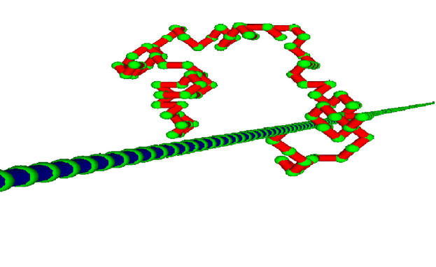
Figure 1: Snapshot of an equilibrium Monte Carlo simulation of a three-dimensional polymer attached to an infinitely long bar. The polymer is self-avoiding and has excluded-volume interactions with the bar.

No exact distribution is known in the case of a polymer attached by one end to a rigid bar, which is the case studied in this paper (see Fig. 1). Using renormalization group techniques, in 1988, Rudnick and Hu [26] considered a self-avoiding walk in $4-\varepsilon$ dimensions whose path wraps around a surface of dimension $2-\varepsilon$. The probability distribution for a winding angle $\theta$ of a polymer of length $L$, at first order in $\varepsilon$, is [26]

$$p(\theta,L,\epsilon)\propto\exp\left(-\theta^{2}\varepsilon/8\ln L\right),$$ (3)

which surprisingly matches the exact form of a planar self-avoiding walk, given in Eq. (2), by simply setting $\varepsilon=2$. The authors of Ref. [26] also performed numerical calculations of the variance $\langle\theta^{2}\rangle$ for self-avoiding walks of length $L\leq 800$. Due to the limited computing power available at that time, only a pre-asymptotic regime could be investigated, which showed a scaling consistent with that of random walks: $\langle\theta^{2}\rangle\sim(\ln L)^{2}$.

Another interesting class of systems is three-dimensional directed walks winding around a line [9], which model the behavior of flux lines in high-$T_{c}$ superconductors. When projected on the plane perpendicular to the line, the winding problem reduces to that of a two-dimensional random walk winding around a center. The winding angle distribution follows again an exponential decay (as for Eq. (1)), with a decay constant depending on the type of boundary conditions [9]. The distribution is however a gaussian in the presence of random impurities in the bulk [9] with the same scaling variable as in Eq. (2). The pinning effect of the impurities makes the walks meander in the direction away from the line, with an excursion size growing as $\sim l^{0.62}$ for a path of length $l$. This behavior is close to that of three-dimensional self-avoiding walks ($\sim l^{\nu}$ with $\nu\approx 0.588$), which may suggest that the winding angle distribution of self-avoiding walks around a bar would be gaussian. This would also be in agreement with the $\varepsilon$-expansion distribution (Eq. (3)), when setting $\varepsilon=1$. We will, however, show that the winding angle distribution for a self-avoiding walk around a bar does not follow gaussian behavior. In addition the variance $\langle\theta^{2}\rangle$ turns out to scale with a non-trivial power of $\ln L$.

3 The Model

The numerical results presented in this paper are obtained by Monte Carlo simulations of lattice polymers up to $L\approx 25\,000$ on a face-centered-cubic lattice and by exact enumerations of short walks ($L\leq 20$) on a cubic lattice. In both cases one end of the polymer is attached to the bar, while the other is free. In the exact enumeration study all the possible configurations of a polymer attached at one end to a bar on a simple cubic lattice were generated using a backtracking method, and the averaged squared winding angle was computed.

In the Monte Carlo simulations we performed equilibrium sampling using two types of updates: (1) local moves, such as corner flips and end-monomer flips and (2) global moves, involving the rotation of a whole branch of the polymer from a selected point via the pivot algorithm (see [17] for a detailed study of this algorithm). This algorithm is very efficient because of the small autocorrelation time. Recently it was applied to the computation of the growth exponent $\nu$ for very long polymers [7]. One monomer is chosen randomly as the pivot point and a random operation of symmetry allowed by the lattice (rotation or reflection) is applied to the branch of the polymer not attached to the bar. This attempt is accepted if it satisfies the self-avoidance.

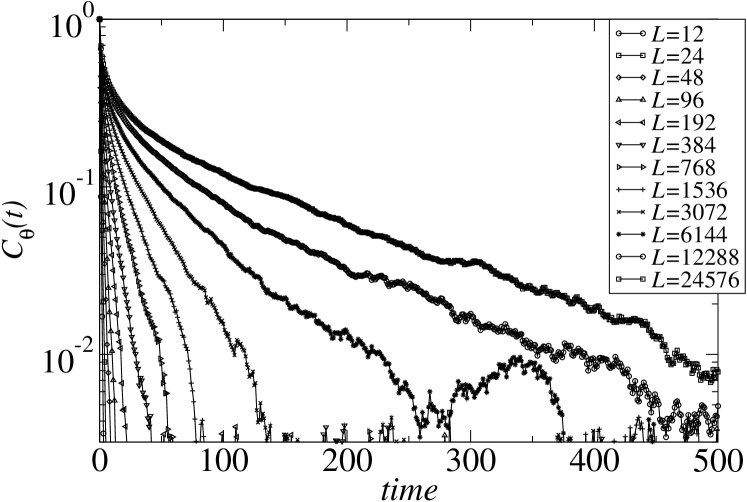
Figure 2: Autocorrelation function of the winding angle calculated for sizes $L=6\cdot 2^{n}$ with $n\in[1;8]$ (from bottom to top). A unit of time corresponds to $L$ attempts with corner flips and 15 attempted pivots. The correlation time is estimated through the integration of these curves [20].

The acceptance ratio $R$ (the ratio of accepted moves over the total number of attempts) of the pivot algorithm scales as $R\propto L^{-p}$ where $p\approx 0.1918(13)$ in two dimensions and $p\approx 0.1069(9)$ in three dimensions [17]. Our estimates for $R$ compare well with those of [17], but are however slightly smaller due to collisions with the bar. For the range of sizes investigated in this article, the acceptance ratio varies between $R\approx 0.6$ ($L\approx 100$) and $R\approx 0.33$ ($L\approx 25\,000$). In the following, one unit of time consists of 15 attempted pivots moves, on average corresponding to 5 accepted pivot moves for the biggest sizes, and $L$ attempted corner flips. Since the structure of the FCC lattice allows a winding over an angle of $2\pi$ within 6 links, the maximum winding angle is $2\pi L/6$. We choose the polymer length as a multiple of 6: $L=6\cdot 2^{n}$ with $2\leq n\leq 8$ i.e. up to $L=24576$. The correlation time $\tau$ is estimated through the autocorrelation function $C_{\theta}(t)$ of the winding angle $\theta$. It is defined as

$$C_{\theta}(t)=\frac{\langle\theta(0)\theta(t)\rangle-\langle\theta\rangle^{2}}{\langle\theta^{2}\rangle-\langle\theta\rangle^{2}},$$ (4)

where the symbol $\langle\cdots\rangle$ indicates the equilibrium average. The results are shown in Figure 2. From the data we estimate that $\tau\approx 80$ for $L=24576$. We performed a thermalization during at least $20\tau$, followed by samplings separated by at least $2\tau$. We considered polymers of lengths from $L=12$ to $L=24576$, each time separated by a factor 2. Since the samplings can be considered as independent, the fluctuations are estimated using the central limit theorem [20].

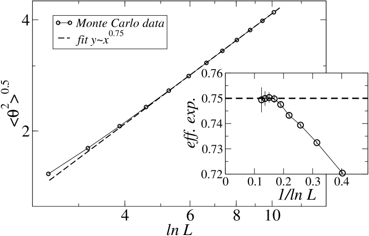
Figure 3: Double-logarithmic plot of $\sqrt{\langle\theta^{2}\rangle}$ vs. $\ln L$ for $L=12$ up to $24576$ with steps of factors of $2$. The data for $L>400$ are described within error bars by a power-law $\sqrt{\langle\theta^{2}\rangle}\propto(\ln L)^{\alpha}$ with $\alpha=0.75(1)$. Inset: effective exponent as a function of $1/\ln L$.

4 Results

4.1 Analysis of $\langle\theta^{2}\rangle$

Figure 3 shows a double-logarithmic plot of $\sqrt{\langle\theta^{2}\rangle}$ as a function of $\ln L$, calculated up to a size $L_{\rm max}=24\,576$. Averages were performed over $2\cdot 10^{6}$ and $10^{6}$ independent configurations, respectively, for sizes ranging between $L=12$ and $1536$, and between $L=3072$ and $24\,576$. The dashed line represents the best fit to the data, which implies a scaling of the type $\sqrt{\langle\theta^{2}\rangle}\sim(\ln L)^{\alpha}$ with $\alpha\approx 0.75$. The inset in Fig. 3 shows the effective exponent which was computed from the slope of the data in the interval $[L,L_{\rm max}]$ for increasing $L$. The effective exponent is plotted as a function of $1/\ln L$ and shows a convergence to $\alpha=0.75(1)$.

A second analysis was performed on polymers with lengths $L=10^{2}$, $10^{3}$ and $10^{4}$, each averaged over $10^{6}$ independent configurations. We computed the winding angle as a function of the monomer index $i$, which is shown in Fig. 4. This analysis is done on a large number of data points as $1\leq i\leq L$ and yields $\sqrt{\langle\theta^{2}\rangle}\sim(\ln i)^{\alpha}$ with $\alpha\approx 0.75$, again consistent with the previous estimate ($i=1$ is the monomer attached to the bar, while $i=L$ is the free end monomer). The effective exponent, calculated as above and plotted as a function of $1/\ln i$, is shown in the inset of Fig. 4. Starting from small $i$ (right side of the graph), the data quickly reach a rather constant value, while the effective exponent decreases for $i\to L$, due to an abrupt change of slope close to the free end of the polymer. This behavior is due to end effects and was discarded from the analysis. We estimated the exponent from the constant plateau value (dashed line), yielding $\alpha=0.75(2)$. Note that for the longest polymer $L=10^{4}$ the region with a constant $\alpha_{\rm eff}$ is considerably broader.

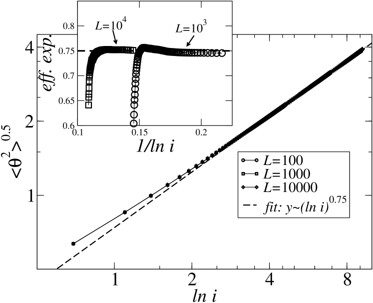
Figure 4: Plot of $\sqrt{\langle\theta^{2}\rangle}$ vs. $\ln i$ (the monomer index) for three polymers of lengths $L=10^{2}$, $10^{3}$ and $10^{4}$. Inset: the effective exponent for the two largest sizes. Disregarding the strong devations close to the end monomer $i=L$, we estimate $\alpha=0.75(2)$ (dashed line).

Figure 5 shows a plot of the average winding angle of the $i$-th monomer as a function of the mean square distance $\langle r_{i}^{2}\rangle$ from the monomer $i=1$, which is attached to the bar. Since $r_{i}\sim i^{\nu}$ we expect $\sqrt{\langle\theta^{2}\rangle}\sim(\ln\langle r_{i}^{2}\rangle)^{\alpha}$. The best fit of the data in the log-log plot yields a value $\alpha\approx 0.8$ (dashed line), which is slightly higher than the previous estimates. The inset of Fig. 5 shows the plots of the integrated effective exponents plotted as function of $1/\ln\langle r_{i}^{2}\rangle$. As was the case in Fig. 4, we notice a divergence of the effective exponents for $i\to L$ due to end effects. We notice also strong finite size effects since corrections to scaling can arise from both $\langle r_{i}^{2}\rangle$ and $\sqrt{\langle\theta^{2}\rangle}$. An accurate estimate of $\alpha$ is more difficult from these data. However, when increasing the polymer length, the effective exponent decreases (ignoring the end behavior), suggesting as upper bound $\alpha<0.8$.

Summarizing, the analysis of Monte Carlo data yield a consistent value of $\alpha\approx 0.75(1)$, at least for the first two quantities analyzed. We note that the computed value of $\alpha$ is between the two-dimensional random walk case $\alpha=1$ (Eq. 1) and the two-dimensional self-avoiding walk case $\alpha=1/2$ (Eq. 2). It can be interpreted as follow. Projecting the polymer configuration onto a plane perpendicular to the bar one obtains a two-dimensional projection where the walk has some overlaps, but the three-dimensional self-avoidance constraints reduces these overlaps compared to those of a full planar random walk.

Figure 5: Logarithmic plot of $\sqrt{\langle\theta^{2}\rangle}$ vs. $\ln\langle r^{2}_{i}\rangle$ where $\langle r^{2}_{i}\rangle$ is the mean square distance of the monomer $i$ from the monomer attached to the bar. Shown are the data for polymers of lengths $L=10^{2}$, $10^{3}$ and $10^{4}$. Inset: plot of the effective exponents for the three sizes. Due to strong finite-size effects, the exponent is not converging for the different sizes. We can only conclude an upper bound $\alpha<0.8$.

To corroborate these finding we also performed exact enumerations of a self-avoiding walk winding around a bar on the cubic lattice. As the number of walks grows exponentially in $L$ the calculations were restricted to $L\leq 20$. The table 1 gives the total number of walks, the average squared end-to-end distance $\langle r^{2}\rangle$, the average squared winding angle $\langle\theta^{2}\rangle$ and the ratio $\langle\theta^{4}\rangle/\langle\theta^{2}\rangle^{2}$. In Figure 6 we show a log-log plot of $\sqrt{\langle\theta^{2}\rangle}$ as a function of $\ln L$. These data are consistent with those obtained from the Monte Carlo analysis, namely of a power-law behavior $\sqrt{\langle\theta^{2}\rangle}\sim(\ln L)^{\alpha}$ with $\alpha\approx 0.75$. The calculation of the effective exponent is plotted as a function of $1/\ln L$ in the inset of Fig. 6. As seen from the data the effective exponent is linearly related to $1/\ln L$. A linear extrapolation for infinite sizes using $1/\ln L$ as scaling variable gives $\alpha\approx 0.78$, which is close to the estimate from Monte Carlo simulations. Strong oscillations for odd-even sizes do not allow the use of more refined extrapolation methods such as the BST algorithm [12].

Table 1: Exact enumeration results for a self-avoiding walk on a cubic lattice, which is attached to a bar. For sizes ranging from 2 to 20 steps. Measured are the number of walks, their average squared end-to end distance $\langle r^{2}\rangle$, the average squared winding angle $\langle\theta^{2}\rangle$, and the ratio $\langle\theta^{4}\rangle/\langle\theta^{2}\rangle^{2}$.

Size	Num. walks	$\langle r^{2}\rangle$	$\langle\theta^{2}\rangle$	$\langle\theta^{4}\rangle/\langle\theta^{2}\rangle^{2}$
2	20	2.400000	0.246740	2.50001
3	92	4.130435	0.573089	2.43716
4	444	5.801802	0.801767	2.69437
5	2076	7.736031	1.008331	2.90674
6	9860	9.619473	1.177011	3.09368
7	46356	11.654241	1.338818	3.18679
8	219316	13.667001	1.475501	3.28308
9	1031836	15.795530	1.608453	3.33777
10	4871212	17.908542	1.725029	3.39814
11	22917588	20.115627	1.837856	3.42916
12	108046716	22.311513	1.939638	3.47006
13	508228828	24.585907	2.037864	3.48878
14	2393946452	26.852009	2.128326	3.51787
15	11257861180	29.185833	2.215473	3.53001
16	52994270612	31.513181	2.296973	3.55151
17	249151623836	33.900291	2.375421	3.55988
18	1172249039916	36.282137	2.449638	3.57625
19	5510044713020	38.717590	2.521054	3.58235
20	25914234060972	41.148633	2.589254	3.59503

Figure 6: Double-logarithmic plot of $\sqrt{\langle\theta^{2}\rangle}$ vs. $\ln L$ from the exact enumeration data. Inset: plot of the effective exponent as a function of $1/\ln L$. A linear extrapolation of the effective exponent using a $1/\ln L$ variable gives $\alpha\approx 0.78$, which is close to the estimate from Monte Carlo data.

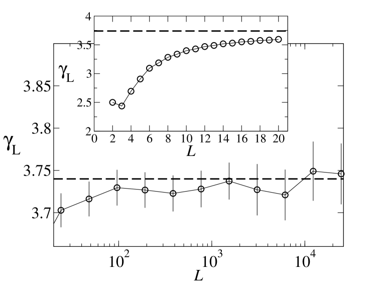
Figure 7: Dependence of the ratio $\frac{\langle\theta^{4}\rangle}{{\langle\theta^{2}\rangle}^{2}}$ with respect to the size. Main graph: we observe fluctuations around $3.74(5)$ but no shift toward the value $3$ of the gaussian distribution. For convenience of the reader, the horizontal axis is logarithmic. Insert: data from exact enumeration of the simple cubic lattice. The dotted line indicates the value obtained in the main graph.

4.2 The probability distribution function (pdf)

We consider now the pdf of winding angles $p(\theta,L)$. Equivalently, this is related to the free energy as a function of winding angle, using the relation

$$\beta F=-\ln\left(p(\theta,L)/p(0,L)\right).$$ (5)

A direct evidence of the non-gaussian behavior of this distribution is provided by Monte Carlo simulations with the same parameters as the previous subsection. The main frame of Fig. 7 shows the value of the ratio

$$\gamma_{L}=\frac{\langle\theta^{4}\rangle}{\langle\theta^{2}\rangle^{2}}$$ (6)

plotted for differents sizes. We obtain the estimate $\gamma=3.74(5)$, which is a value well above the expectation for a gaussian distribution ($\gamma=3$ for a gaussian pdf). The exact enumeration data reported in the last column of Table 1 for different polymer lengths are shown in the inset of Fig. 7. They display a convergence in good agreement with the value obtained from Monte Carlo simulation (dashed line).

The full plot of the winding angle distribution function is shown in Fig. 8 for Monte Carlo simulations. The binning of the winding angles is done with intervals of $\approx 0.5$ rad. The data for the different lengths collapse very well onto a single curve when the scaling variable $x=\theta/(\ln L)^{0.75}$ is used, a value which confirms the exponent obtained from the analysis of the variance of the winding angle. The inset of Fig. 8 shows a log-log plot of $p(0,L)$ as a function of $\ln L$ confirming again the scaling exponent $\alpha\approx 0.75$. The pdf is thus described by a scaling form of the type

$$p(\theta,L)=\frac{Cst.}{(\ln L)^{\alpha}}f\left(\frac{\theta}{(\ln L)^{\alpha}}\right)$$ (7)

where $f(x)$ is a scaling function. The dashed line in Fig. 8 shows a parabolic fit of the data. It indicates that the tail of the distribution decays slower than that of a gaussian distribution.

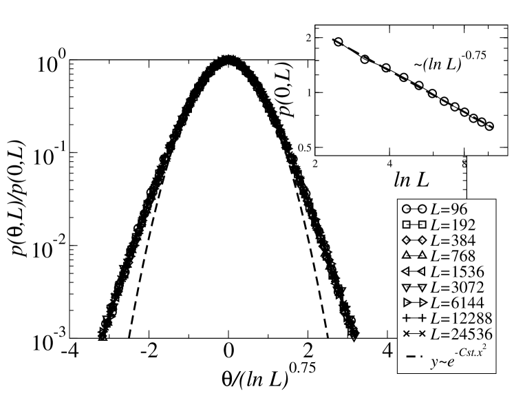
Figure 8: Histogram of the winding number of the polymer around the bar. The probability is normalized and plotted vs. $(\ln L)^{0.75}$. The data display a scaling behavior, confirming the power law found above. The dotted line is a gaussian fit which clearly does not fit the data as $\theta$ increases. Insert : $p(0,L)$ is plotted vs. $\ln L$ and behaves as $p(0,L)\sim(\ln L)^{-0.75}$.

In order to sample the tail of the distribution with a sufficient statistical accuracy, i.e., beyond the data shown in Fig. 8, we have used a reweighting technique. A weight $\exp(A(\theta_{a}-\theta_{b}))$ was added in the acceptance probability of each Monte Carlo move. The angles $\theta_{b}$ and $\theta_{a}$ are respectively the angles before and after the Monte Carlo trial move and $A$ is a positive constant. This favors large winding angles depending on the value of the constant $A$. The distributions obtained are then multiplied by $\exp(-A\theta)$ to retrieve unbiased results. The results are shown in Fig. 9 for lattices sizes ranging between $L=96$ and 1536 by steps of a factor of two. The results are averaged over $10^{7}$ configurations, i.e., five times more than the histogram of Fig. 8, so we restricted ourselves to smaller sizes compared to those of Fig. 8. We have chosen the value $A=0.45$ for all sizes. For the two smallest sizes, finite-size effects occur for large winding. However, other than that, the data display a nice scaling collapse until $p(\theta)/p(0)\approx 10^{-10}$. These results confirm the scaling behavior observed at smaller winding angles on Fig.8.

Figure 9: Histogram of the winding angle of the polymer around the bar. The probability is estimated through biased sampling, such that the region of large winding and low probability is visited. The two smallest sizes start to display finite-size effects for large winding angles. However, the three largest sizes show a good collapse with the scaling variable $\theta/(\ln L)^{0.75}$.

Figure 10 shows the same data as in Fig. 9, this time showing the free energy as a function of the scaling variable $\theta/(\ln L)^{\alpha}$ with $\alpha=0.75$, in a double-logarithmic plot. For small winding angles the free energy increases quadratically in $\theta$, which is the harmonic response to small winding. At higher $\theta$’s, the shape of the free-energy curve changes and follows a different behavior, which corresponds to the deviation from the gaussian shape observed in the pdf.

Figure 10: Free energy plotted as function of the scaling variable $x=\theta/(\ln L)^{\alpha}$ for polymers of various lengths. This quantity shows a crossover from $\sim x^{2}$ behavior at small $x$ (dashed line) towards a different regime at higher winding. The fit of the data at high winding yields $\sim x^{1.3}$ (dashed-dotted line).

Although the range of $\theta$ one can analyze with the reweighting method described above is somewhat limited, the data suggest a possible crossover from the gaussian behavior $F\sim x^{2}$ at small $x=\theta/(\ln L)^{\alpha}$ i.e. small $\theta$, to a different power-law. A power-law fit in the region of high winding numbers yields a behavior $F\sim x^{1.3}$. This behavior is reminiscent of the scaling of the free energy for the gaussian linking number of two tethered rings [19]. The linking number is a topological invariant and indicates the degree of entanglement of two polymer rings. This quantity roughly represents the number of times that each rings winds around the other, and can thus be considered an analogous of the winding angle $\theta$ of a polymer wound around a bar.

For random walks, the free energy as a function of the linking number $Ca$ was found to scale as [19] $F\sim Ca^{2}$ for small $Ca$ and as $F\sim Ca^{4/3}$ at stronger $Ca$, from simulation data and analytical arguments. It is however not yet clear whether this analogy holds for the winding angle distribution, as for self-avoiding tethered rings the free energy is linear in the linking number $F\sim Ca$, suggesting phase separation.

We propose the following arguments to justify the non-gaussianity of the curves. As noted before, the maximal winding number that can be achieved with a polymer of length $L$ is $\theta_{max}=2\pi L/6$. An upper limit to the range in free energy is given by $\Delta F\leq\beta^{-1}\log(Z_{L})$ where $Z_{L}$ is the total number of states accessible to the polymer. Since the set of random-walk configurations is a superset of the set of self-avoiding-walk configurations wrapped around a bar, it follows that $Z_{L}<\mu^{L}$ with $\mu=6$ for a cubic, and $\mu=12$ for a fcc lattice, and thus it follows that $\log(Z_{L})\leq\mu L$. Consequently, the free energy of the the maximally wound state can at most increase linearly with $L$, and certainly not quadratically. Hence, the existence of a maximally wound state with $\theta\sim L$ together with the maximal range in free energy of $\sim L/\beta$ already provides proof of nongaussian behavior of the pdf at large winding. (Note that for two-dimensional self-avoiding walks, the same argument does not exclude a gaussian distribution, as the maximal winding angle is then $\theta_{max}\sim\sqrt{L}$).

4.3 The polymer shape

We consider next the equilibrium shape of the polymer wound around the bar at some fixed winding angle $\theta$. We use cylindrical coordinates where the bar is the reference axis and the origin is the point of attachment of the polymer. $R_{i}$ is the radial coordinate where $i$ labels the monomers, starting from the monomer attached to the bar. $z_{i}$ is the coordinate in the direction parallel to the bar, and $\omega_{i}$ is the winding angle of the monomer $i$ along the polymer. The total winding angle is given by $\omega_{L}=\theta$.

In order to sample configurations with high winding we have performed reweighted simulations as explained in the previous subsection, using the parameter $A=0.45$. In this way a broad range of values of $\theta$ were generated in the course of the simulation. Each time a configuration with a winding angle equal to $\theta_{n}=n\pi/2$ with $0\leq n\leq 14$ was generated the cylindrical coordinates $(R_{i},\omega_{i},z_{i})$ were stored. In this way the averaged shape was computed for some selected winding angles $\theta_{n}$ (in practice we sampled over all configurations with winding in the interval $[\theta_{n}-0.01,\theta_{n}+0.01]$).

The range of values of $\theta$ analyzed spans completely the region shown in Fig.9, i.e., the region containing the equilibrium configurations with a significant probability. Figure 11 (top) plots the behavior of $z_{i}^{2}$ vs $i$ (main graph) and of $R_{i}$ vs $i$ (insert) for different total winding angles $\theta_{n}$. For all values of $\theta_{n}$ investigated, the data follow rather well the self-avoiding walk scaling $z_{i}^{2}\sim i^{2\nu}$, where $\nu=0.588$ is the Flory exponent [28]. In addition, the data corresponding to different winding angles $\theta$ overlap, showing that the distribution of the monomers in the direction parallel to the bar is weakly influenced by the total winding angle. The inset of Fig. 11 (top) shows the behavior of $R_{i}^{2}$ vs. $i$. In this case there is a stronger dependence on the winding angle. For a given $i$, the distance from the bar $R_{i}$ decreases at higher winding angles, as expected. For the smallest winding (top curve), the data follow quite well the scaling $R_{i}^{2}\sim i^{2\nu}$. For higher winding angles $R_{i}$ keeps increasing monotonically with $i$, but the data show a kink close to the polymer end.

Figure 11 (bottom) plots $\omega^{2}$ vs. $\ln R^{2}$ for different total winding angles $\theta$, obtained as discussed above. The data are plotted on a log-log scale. The lowest curve corresponds to the smallest winding angle analyzed ($\theta=0$). We note that the behavior is non-monotonic, implying that inner monomers can have a higher winding, compared to the end monomer. For higher total winding angles, the curves are monotonic. The values of $\theta$ for which the crossover between non-monotonic to monotonic scaling occurs, corresponds approximately to the crossover between quadratic to non-quadratic response in the free energy discussed in the previous subsection. A straight line in the plot of Fig. 11 (bottom) would correspond to a shape described by a stretched exponential

$$R(\omega)\sim e^{\Gamma\omega^{\gamma}}$$ (8)

Although for a few intermediate winding angles the lines appear to be rather straight in the graphs, it is difficult to capture the shape with a simple analytical form. However, these shapes could be compared with those obtained during unwinding dynamics [2].

Figure 11: Configuration of a polymer of size $L=1536$ for different winding angles $\theta$. Top: the coordinate $z_{i}$ (main graph) and $R_{i}^{2}$ (inset) versus the monomer index $i$. Bottom: the two relevant coordinates of the system: $\omega^{2}_{i}$ versus $\ln R^{2}_{i}$. For intermediate values of $\theta$, they display a power law relation.

5 Conclusion and future work

In this paper we have investigated the equilibrium behavior of a polymer wound around an infinitely long bar. The polymer is self-avoiding and it has excluded volume interactions with the bar as well. The main result of the paper is that the pdf is described by a scaling variable of the type $\theta/(\ln L)^{\alpha}$, where $\alpha\approx 0.75$. The fact that scaling involves the logarithm of the polymer length is not surprising, as this is also found in the case of two-dimensional self-avoiding and random walks. The exponent $\alpha$ in those two cases is however different with $\alpha=1$ for planar random walks [25] and $\alpha=1/2$ for self-avoiding walks [10]. The case of a three-dimensional polymer appears to be intermediate between the two. The presence of a logarithm is responsible for slow asymptotic convergence and some care has to be taken in this case. Our analysis, however, involves very long polymers with $L\approx 25\,000$, and thanks to a reweighting technique, explores high winding numbers, i.e., low-probability regions of the distribution. In addition several different quantities have been analyzed and all confirm $\alpha\approx 0.75$. The same holds for exact enumeration results.

The pdf itself appears to deviate from a gaussian behavior. The ratio $\gamma=\langle\theta^{4}\rangle/\langle\theta^{2}\rangle^{2}=3.74(5)$ differs from the gaussian value $\gamma=3$. This is best characterized by the scaling of the free energy which crosses over from $F\sim x^{2}$ at small $x=\theta/(\ln L)^{\alpha}$, towards a behavior characterized by a different power-law $F\sim x^{1.3}$, although in a small range of values of $x$.

More analytic insights in these problems are lacking at the moment. These are restricted to a first-order $\varepsilon$-expansion around four dimensions [26]. These results suggest a scaling behavior with $\alpha=1/2$ also in three dimensions which is at odds with our present numerical findings.

Our future work will proceed along various lines. First, to connect our work more directly with DNA melting, we intend to introduce an attractive interaction between the polymer and the bar, mimicking the hybridization between the two DNA-strands. This interaction will initially be homogeneous, but later might have a random component to capture the difference between the binding strengths of AT and CG bonds. How such interactions influence the equilibirum statistics of winding, is an open issue. Secondly, we want to combine the results presented here with earlier work involving some of us on the unwinding dynamics [2], which is still an open issue.

References

References

- [1] M. Baiesi, G. T. Barkema, and E. Carlon. Elastic lattice polymers. Phys. Rev. E, 81(6):061801, 2010.
- [2] M. Baiesi, G. T. Barkema, E. Carlon, and D. Panja. Unwinding dynamics of double-stranded polymers. J. Chem. Phys., 133:154907, 2010.
- [3] M. Baiesi and R. Livi. Multiple time scales in a model for DNA denaturation dynamics. J. Phys. A: Math. Theor., 42:082003, 2009.
- [4] M. Barbi, S. Cocco, M. Peyrard, and S. Ruffo. A twist opening model for DNA. Journal of Biological Physics, 24:97–114, 1999.
- [5] M. Barbi, S. Lepri, M. Peyrard, and N. Theodorakopoulos. Thermal denaturation of an helicoidal DNA model. Phys. Rev. E, 68:061909, 2003.
- [6] E. Carlon, E. Orlandini, and A. L. Stella. Roles of stiffness and excluded volume in DNA denaturation. Phys. Rev. Lett., 88:198101, 2002.
- [7] N. Clisby. Accurate estimate of the critical exponent for self-avoiding walks via a fast implementation of the pivot algorithm. Phys. Rev. Lett., 104:055702, 2010.
- [8] S. Cocco and R. Monasson. Statistical mechanics of torque induced denaturation of DNA. Phys. Rev. Lett., 83:5178, 1999.
- [9] B. Drossel and M. Kardar. Winding angle distributions for random walks and flux lines. Phys. Rev. E, 53:5861–5871, 1996.
- [10] B. Duplantier and H. Saleur. Winding-angle distributions of two-dimensional self-avoiding walks from conformal invariance. Phys. Rev. Lett., 60:2343–2346, 1988.
- [11] M. E. Fisher, V. Privman, and S. Redner. The winding angle of planar self-avoiding walks. J. Phys. A: Math. Gen., 17:L569, 1984.
- [12] M. Henkel and G. Schutz. Finite-lattice extrapolation algorithms. J. Phys. A: Math. Gen., 21(11):2617–2633, 1988.
- [13] B. Houchmandzadeh, J. Lajzerowicz, and M. Vallade. Influence of chiral interactions on the winding and localization of a polymer chain on a rigid rod molecule. J. Phys. I France, 2:1881–1888, 1992.
- [14] A. Kabakçıoğlu, E. Orlandini, and D. Mukamel. Supercoil formation in dna denaturation. Phys. Rev. E, 80:010903, 2009.
- [15] Y. Kafri, D. Mukamel, and L. Peliti. Why is the DNA denaturation transition first order? Phys. Rev. Lett., 85:4988, 2000.
- [16] H. Kunz, R. Livi, and A. Süto. The structure factor and dynamics of the helix-coil transition. J. Stat. Mech.: Theory and Exp., 2007(06):P06004, 2007.
- [17] N. Madras and A. D. Sokal. The pivot algorithm: A highly efficient monte carlo method for the self-avoiding walk. J. Stat. Phys., 50:109–186, 1988.
- [18] D. Marenduzzo, S. M. Bhattacharjee, A. Maritan, E. Orlandini, and F. Seno. Dynamical scaling of the DNA unzipping transition. Phys. Rev. Lett., 88:028102, 2001.
- [19] J. F. Marko. Linking topology of tethered polymer rings with applications to chromosome segregation and estimation of the knotting length. Phys. Rev. E, 79:051905, 2009.
- [20] M. E. J. Newman and G. T. Barkema. Monte Carlo Methods in Statistical Physics. Oxford University Press, New York, 1999.
- [21] M. Peyrard. Biophysics: Melting the double helix. Nature Phys., 2:13, 2006.
- [22] M. Peyrard and A. R. Bishop. Statistical mechanics of a nonlinear model for DNA denaturation. Phys. Rev. Lett., 62:2755, 1989.
- [23] T. Prellberg and B. Drossel. Winding angles for two-dimensional polymers with orientation-dependent interactions. Phys. Rev. E, 57:2045–2052, 1998.
- [24] J. Rudnick and R. Bruinsma. Effect of torsional strain on thermal denaturation of DNA. Phys. Rev. E, 65:030902(R), 2002.
- [25] J. Rudnick and Y. Hu. The winding angle distribution of an ordinary random walk. J. Phys. A: Math. Gen., 20:4421, 1987.
- [26] J. Rudnick and Y. Hu. Winding angle of a self-avoiding random walk. Phys. Rev. Lett., 60:712–715, 1988.
- [27] F. Spitzer. Some theorems concerning 2-dimensional brownian motion. Trans. Amer. Math. Soc., 87:187–197, 1958.
- [28] C. Vanderzande. Lattice Models of Polymers. Cambridge University Press, Cambridge, 1998.