Multi-field open inflation model
and
multi-field dynamics in tunneling

Abstract

We consider a multi-field open inflation model, in which one of the fields dominates quantum tunneling from a false vacuum while the other field governs slow-roll inflation within the bubble nucleated from false vacuum decay. We call the former the tunneling field and the latter the inflaton field. In the limit of a negligible interaction between the two fields, the false vacuum decay is described by a Coleman-De Luccia instanton. Here we take into account the coupling between the two fields and construct explicitly a multi-field instanton for a simple quartic potential model. We also solve the evolution of the scalar fields within the bubble. We find our model realizes open inflation successfully. This is the first concrete, viable model of open inflation realized with a simple potential. We then study the effect of the multi-field dynamics on the false vacuum decay, specifically on the tunneling rate. We find the tunneling rate increases in general provided that the multi-field effect can be treated perturbatively.

I Introduction

Vacuum decay is one of the most intriguing phenomena in field theory. It occurs via the nucleation of a vacuum bubble by quantum tunneling from a metastable vacuum Coleman:1977py . When gravity is included, it was first studied by Coleman and De Luccia Coleman:1980aw who argued that the tunneling is mediated by an $O(4)$-symmetric solution of Euclidean Einstein-scalar field equations, called a Coleman-De Luccia (CDL) instanton. It may be noted that the CDL instanton is obtained for a single real scalar field with potential having one local minimum and one global minimum. We also note that, in the presence of gravity, there is even a possibility of tunneling up from a more stable vacuum of lower energy to a less stable vacuum of higher energy. Though there is no direct evidence that our part of the universe is inside one of those nucleated bubbles, there are theoretical reasons to believe that it may be actually the case. In fact, in the context of the string landscape Kachru:2003aw ; Susskind:2003kw ; Freivogel:2004rd , it is argued that our part of the universe appeared as a result of quantum tunneling after trapped in one of many metastable vacua of string theory.

Reflecting the $O(4)$-symmetry of a CDL instanton, the region inside the bubble has $O(3,1)$-symmetry, and hence becomes an open Friedmann-Lemaître-Robertson-Walker (FLRW) universe. Subsequently slow-roll inflation may occur inside the bubble. If the duration of inflation is not too long, that is, if the number of $e$-folds of inflation is about 50 or 60, the universe becomes almost flat but not extremely flat. The spatial curvature today may not be negligible. It was indeed suggested that string landscape would prefer a non-negligible spatial curvature today Freivogel:2005vv . This scenario is often called one-bubble open inflation Bucher:1994gb ; Sasaki:1994yt .

Since one-bubble open inflation can be regarded as an outcome of string landscape, studies of open inflation Linde:1995xm ; Yamamoto:1995sw ; Yamamoto:1996qq ; Sasaki:1996qn ; GarciaBellido:1997te are in a sense studies of string landscape, and testing open inflation against observations implies testing string landscape. Recently, Yamauchi et al. Yamauchi:2011qq have studied single-field open inflation in this context and argued that the current observational data already constrain the shape of the potential substantially provided that the curvature parameter today is $\Omega_{K,0}=10^{-2}\sim 10^{-3}$.

In most of previous studies on open inflation, it was assumed that a single scalar field governs both the quantum tunneling and the subsequent evolution inside the bubble. Then a successful model can be constructed only for a very artificial form of the potential, because the condition for the realization of tunneling through a CDL instanton and that for the subsequent slow-roll inflation are not easily satisfied at the same time Linde:1998iw ; Yamauchi:2011qq . To see this difficulty, let us consider a simple single-field model with a quartic potential,

$$V(\sigma)=\frac{m^{2}}{2}\sigma^{2}-\frac{\delta}{3}\sigma^{3}+\frac{\lambda}{4}\sigma^{4},$$ (1)

where $m^{2}$, $\delta$, $\lambda>0$. This potential has a metastable minimum at $\sigma>0$ and stable minimum at $\sigma=0$. We assume slow-roll inflation to occur at $\sigma>m_{pl}$, where $m_{pl}$ denotes the reduced Planck mass ($m_{pl}\equiv(8\pi G)^{-1/2}$), that is, we assume chaotic inflation to take place inside the bubble. Then it is easy to see that the condition for the slow-roll inflation require a broad potential barrier. But this implies that the tunneling is not mediated by a CDL instanton but by a Hawking-Moss (HM) instanton Hawking:1981fz ; Jensen:1983ac . Then the condition that inflation should last only 50 or 60 $e$-folds renders the amplitude of the curvature perturbation too large.

In contrast, in the multi-field case, one can introduce two or more different fields and let each field play each specific role. In the two-field case, we can introduce a tunneling field that governs the tunneling dynamics and an inflaton field that realizes slow-roll inflation after tunneling. In fact, a multi-field situation seems well motivated from the viewpoint of string landscape since one naturally expects the presence of a large number of scalar fields there.

In this paper, we focus on a two-field system where tunneling occurs in a similar way as the CDL instanton case. Extending the CDL method, we solve the Euclidean Einstein-scalar equations with appropriate boundary conditions. As in the usual CDL case, the resulting instanton solution tells us about the dynamics of vacuum decay, the decay rate, and the state of the universe right after the tunneling.

Specifically, we consider a simple two-field theory with a quartic potential and numerically solve the field equations to obtain a multi-field CDL instanton. The coupling between the two fields is assumed to be small but non-negligible. Namely, the false vacuum decay is dominated by the tunneling field but the effect of the inflaton field on the tunneling path is non-negligible. With this instanton in hand, we solve the subsequent evolution of the universe inside the bubble. We find we can obtain a successful model of open inflation for reasonable values of the model parameters without fine-tuning except for a mild tuning of one of the parameters to satisfy the condition that the number of $e$-folds of inflation inside the bubble be about 50 or 60. We also find that there is non-trivial evolution of the tunneling field though its contribution to the cosmic expansion is always sub-dominant.

Then in order to understand the nature of the multi-field tunneling, we study how the multi-field dynamics affects the tunneling rate. For this purpose, we consider a wider range of the model parameters which are not necessarily realistic. We find the tunneling rate increases in general as the effect of the coupling becomes stronger.

Recently, Aguirre, Johnson and Larfors studied tunneling in multi-field systems in the context of the string compactification and the string landscape Johnson:2008vn ; Aguirre:2009tp . They claim that tunneling by an O(4)-symmetric instanton can be totally prohibited when a dilatonic coupling between the tunneling field and the other fields is large. Their conclusion seems contradictory to ours at first glace. However, it is not so because they considered such a strong dilatonic coupling that it modifies the instanton solution completely, while we consider the case where the multi-field effect can be treated perturbatively.

This paper is organized as follows. In Sec. II we formulate a multi-field instanton method with gravity, by straightforwardly extending the CDL instanton method. In Sec. III we construct a concrete two-field open inflation model with a simple quartic potential by solving for a multi-field CDL instanton numerically and evolving the scalar fields inside the bubble after tunneling. In Sec. IV we study how the multi-field dynamics affects the tunneling rate. Section V is devoted to conclusion and discussion.

II formulation

Let us first formulate a method to describe multi-field tunneling, extending the CDL instanton method for single-field tunneling with gravity Coleman:1980aw . To be specific, we consider a system with two scalar fields, $\sigma$ and $\phi$, with potential $V(\sigma,\phi)$. We assume this potential has one global minimum $(\sigma_{T},\phi_{T})$ corresponding to a true vacuum and one local minimum $(\sigma_{F},\phi_{F})$ corresponding to a false vacuum. We consider the situation in which the universe is initially trapped at the false vacuum, and tunnels to the true vacuum through the potential barrier. This tunneling produces a true vacuum bubble in which slow-roll inflation takes place.

The Lorentzian action $S[\sigma,\phi,g_{\mu\nu}]$ for our system is

$$S[\sigma,\phi,g_{\mu\nu}] =\int d^{4}x\sqrt{-g}\left(\frac{m_{pl}^{2}}{2}R-\frac{1}{2}g^{\mu\nu}\partial_{\mu}\sigma\partial_{\nu}\sigma-\frac{1}{2}g^{\mu\nu}\partial_{\mu}\phi\partial_{\nu}\phi-V(\sigma,\phi)\right)\,,$$ (2)

where $R$ is the Ricci scalar. As in the CDL instanton method, we look for an instanton solution, that is, a non-trivial solution of the Euclideanized system with appropriate boundary conditions (see below). The Euclidean action is obtained by Wick-rotating the time coordinate, $S_{E}=-iS[x^{0}\to ix_{E}^{0}]$.

Let $\{\,\bar{\sigma}(x)\,,\ \bar{\phi}(x)\,,\ \bar{g}_{\mu\nu}(x)\,\}$ be an instanton solution. Then the tunneling probability per unit time per unit volume is given by

$$\Gamma= A\exp\left(-B\right)\,,$$

$$B\equiv S_{E}[\bar{\sigma},\bar{\phi},\bar{g}_{\mu\nu}]-S_{E}[\bar{\sigma}_{F},\bar{\phi}_{F},\bar{g}_{\mu\nu,F}]\,,$$ (3)

where $\{\bar{\sigma}_{F},\bar{\phi}_{F},\bar{g}_{\mu\nu,F}\}$ is the solution staying at the false vacuum, $\bigl{(}\bar{\sigma}_{F}(x),\bar{\phi}_{F}(x)\bigr{)}=\bigl{(}\sigma_{F},\phi_{F}\bigr{)}$ and $\bar{g}_{\mu\nu,F}(x)$ being the Euclidean de Sitter metric with vacuum energy $V(\sigma_{F},\phi_{F})$, namely a 4-sphere of radius $\sqrt{3/V(\sigma_{F},\phi_{F})}\,m_{pl}$. The coefficient $A$ is typically given as $A=O(M^{4})$ with $M$ being the characteristic energy scale of the system. Thus an instanton which gives the smallest possible action, $S_{E}[\bar{\sigma},\bar{\phi},\bar{g}_{\mu\nu}]$ or $B$, dominates the tunneling.

In the case of the false vacuum decay without gravity, it is shown for a wide class of potentials that an $O(4)$-symmetric instanton gives the smallest Euclidean action Coleman:1977th . Although there is no such theorem when gravity is included, by continuation from the weak gravity limit, it seems reasonable to assume that the same is true even in the case with gravity. Therefore we look for an $O(4)$-symmetric instanton, as in the CDL analysis Coleman:1980aw .

The metric of an $O(4)$-symmetric Euclidean spacetime takes the form,

$$ds_{E}^{2} =g_{\mu\nu}dx^{\mu}dx^{\nu}=N^{2}(t)dt^{2}+a^{2}(t)d\Omega_{(3)}^{2}\,,$$ (4)

where $d\Omega_{(3)}^{2}$ is the metric on the unit 3-sphere $S_{3}$. An $O(4)$-symmetric instanton depends only on the radial coordinate $t$ and has the form, $\{\sigma,\phi,a\}=\{\bar{\sigma}(t),\bar{\phi}(t),\bar{a}(t)\}$. With the $O(4)$-symmetric assumption, the Euclidean action for Eq. (2) reduces to

$$S_{E}[\sigma,\phi,a] =2\pi^{2}\int dta^{3}\left[\frac{1}{N}\left(\frac{1}{2}{\sigma^{\prime}}^{2}+\frac{1}{2}{\phi^{\prime}}^{2}-\frac{3}{m_{pl}^{2}}\frac{{a^{\prime}}^{2}}{a^{2}}\right)+N\left(V(\sigma,\phi)-\frac{3}{m_{pl}^{2}}\frac{1}{a^{2}}\right)\right]\,,$$ (5)

where the prime (${~{}}^{\prime}$) denotes a derivative with respect to $t$.

The variation of the Euclidean action with respect to $N$ gives the Hamiltonian constraint,

$$\left(\frac{{\bar{a}}^{\prime}}{\bar{a}}\right)^{2}-\frac{1}{\bar{a}^{2}} =\frac{1}{3m_{pl}^{2}}\left(\frac{1}{2}{\bar{\sigma}}^{\prime}{}^{2}+\frac{1}{2}{\bar{\phi}}^{\prime}{}^{2}-V(\bar{\sigma},\bar{\phi})\right).$$ (6)

Because $N$ is a gauge degree of freedom, we take $N=1$ from now on. Then by varying the Euclidean action with respect to $\sigma$, $\phi$ and $a$, we obtain the equations of motion (EOM) for $\{\bar{\sigma}(t),\bar{\phi}(t),\bar{a}(t)\}$ as

$$\frac{{\bar{a}}^{\prime\prime}}{\bar{a}}+\frac{1}{3m_{pl}^{2}}\left({\bar{\sigma}}^{\prime}{}^{2}+\bar{\phi}^{\prime}{}^{2}+V(\bar{\sigma},\bar{\phi})\right) =0$$

$${\bar{\sigma}}^{\prime\prime}+3\frac{{\bar{a}}^{\prime}}{\bar{a}}{\bar{\sigma}}^{\prime}-V_{\bar{\sigma}}(\bar{\sigma},\bar{\phi}) =0$$

$${\bar{\phi}}^{\prime\prime}+3\frac{{\bar{a}}^{\prime}}{\bar{a}}{\bar{\phi}}^{\prime}-V_{\bar{\phi}}(\bar{\sigma},\bar{\phi}) =0\,,$$ (7)

where $V_{\bar{\phi}}=\partial_{\bar{\phi}}V$ and $V_{\bar{\sigma}}=\partial_{\bar{\sigma}}V$.

We adopt the boundary conditions for an instanton as in the CDL method Coleman:1980aw . Here it may be worth noting that there is a subtlety in the boundary conditions in the CDL method. Without gravity an instanton is a non-trivial classical solution which approaches a false vacuum at infinity. On the other hand, with gravity a Euclidean spacetime becomes compact and hence the instanton cannot arrive at the false vacuum. This is a crucial problem from the view point of the physical interpretation of the instanton Bousso:1998vz ; Rubakov:1999ir ; Gen:1999gi . However, this problem is beyond the scope of the present paper.

The boundary conditions are determined by the regularity of an instanton. From Eq. (6), we find there will be two zeros of $\bar{a}(t)$. We choose them to be at $t=0$ and $t=t_{\mathrm{end}}$, that is $\bar{a}(0)=\bar{a}(t_{\mathrm{end}})=0$. At $t=0$ and $t=t_{\mathrm{end}}$, $\dot{\bar{a}}(t)$ should satisfy $\bar{a}^{\prime}(0)=-\bar{a}^{\prime}(t_{\mathrm{end}})=1$. This asymptotic behavior of $\bar{a}(t)$ around $t=0$ and $t=t_{\mathrm{end}}$ guarantees the regularity of the metric there. Then the regularity of the scalar fields is guaranteed by imposing $\bar{\sigma}^{\prime}(t)=\bar{\phi}^{\prime}(t)=0$ at $t=0$ and $t=t_{\mathrm{end}}$. To summarize, the boundary conditions are

$$\bar{a}(0)=\bar{a}(t_{\mathrm{end}})=0\,,\quad\bar{a}^{\prime}(0)=-\bar{a}^{\prime}(t_{\mathrm{end}})=1\,,$$ (8)

$$\bar{\sigma}^{\prime}(0)=\bar{\sigma}^{\prime}(t_{\mathrm{end}})=0\,,\quad\bar{\phi}^{\prime}(0)=\bar{\phi}^{\prime}(t_{\mathrm{end}})=0\,.$$ (9)

With the EOM (7) and the boundary conditions (9), we are ready to solve for an instanton. It should be noted that even in the single-field case the existence of an instanton depends on the form of the potential Jensen:1983ac ; Linde:1995xm . In our case, the existence of a multi-field instanton may be confirmed only after explicitly constructing an instanton for a given, specific potential.

The spacetime geometry of the universe and the field configuration after tunneling are obtained by analytical continuation of an instanton from the Euclidean to Lorentzian regions Coleman:1980aw . Here, we adopt the coordinate system used in Yamamoto:1996qq to describe the universe after tunneling. The whole universe is divided to R, L and C regions as in Fig. 2, which is a Penrose diagram of the universe after bubble nucleation. In the one-bubble open inflation scenario, our universe corresponds to the R region inside the bubble, and we assume this part of the universe experiences reheating after inflation and becomes our hot universe. The coordinates in the R, L and C regions are related with those in the Euclidean region by analytical continuation as

$$\begin{cases}t_{R}=-it&\left(0\leq t_{R}<\infty\right)\\ r_{R}=i\chi&\left(0\leq r_{R}<\infty\right),\end{cases}\begin{cases}t_{L}=i\left(t-t_{\mathrm{end}}\right)&\left(0\leq t_{L}<\infty\right)\\ r_{L}=i\chi&\left(0\leq r_{L}<\infty\right),\end{cases}\begin{cases}t_{C}=t&\left(0\leq t_{C}\leq t_{\mathrm{end}}\right)\\ r_{C}=i\left(\chi-\frac{\pi}{2}\right)&\left(0\leq r_{C}<\infty\right).\end{cases}$$ (10)

The metrics in these regions are written as

$$ds_{R}^{2} =-dt_{R}^{2}+a_{R}^{2}(t_{R})\left(dr_{R}^{2}+\sinh^{2}r_{R}d\Omega^{2}\right)\,,$$

$$ds_{L}^{2} =-dt_{L}^{2}+a_{L}^{2}(t_{L})\left(dr_{L}^{2}+\sinh^{2}r_{L}d\Omega^{2}\right)\,,$$

$$ds_{C}^{2} =dt_{C}^{2}+a_{C}^{2}(t_{C})\left(-dr_{C}^{2}+\cosh^{2}r_{C}d\Omega^{2}\right)\,,$$ (11)

where the scale factor in each region is given respectively by $a_{R}(t_{R})=i\bar{a}(-it_{R})$, $a_{L}(t_{L})=-i\bar{a}(-it_{L}+t_{\mathrm{end}})$ and $a_{C}(t_{C})=\bar{a}(t)$.

We are interested in the region R which corresponds to our FLRW universe. The scalar fields in the region R are also given by analytical continuation,

$$\sigma_{R}(t_{R})=\bar{\sigma}(-it_{R}),\hskip 14.22636pt\phi_{R}(t_{R})=\bar{\phi}(-it_{R})\,.$$ (12)

The Lorentzian EOM for the scale factor and the scalar fields are

$$\frac{\ddot{a}_{R}}{a_{R}}+\frac{1}{3m_{pl}^{2}}\left(\dot{\sigma}_{R}^{2}+\dot{\phi}_{R}^{2}-V(\sigma_{R},\phi_{R})\right) =0\,,$$

$$\ddot{\sigma}_{R}+3\frac{\dot{a}_{R}}{a_{R}}\dot{\sigma}_{R}+V_{\sigma_{R}}(\sigma_{R},\phi_{R}) =0\,,$$

$$\ddot{\phi}_{R}+3\frac{\dot{a}_{R}}{a_{R}}\dot{\phi}_{R}+V_{\phi_{R}}(\sigma_{R},\phi_{R}) =0\,,$$ (13)

where the dot ($\dot{~{}}$) denotes a derivative with respect to $t_{R}$. The initial conditions at $t_{R}=0$ are given as

$$a_{R}(0)=0,\hskip 5.69046pt\sigma_{R}(0)=\bar{\sigma}(0),\hskip 5.69046pt\phi_{R}(0)=\bar{\phi}(0).$$ (14)

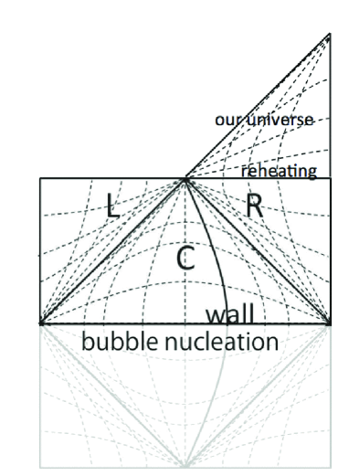
Figure 1: Penrose diagram of the universe after bubble nucleation. Bubble nucleates on the Cauchy surface shown as a horizontal line. Region below the surface classically does not exist. The R-region is the open FLRW universe which experiences slow-roll inflation and reheating to become our universe.

Figure 2: Contour plot of $V(\sigma,\phi)=V_{\mathrm{tun}}(\sigma)+V_{\mathrm{infl}}(\sigma,\phi)$ for the values of the parameters, $\alpha=0.1$, $\sigma_{0}=2m_{pl}$, $M_{V}=0.2m_{pl}$, $\beta=0.1$, $m_{\phi}=10^{-6}m_{pl}$, $\phi_{0}=15m_{pl}$. The contours are in Planck units. The false vacuum is located near $(\sigma_{0},\phi_{0})=(2m_{pl},15m_{pl})$, and the true vacuum is located at $(\sigma,\phi)=(0,0)$ which is not in the graph. The scalar fields tunnel from the false vacuum to the other side of the potential barrier. Then $\sigma$ undergoes rapid damped oscillations while $\phi$ slowly rolls down towards the true vacuum: See Sec. III.2 and III.3.

III Multi-field open inflation model

We now construct a concrete one-bubble multi-field open inflation model motivated by string landscape. In Sec. III.1, we propose a two-field system with a simple potential which satisfies requirements for a successful open inflation model. Then, in Sec. III.2, we explicitly obtain a multi-field instanton for the potential proposed in Sec. III.1. Finally, in Sec. III.3, using thus obtained instanton in Sec. III.2 as the initial condition, we solve the evolution of the universe inside the bubble until the end of slow-roll inflation. We find that the one-bubble open inflation scenario is indeed successfully realized in the system proposed in Sec. III.1.

III.1 Potential

Let us consider multi-field open inflation in a two-field system. Inspired by Linde:1995xm , we consider the case where one of the scalar fields $\sigma$ plays a major role in tunneling and and the other $\phi$ in slow-roll inflation inside the bubble. To realize such a situation, we split the potential $V(\sigma,\phi)$ to two parts as

$$V(\sigma,\phi) =V_{\mathrm{tun}}(\sigma)+V_{\mathrm{infl}}(\sigma,\phi)\,,$$ (15)

and assume that $V_{\mathrm{tun}}(\sigma)$ essentially determines the tunneling from the false vacuum, and that $V_{\mathrm{infl}}(\sigma,\phi)$ dominates the dynamics of slow-roll inflation after tunneling. To stabilize the false vacuum, $V_{\mathrm{infl}}(\sigma_{F},\phi)$ should give a large mass for $\phi$ around the false vacuum. On the other hand, after the tunneling, $\sigma$ should reach its true vacuum value $\sigma=\sigma_{T}$ sufficiently fast and $V_{\mathrm{infl}}(\sigma_{T},\phi)$ should give a potential for slow-roll inflation. We also assume that the number of $e$-folds of this slow-roll inflation is about $60$, as suggested by the string landscape argument Freivogel:2005vv . This constrains the initial value of $\phi$ after tunneling.

Now, we will construct a concrete form of the potential which satisfies the above requirements. With regard to $V_{\mathrm{tun}}(\sigma)$, we consider a simple quartic potential,

$$V_{\mathrm{tun}}(\sigma) =\alpha\sigma^{2}\left\{\left(\sigma-\sigma_{0}\right)^{2}+M_{V}^{2}\right\},$$ (16)

where the parameters are $\alpha$, $\sigma_{0}$ and $M_{V}$. This potential is in the same form as the potential (1), but here we consider the range of the parameters in the context of the string landscape. The parameter $\alpha$ is a quartic self-coupling constant which we assume $\alpha=O(1)$. In the string landscape, the characteristic energy scale is expected to be the Planck scale. Hence we assume $\sigma_{0}$ and $M_{V}$ are $O(m_{pl})$. In order to realize two minima in the potential $V_{\mathrm{tun}}(\sigma)$, we require the condition, $M_{V}\lesssim\sigma_{0}$.

It is known that a CDL instanton for $V_{\mathrm{tun}}(\sigma)$ does not always exist even when there is a false vacuum. Roughly speaking the existence of a CDL instanton depends on whether the absolute value of the second derivative of the potential $|V_{\mathrm{tun},\sigma\sigma}(\sigma)|$ is larger than the squared Hubble parameter at the top of the barrier $H^{2}(\sigma)=V_{\mathrm{tun}}(\sigma)/(3m_{pl}^{2})$, or more precisely, $|V_{\mathrm{tun},\sigma\sigma}(\sigma)|>4H^{2}(\sigma)$ at $\sigma=\sigma_{top}$ Jensen:1983ac ; Linde:1995xm . This condition can be understood by recalling that the wall thickness of an instanton is $\Delta r\sim|V_{\mathrm{tun},\sigma\sigma}(\sigma_{top})|^{-1/2}$ while the size of the Euclidean 4-sphere is $r\sim\pi/H(\sigma_{top})$. In order for an instanton to be fitted in the Euclidean sphere, we need $\Delta r<r$, which is the condition for the existence of a CDL instanton. When this condition is violated, instead of a CDL instanton we obtain HM instanton, which is a trivial classical path staying on the top of the potential barrier Hawking:1981fz . Since it is not easy to realize open inflation successfully when the system has only a HM instanton, as mentioned in Sec. I, we concentrate on the case where a CDL instanton exists in what follows. Although in a multi-field system the condition for the existence of a CDL instanton may be modified from the single-field case, here we impose $\sigma_{0}\lesssim 3m_{pl}$ from the condition of the existence of a single CDL instanton,

$$\left|V_{\mathrm{tun},\sigma\sigma}(\sigma_{top})\right|>4H^{2}(\sigma_{top})\,.$$ (17)

We will come back to this issue later in Sec. IV.

Let us consider the part of the potential that is supposed to govern the slow-roll inflation, $V_{\mathrm{infl}}(\sigma,\phi)$. We again restrict it to be at most quartic. With this requirement, we set

$$V_{\mathrm{infl}}(\sigma,\phi) =\frac{1}{2}m_{\phi}^{2}\phi^{2}+\frac{\beta}{2}\sigma^{2}\left(\phi-\phi_{0}\right)^{2},$$ (18)

where the parameters are $\beta$, $m_{\phi}$ and $\phi_{0}$. We assume $\beta=O(1)$.

For the potential given by the sum of Eqs. (16) and (18), let us compute the positions of the true vacuum and the false vacuum. It is easy to see that the true vacuum is at $(\sigma_{T},\phi_{T})=(0,0)$ where $V(\sigma_{T},\phi_{T})=0$. On the other hand, since there is a coupling between $\sigma$ and $\phi$, the exact position of the false vacuum is not so easy to obtain analytically. Here we assume $M_{V}^{2}\ll\sigma_{0}^{2}$ and $m_{\phi}^{2}\ll\beta\sigma_{0}^{2}$. Then one can employ a perturbative expansion, and at leading order the false vacuum is found to be at $(\sigma_{F},\phi_{F})\sim\left(\sigma_{0},\phi_{0}\right)$ with the vacuum energy given by $V(\sigma_{F},\phi_{F})\sim\alpha\sigma_{0}^{2}M_{V}^{2}+m_{\phi}^{2}\phi_{0}^{2}/2$ (see Appendix A for details). For simplicity, we restrict ourselves to this case in the following.

In order not to produce too much curvature perturbations from the slow-roll inflation, the inflaton mass, $m_{\phi}$, should be less than about $10^{-6}m_{pl}$ Komatsu:2010fb . For the number of $e$-folds of about $60$, the initial value of $\phi$ should then be about $15m_{pl}$. Thus we take $\phi_{0}\sim 15m_{pl}$ anticipating that the inflaton field does not move much during the tunneling. This is justified by the calculation in Sec. III.2. The actual number of $e$-folds is also explicitly calculated in Sec. III.3.

As mentioned in the beginning of this section, we also require that the mass square of the inflaton at false vacuum is larger than the Hubble square at the false vacuum, $V_{\phi\phi}(\sigma_{F},\phi_{F})\gg V(\sigma_{F},\phi_{F})/(3m_{pl}^{2})$, to ensure the picture of the false vacuum decay. If the mass is smaller than the Hubble parameter at the false vacuum, the quantum fluctuations dominate the motion of the scalar fields and the picture of the quantum tunneling from a false vacuum ceases to be valid. An investigation of this case may be of interest but beyond the scope of the present paper. This condition implies $\alpha M_{V}^{2}/m_{pl}^{2}<\beta$ under the assumptions discussed above that $m_{\phi}<10^{-6}m_{pl}$, $\alpha=O(1)$, $\beta=O(1)$, $\phi_{0}=O(m_{pl})$ and $\sigma_{0}=O(m_{pl})$.

In the construction of a potential for one-bubble open inflation, two conditions are to be satisfied at the same time. One is the condition for the tunneling through a CDL instanton, and the other is the condition for slow-roll inflation after tunneling. For a single-field system, a very artificial potential is necessary to fulfill both conditions at the same time Linde:1998iw . However, as discussed above and will be shown below, both conditions can be relatively easily satisfied with a simple quartic potential in a two-field model, by assigning the roles of tunneling and slow-rolling to two different fields. A contour plot of the potential $V(\sigma,\phi)=V_{\mathrm{tun}}(\sigma)+V_{\mathrm{infl}}(\sigma,\phi)$ for a set of the parameters that lead to a successful model of open inflation constructed in the following subsections is depicted in Fig. 2.

III.2 Calculation of an instanton

We apply the extended CDL method formulated in Sec. II to our model proposed in Sec. III.1. It should be noted that since the boundary conditions (9) are given at two different values of $t$, the existence of a non-trivial solution that satisfies the boundary conditions is confirmed only after one succeeds in explicitly constructing such a solution. We have searched for an instanton numerically with a shooting method for the parameters $\alpha=0.1$, $\sigma_{0}=2m_{pl}$, $M_{V}=0.2m_{pl}$, $\beta=0.1$, $m_{\phi}=10^{-6}m_{pl}$, $\phi_{0}=15m_{pl}$ and found an instanton. The above parameter set satisfies the conditions discussed in Sec. III.1. The behavior of $\sigma$, $\phi$ and $a$ of thus obtained instanton is shown in Fig. 3.

From Fig. 3, one sees that the scalar fields tunnel to the state $(\bar{\sigma}(0),\bar{\phi}(0))\sim(0,\phi_{0})$, and the inflaton does not move significantly during tunneling as expected in Sec. III.1. Thus the inflaton starts rolling down from about $\phi_{0}=15m_{pl}$ inside the nucleated bubble. The evolution of the universe after tunneling is explicitly calculated in Sec. III.3.

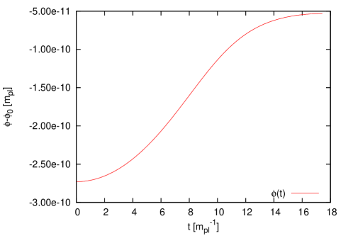
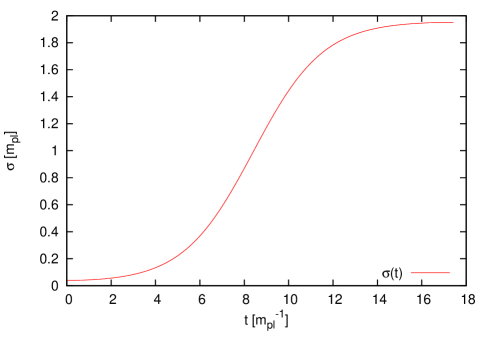
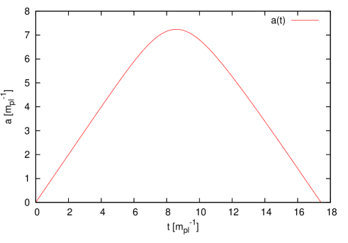
Figure 3: Multi-field instanton with gravity. The upper panel shows $\bar{\phi}(t)$. The lower-left and lower-right panels show $\bar{\sigma}(t)$ and $\bar{a}(t)$, respectively. The potential is given by Eq. (15), (16), and (18), with the parameters $\alpha=0.1$, $\sigma_{0}=2m_{pl}$, $M_{V}=0.2m_{pl}$, $\beta=0.1$, $m_{\phi}=10^{-6}m_{pl}$, and $\phi_{0}=15m_{pl}$.

III.3 Evolution after the tunneling

As discussed in Sec. II, the universe inside the bubble is an open FLRW universe, corresponding to the R-region in Fig. 2, with the metric given by the second line of Eq. (11). We have numerically calculated the evolution inside the bubble by solving the field equations (13) with the initial conditions $a_{R}(0)=0$ and $(\sigma_{R}(0),\phi_{R}(0))=(\bar{\sigma}(0),\bar{\phi}(0))$ at $t_{R}=0$.

The result is plotted in Fig. 4. In order to understand the evolution of the open universe, we decompose the Hubble square $H^{2}\equiv(\dot{a}_{R}/a_{R})^{2}$ into three contributions from $\phi$, $\sigma$ and the spatial curvature. We denote these contributions by $H_{\phi}^{2}$, $H_{\sigma}^{2}$ and $H_{k}^{2}$, respectively. Their explicit definitions are

$$H_{\phi}^{2} =\frac{1}{3m_{pl}^{2}}\left(\frac{1}{2}{\dot{\phi}_{R}}^{2}+V\left(\sigma_{T},\phi_{R}\right)\right)\,,$$

$$H_{\sigma}^{2} =\frac{1}{3m_{pl}^{2}}\left(\frac{1}{2}{\dot{\sigma}_{R}}^{2}+V\left(\sigma_{R},\phi_{R}\right)-V\left(\sigma_{T},\phi_{R}\right)\right)\,,$$

$$H_{k}^{2} =\frac{1}{a_{R}^{2}}\,.$$ (19)

Although the universe is curvature dominated right after tunneling, the contribution from the spatial curvature, $H_{k}^{2}$, eventually decays as $a_{R}^{-2}$, and the contribution from the inflaton field, $H_{\phi}^{2}$, starts to dominate, since $H_{\phi}^{2}$ can be well approximated as a constant. This happens at $a=a_{R0}$, where $a_{R0}\approx 1/H_{\phi}(0)$. We define the number of $e$-folds as $N=\ln(a_{R}(t_{R})/a_{R0})$. With this choice of $a_{R0}$, the inflation starts at $N=0$.

One can see that the contribution from the tunneling field, $H_{\sigma}^{2}$, is larger than that from the inflaton field, $H_{\phi}^{2}$, and smaller than that from the spatial curvature, $H_{k}^{2}$, right after tunneling. In the beginning $H^{2}$ decays as $1/a_{R}^{2}$, and the mass of the tunneling field becomes larger than the Hubble parameter at $a_{R}\approx V_{{\rm tun},\sigma\sigma}^{-1/2}$. After this epoch, $\sigma$ behaves as a non-relativistic matter and $H_{\sigma}^{2}$ decays rapidly as $a_{R}^{-3}$. Thus, $H_{\sigma}^{2}$ becomes much smaller than $H_{\phi}^{2}$ before the curvature dominated era ends at $N=0$. Thus $\sigma$ does not give any significant effect on the evolution of the universe.

Once $H_{\phi}^{2}$ becomes dominant, slow-roll inflation begins and lasts for about 60 $e$-folds. We suppose that the standard reheating process occurs when inflation ends. Note that since the contribution of $\sigma$ to the dynamics is small anyway, the evolution inside the bubble is similar even if we choose the parameter set that gives $H_{\sigma}^{2}<H_{\phi}^{2}$ right after tunneling.

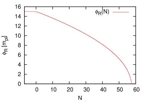
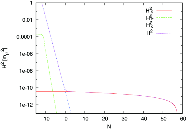
Figure 4: Upper panels: The time evolution of the inflaton field $\phi$ (upper-left) and the tunneling field $\sigma$ (upper-right) after tunneling as functions of $N\equiv\ln(a_{R}(t_{R})/a_{R0})$ with $a_{R0}$ being the value of the scale factor at the beginning of inflation.
Bottom panel: The contribution of the tunneling field $\sigma$, the inflaton field $\phi$, and the spatial curvature to the Hubble parameter as functions of $N$. $H_{\phi}$ , $H_{\sigma}$ and $H_{k}$ are defined in Eq. (19).

Before concluding this section, we emphasize that the solution given in Sec. III.2 is the first explicitly obtained multi-field instanton with gravity for a simple potential, and the evolution solved in Sec. III.3 gives a successful model of open inflation where the multi-field dynamics is fully taken into account. This two-field model solves the problem in single-field models in which one had to assume quite an artificial potential Linde:1998iw .

In the past, two-field open-inflation models were studied by several authors (see e.g. Linde:1995xm ; GarciaBellido:1997te ; Yamamoto:1996qq ; Sasaki:1996qn ). In particular, the quantum fluctuations of the scalar fields and gravitational waves were discussed rather extensively. However, the multi-field dynamics was not properly taken into account in these previous studies. Although they may perhaps be justified if regarded as results at leading order approximations, because the roles of $\sigma$ and $\phi$ are fairly clearly separated, quantitative verifications are left for future study.

IV Effect of Multi-field Dynamics on Tunneling Rate

As one of the important effects of multi-field dynamics on the tunneling, we consider its effect on the tunneling rate $\Gamma\propto e^{-B}$. Related to this issue, we mention recent interesting papers on the tunneling rate in the context of the cosmic string landscape. Aguirre, Johnson and Larfors studied the effect of dilatonic coupling in multi-field systems Johnson:2008vn ; Aguirre:2009tp , and concluded that it may completely prohibit tunneling in a substantial part of the landscape. Tye and Wohns studied the effect of resonant tunneling Tye:2009rb , and argued that it may drastically enhance the tunneling rate and change the landscape. These effects surely deserve further study, but here we focus on the system whose potential form is defined in Sec. III.1, in which neither of the above effects is present.

To compare the tunneling rate in a single-field model with a multi-field model is rather non-trivial, simply because there is no unique one-to-one correspondence between a single-field model and a multi-field model. Here for a given two-field model, we compare it with a single-field model obtained by fixing the inflaton at the false vacuum $\phi=\phi_{F}$,

$$V^{(0)}(\sigma)\equiv V(\sigma,\phi_{F})\,,$$ (20)

where $V(\sigma,\phi)$ is given by Eq. (15), that is, the sum of $V_{\mathrm{tun}}(\sigma)$ and $V_{\mathrm{infl}}(\sigma,\phi)$ in Eqs. (16) and (18), respectively. We denote the instanton solution for this potential by $\{\bar{\sigma}_{0}(t),\bar{\phi}_{0},\bar{a}_{0}(t)\}$, where $\bar{\phi}_{0}=\phi_{F}$ and $\{\bar{\sigma}_{0}(t),\bar{a}_{0}(t)\}$. Then we consider the difference of the exponent of the tunneling rate per unit volume per unit time between the two-field case and the single-field case,

$$\Delta B=B-B_{0}\,,$$ (21)

where $B=B[\bar{\sigma},\bar{\phi},\bar{a}]$ as defined in Eq. (3) and $B_{0}\equiv B[\bar{\sigma}_{0},\bar{\phi}_{0},\bar{a}_{0}]$.

To gain insight into the multi-field effect, we then vary the inflaton mass $m_{\phi}$ in Eq. (18). This is because the inflaton would stay at the false vacuum in the limit $m_{\phi}\to 0$, while the inflaton dynamics during tunneling is non-negligible, if not substantial, for $m_{\phi}\neq 0$. As mentioned in Sec. III.1, for an one-bubble open inflation model to be viable, it should not produce too large quantum fluctuations, which implies the condition $m_{\phi}\lesssim 10^{-6}m_{pl}$. However, here we tentatively ignore this constraint and consider the case $m_{\phi}\gg 10^{-6}m_{pl}$ as well, in order to see the effect of the multi-field dynamics more clearly.

In Tables 1 and 2, we list $\Delta\sigma=\bar{\sigma}(t_{\mathrm{end}})-\bar{\sigma}(0)$, $\Delta\phi=\bar{\phi}(t_{\mathrm{end}})-\bar{\phi}(0)$, $B$, $B_{0}$, $B_{HM}$ and $\Delta B$, for the parameters $\alpha=0.1$, $\sigma_{0}=2m_{pl}$, $M_{V}=0.2m_{pl}$ and $\phi_{0}=15m_{pl}$ with two different values of $\beta$; $\beta=0.1$ and $0.01$. Here, $B_{HM}$ denotes the value of $B$ obtained for a HM instanton as a reference, where the action is evaluated at the saddle point between the false and true vacua, $(\sigma_{top},\phi_{top})$, where $V_{\sigma}(\sigma_{top},\phi_{top})=V_{\phi}(\sigma_{top},\phi_{top})=0$. It is listed there because as $m_{\phi}$ increases the CDL instanton approaches the HM instanton, and the CDL instanton ceases to exist for sufficiently large $m_{\phi}$, as discussed below.

From Tables 1 and 2, we see that $\Delta B$ is either negative or too small to evaluate within the accuracy of our computation. This implies that the tunneling rate always increases when the effect of the multi-field dynamics is taken into account, though the increase may be negligibly small in some cases. The smallness of $|\Delta B|$ when $m_{\phi}\lesssim 10^{-2}m_{pl}$ is due to the smallness in the variation of $\bar{\phi}(t)$, or $\Delta\phi$, during the tunneling process, as seen in the tables.

It should be noted that not only $\Delta B$ but also $B_{0}$ depends on $m_{\phi}$ as well as on $\beta$, since the single-field case is given by the potential (20) which depends both on $m_{\phi}$ and $\beta$. As mentioned in the beginning of this section, this may be regarded as a consequence of the non-uniqueness of a single-field model for a given multi-field model. This fact makes it difficult to make a quantitative statement about the effect of multi-field dynamics. Nevertheless, the fact that the multi-field dynamics makes the tunneling rate larger is not affected. Furthermore, if we fix the single-field case to be the limit $m_{\phi}\to 0$, which may be well approximated by the case of $m_{\phi}=10^{-6}m_{pl}$, and compare it with cases of larger $m_{\phi}$, we see that the decrease in $B$ is roughly inversely proportional to $\Delta\phi$ when its effect is appreciable.

We also see from Tables 1 and 2 that the CDL instanton approaches its corresponding HM instanton as $m_{\phi}$ increases. This is because $V(\sigma_{top},\phi_{top})$ increases as $m_{\phi}$ increases, while the second derivative of $V(\sigma_{top},\phi_{top})$ along the tunneling path does not change much. We know that the criterion for the existence of a CDL instanton in the single-field case is given by Eq. (17). A straightforward extension of this criterion to the multi-field case is

$$|V^{\prime\prime}|>4H^{2}\,,$$ (22)

where $V^{\prime\prime}$ is the second derivative along the steepest descent path at the saddle point, or the negative eigenvalue of the mass matrix,

$$V^{\prime\prime}=\frac{V_{\sigma\sigma}+V_{\phi\phi}-\sqrt{(V_{\sigma\sigma}-V_{\phi\phi})^{2}+4V_{\sigma\phi}^{2}}}{2}\,,$$ (23)

at the point $(\sigma_{top},\phi_{top})$, and

$$H^{2}=\frac{V(\sigma_{top},\phi_{top})}{3m^{2}_{pl}}\,.$$ (24)

The criterion (22) is found to be violated at $m_{\phi}>4.12\times 10^{-2}m_{pl}$ ($m_{\phi}>4.03\times 10^{-2}m_{pl}$) for $\beta=0.1$ ($\beta=0.01$). In fact, we see that an instanton for $m_{\phi}=4\times 10^{-2}m_{pl}$ is very close to a HM instanton both from the smallness of $\Delta\sigma$ and the closeness of the value of $B$ to $B_{HM}$. If we further increase $m_{\phi}$ beyond this critical value, the potential barrier between the false and true vacua disappears and the false vacuum ceases to exist. The disappearance of the false vacuum is found to occur at $m_{\phi}=13.4\times 10^{-2}m_{pl}$ ($m_{\phi}=8.1\times 10^{-2}m_{pl}$) for $\beta=0.1$ ($\beta=0.01$).

Qualitatively the fact that the multi-field dynamics increases the tunneling rate may be understood as follows. As the variation of $\phi$ is small compared to that of $\sigma$ in our model, the single-field approximation is valid at leading order. Now for a given single-field path $\{\sigma,a\}=\{\bar{\sigma}_{0}(t),\bar{a}_{0}(t)\}$, the dynamics of $\phi$ is determined by minimizing the action $S_{E}[\bar{\sigma}_{0}(t),\bar{a}_{0}(t),\phi]$. Then the action for a fixed value of $\phi$ would naturally be larger than that minimizes the action $S_{E}[\bar{\sigma}_{0}(t),\bar{a}_{0}(t),\phi]$. In the limit when the backreaction of the dynamics of $\phi$ on that of $\sigma$ and $a$ is small, the resulting value of the action will be equal to the action of the actual CDL instanton. Hence the effect of the multi-field dynamics is to decrease the value of the action, and hence increase the tunneling rate.

Physically, by taking into account the dynamics of $\phi$, the multi-field tunneling proceeds along the path where potential barrier is lower than the path along $\phi=\phi_{F}$. Thus the tunneling occurs more easily when the multi-field dynamics is taken into account. If we take the difference between the potential (18) and that at $\phi=\phi_{F}$, $\Delta V=V_{\mathrm{infl}}(\sigma,\phi)-V_{\mathrm{infl}}(\sigma,\phi_{F})$, we find that the potential energy along a multi-field tunneling path, which is away from $\phi_{F}$, decreases as $m_{\phi}$ increases or $\beta$ decreases. This explains the dependence of $\Delta B$ on $m_{\phi}$ and $\beta$ in Tables 1 and 2.

$m_{\phi}[m_{pl}]$	$\Delta\sigma[m_{pl}]$	$\Delta\phi[m_{pl}]$	$B$	$B_{0}$	$B_{HM}$	$\Delta B$
$10^{-6}$	$1.91$	$2.20\times 10^{-10}$	12109.11	12109.11	12679.69	$|\Delta B|<0.01$
$10^{-4}$	$1.91$	$2.20\times 10^{-6}$	12108.10	12108.10	12678.65	$|\Delta B|<0.01$
$10^{-3}$	$1.91$	$2.19\times 10^{-4}$	12008.71	12008.71	12576.67	$|\Delta B|<0.01$
$5\times 10^{-3}$	$1.90$	$5.34\times 10^{-3}$	9975.05	9975.07	10484.43	-0.02
$10^{-2}$	$1.87$	$1.97\times 10^{-2}$	6322.66	6322.85	6691.28	-0.19
$2\times 10^{-2}$	$1.73$	$6.00\times 10^{-2}$	2188.07	2189.41	2305.67	-1.35
$3\times 10^{-2}$	$1.38$	$8.73\times 10^{-2}$	849.20	852.07	868.55	-2.87
$4\times 10^{-2}$	$0.49$	$4.58\times 10^{-2}$	372.15	376.39	372.28	-4.25

Table 1: The values of several quantities of interest for different values of $m_{\phi}$. $\Delta\sigma=\bar{\sigma}(t_{\mathrm{end}})-\bar{\sigma}(0)$ is the total variation of $\sigma$ during the tunneling, and $\Delta\phi=\bar{\phi}(t_{\mathrm{end}})-\bar{\phi}(0)$ is that of $\phi$. $B$, $B_{0}$ and $B_{HM}$ are the values of the bounce action for the full multi-field instanton, for the corresponding single-field instanton, and for the corresponding HM instanton, respectively, and $\Delta B=B-B_{0}$. The model parameters are $\alpha=0.1$, $\sigma_{0}=2m_{pl}$, $M_{V}=0.2m_{pl}$, $\phi_{0}=15m_{pl}$ and $\beta=0.1$.

$m_{\phi}[m_{pl}]$	$\Delta\sigma[m_{pl}]$	$\Delta\phi[m_{pl}]$	$B$	$B_{0}$	$B_{HM}$	$\Delta B$
$10^{-6}$	1.91	$3.20\times 10^{-10}$	12109.11	12109.11	12679.69	$|\Delta B|<0.01$
$10^{-4}$	1.91	$3.20\times 10^{-6}$	12108.10	12108.10	12678.65	$|\Delta B|<0.01$
$10^{-3}$	1.91	$3.20\times 10^{-4}$	12008.71	12008.71	12576.67	$|\Delta B|<0.01$
$5\times 10^{-3}$	1.90	$7.72\times 10^{-3}$	9975.96	9976.06	10485.40	-0.10
$10^{-2}$	1.87	$2.79\times 10^{-2}$	6328.61	6329.83	6697.90	-1.23
$2\times 10^{-2}$	1.73	$7.86\times 10^{-2}$	2196.44	2205.89	2316.09	-9.44
$3\times 10^{-2}$	1.37	$1.04\times 10^{-1}$	844.13	865.98	863.91	-21.84
$4\times 10^{-2}$	0.24	$2.53\times 10^{-2}$	350.32	383.60	350.33	-33.28

Table 2: Same as Table 1, but for $\beta=0.01$.

It is then natural to conjecture that the multi-field dynamics tends to increase the tunneling rate in general. The reason is that although the action for a multi-field instanton is not a minimum but a saddle point of the Euclidean action, there is only a single negative direction that decreases the action. In other words, if we can effectively separate out the dynamical degrees of freedom orthogonal to the tunneling path, the activation of any of these degrees of freedom would increase the value of the action. Hence freezing out these degrees of freedom by hand would result in the increase of the action. Conversely the inclusion of the dynamics of these degrees of freedom would decrease the value of the action.

V Conclusion and Discussion

In this paper, motivated by string landscape we have studied the dynamics of multi-field open inflation. We have considered a system of two scalar fields, in which one of the fields is to play a major role in quantum tunneling from a false vacuum, and is called the tunneling field, and the other to play a major role in the subsequent slow-roll inflation inside the bubble, and hence called the inflaton field. For definiteness, we have considered the case when the slow-roll inflation is of chaotic type, that is, a large-field model of inflation. The introduction of two fields solves the difficulty in a single-field open inflation model in which quite an artificial potential was necessary to realize both tunneling and the subsequent slow-roll inflation Linde:1998iw . In our model the potential is a simple polynomial of quartic order in the scalar fields. No fine-tuning of the parameters has been necessary, although a certain degree of tuning has been needed to satisfy the constraint that the number of $e$-folds of inflation should be about 60, as well as the standard requirement that the amplitude of scalar perturbations should not exceed $10^{-5}$.

We have solved the Euclidean equations of motion numerically to obtain the multi-field instanton explicitly. Then by analytically continuing the instanton solution, we have solved the evolution inside the bubble. We have confirmed that our model is a viable open inflation model which can give the present curvature parameter $\Omega_{K,0}\sim 10^{-2}-10^{-3}$. Thus our model is the first concrete, viable model of open inflation with a simple potential, if not realistic.

Then in order to understand the effect of the multi-field dynamics on quantum tunneling, we have considered the tunneling rate. For a given two-field model, we have considered a corresponding single-field model by fixing the value of the inflaton at the false vacuum value, and compared the tunneling rates of the two models. We have found that the multi-field dynamics always increases the tunneling rate provided that the multi-field effect is perturbative. This may be understood physically as a result of the fact that the multi-field tunneling occurs along a classical path where the potential barrier is lower than the corresponding single-field case in which the value of one of the fields is fixed by hand.

It should be noted that in Johnson:2008vn ; Aguirre:2009tp it was concluded that multi-field tunneling between two vacua by an O(4)-symmetric instanton can be totally prohibited. However, as mentioned in Sec. I, this apparently opposite result can be understood by noting the difference in the model considered there from ours. This can be regarded as an example of highly non-trivial aspects of the multi-field tunneling. In order to understand the string landscape we definitely need further studies of multi-field tunneling.

In this paper, we have straightforwardly extended the CDL instanton method for the single-field tunneling with gravity to the multi-field case. However, the CDL instanton method itself has some subtle points as mentioned in Sec. II. One of the most important issues is the physical interpretation of a CDL instanton. Since the topology of a CDL instanton is $S^{4}$ the boundary conditions are determined by the regularity of the solution. Hence there is no region in the solution where the false vacuum is attained. This is in marked contrast with the flat space case in which the topology is $E^{4}$ and the instanton approaches the false vacuum asymptotically at infinity. This raises a question about the physical interpretation of an CDL instanton that if it really describes the false vacuum decay. In particular, in the limiting case a CDL instanton ceases to exist and there is only a HM instanton which sits at the top of the barrier. In this case, the analytic continuation of the solution does not give the classical evolution after tunneling unless quantum fluctuations are taken into account.

It is important to discuss the observational implications of multi-field open inflation models. As far as the model we have constructed is concerned, the dynamics of the tunneling field turns out to be unimportant inside the bubble. That is, the dynamics inside the bubble is essentially that of single-field chaotic inflation. Then we can calculate the power spectrum of the quantum fluctuations by using the known formulation in the literature Garriga:1997wz without any modification. The expected result is that there is a slight suppression of the curvature perturbation on scales comparable to the curvature scale. However, since $\Omega_{K,0}\lesssim 10^{-2}$, this effect on CMB, say, is probably buried under the cosmic variance.

For models in which the energy scale of the false vacuum is much higher, closer to the Planck scale, it was discussed that the trace of the false vacuum could be observationally detected Yamauchi:2011qq . It remains to be seen if such a model can be constructed in the multi-field context with relatively a simple potential.

Another interesting possibility is a model in which the tunneling field would remain non-trivial inside the bubble to produce isocurvature perturbations or in which damped oscillations of the tunneling field is delayed to induce interesting features in the power spectrum.

Furthermore, since the quantum state inside the bubble is known to be modified from the Bunch-Davis vacuum in general Yamamoto:1996qq ; Garriga:1997wz , it is interesting to see if there is any multi-field model in which this modification can be observable, say, in the CMB bispectrum Meerburg:2009ys .

If any of these possible models can be constructed in the context of string landscape, it will provide a good observational test of the string landscape. We hope to come back to these issues in the near future.

Appendix A properties of the potential

In this Appendix, we briefly summarize the properties of the potential defined in Eqs. (15), (16), and (18). Let us recapitulate them,

$$V(\sigma,\phi) = V_{\mathrm{tun}}(\sigma)+V_{\mathrm{infl}}(\sigma,\phi)\,;$$ (28)

$$V_{\mathrm{tun}}(\sigma)=\alpha\sigma^{2}\left\{\left(\sigma-\sigma_{0}\right)^{2}+M_{V}^{2}\right\}\,,$$

$$V_{\mathrm{infl}}(\sigma,\phi)=\frac{1}{2}m_{\phi}^{2}\phi^{2}+\frac{\beta}{2}\sigma^{2}\left(\phi-\phi_{0}\right)^{2}\,.$$

Since the potential is quartic and non-negative, there is at least one minimum. To see the conditions for the existence of two minima, we calculate the first derivatives of the potential:

$$V_{\sigma}=2\sigma\biggl{[}\alpha\left\{2\left(\sigma-\sigma_{0}\right)^{2}+\sigma_{0}\left(\sigma-\sigma_{0}\right)+M_{V}^{2}\right\}+\frac{1}{2}\beta\left(\phi-\phi_{0}\right)^{2}\biggr{]}\,,$$ (29)

$$V_{\phi}=m_{\phi}^{2}\phi+\beta\sigma^{2}\left(\phi-\phi_{0}\right)\,,$$ (30)

and the second derivatives:

$$V_{\sigma\sigma}=12\alpha\biggl{[}\sigma\left(\sigma-\sigma_{0}\right)+\frac{1}{6}\left(\sigma_{0}^{2}+M_{V}^{2}\right)\biggr{]}+\beta\left(\phi-\phi_{0}\right)^{2}\,,$$ (31)

$$V_{\sigma\phi}=2\beta\sigma\left(\phi-\phi_{0}\right)\,,$$ (32)

$$V_{\phi\phi}=m_{\phi}^{2}+\beta\sigma^{2}\,.$$ (33)

It is easy to see that there is a minimum at $(\sigma,\phi)=(0,0)$. Since $V\geq 0$, it is the global minimum.

On the other hand, it is not easy to spell out the condition for the existence of a false vacuum analytically. In general we have to resort to a numerical method. Nevertheless, if the conditions $M_{V}^{2}\ll\sigma_{0}^{2}$ and $m_{\phi}^{2}\ll\beta\sigma_{0}^{2}$ are both satisfied, we find by an inspection of Eqs. (30), together with Eqs. (33), that there is a local minimum at

$$(\sigma,\phi)=\left(\sigma_{0}\left[1+O\left(\frac{M_{V}^{2}}{\sigma_{0}^{2}}\right)\right],\phi_{0}\left[1+O\left(\frac{m_{\phi}^{2}}{\beta\sigma_{0}^{2}}\right)\right]\right).$$ (34)

A more careful, perturbative analysis gives the position of the false vacuum and the vacuum energy as

$$\sigma_{F} =\sigma_{0}\left[1-\frac{M_{V}^{2}}{\sigma_{0}^{2}}-2\left(\frac{M_{V}^{2}}{\sigma_{0}^{2}}\right)^{2}-\frac{\beta\phi_{0}^{2}}{2\alpha\sigma_{0}^{2}}\left(\frac{m_{\phi}^{2}}{\beta\sigma_{0}^{2}}\right)^{2}+O(\epsilon^{3})\right]\,,$$

$$\phi_{F} =\phi_{0}\left[1-\frac{m_{\phi}^{2}}{\beta\sigma_{0}^{2}}+\left(\frac{m_{\phi}^{2}}{\beta\sigma_{0}^{2}}\right)^{2}-2\left(\frac{m_{\phi}^{2}}{\beta\sigma_{0}^{2}}\right)\left(\frac{M_{V}^{2}}{\sigma_{0}^{2}}\right)+O(\epsilon^{3})\right]\,,$$

$$V(\sigma_{F},\phi_{F}) =\alpha\sigma_{0}^{2}M_{V}^{2}\left[1-2\frac{M_{V}^{2}}{\sigma_{0}^{2}}+O(\epsilon^{2})\right]+\frac{1}{2}m_{\phi}^{2}\phi_{0}^{2}\left[1-2\frac{m_{\phi}^{2}}{\beta\sigma_{0}^{2}}+O(\epsilon^{2})\right]\,.\,$$ (35)

where we have assumed ${M_{V}^{2}}/{\sigma_{0}^{2}}=O(\epsilon)$ and ${m_{\phi}^{2}}/(\beta\sigma_{0}^{2})=O(\epsilon)$ with $\epsilon$ being a small parameter.

The false vacuum disappears when the equations $V_{\sigma}=V_{\phi}=0$ cease to have a real solution other than $\sigma=\phi=0$. Then from the first of Eqs. (30), one finds that, under the assumption $\epsilon\ll 1$, a sufficient condition for the existence of a false vacuum is

$$\left(\frac{\beta\phi_{0}^{2}}{\alpha\sigma_{0}^{2}}\right)\left(\frac{m_{\phi}^{2}}{\beta\sigma_{0}^{2}}\right)\lesssim 1\quad\leftrightarrow\quad m_{\phi}^{2}\phi_{0}^{2}\lesssim\alpha\sigma_{0}^{4}\,.$$ (36)

From the last expression of Eqs. (35), one sees that the contribution to the false vacuum energy from $V_{\mathrm{infl}}(\sigma,\phi)$ becomes comparable to that from $V_{\mathrm{tun}}(\sigma)$ when $\alpha\sigma_{0}^{2}M_{V}^{2}\sim m_{\phi}^{2}\phi_{0}^{2}$. However, in the case of a model we constructed in Sec. III, the parameters satisfy the inequality $\alpha\sigma_{0}^{2}M_{V}^{2}\gg m_{\phi}^{2}\phi_{0}^{2}$. Hence the inflaton potential $V_{\mathrm{infl}}$ plays only a minor role in the instanton solution, that is, in the quantum tunneling.

References

- (1) S. R. Coleman, Phys. Rev. D15, 2929-2936 (1977).
- (2) S. R. Coleman, F. De Luccia, Phys. Rev. D21, 3305 (1980).
- (3) S. Kachru, R. Kallosh, A. D. Linde, S. P. Trivedi, Phys. Rev. D68, 046005 (2003). [hep-th/0301240].
- (4) L. Susskind, In *Carr, Bernard (ed.): Universe or multiverse?* 247-266. [hep-th/0302219].
- (5) B. Freivogel, L. Susskind, Phys. Rev. D70, 126007 (2004). [hep-th/0408133].
- (6) B. Freivogel, M. Kleban, M. Rodriguez Martinez, L. Susskind, JHEP 0603, 039 (2006). [hep-th/0505232].
-
(7)
M. Bucher, A. S. Goldhaber and N. Turok,
Phys. Rev. D 52, 3314 (1995)
[arXiv:hep-ph/9411206].
M. Bucher and N. Turok, Phys. Rev. D 52, 5538 (1995) [arXiv:hep-ph/9503393]. - (8) M. Sasaki, T. Tanaka, K. Yamamoto, Phys. Rev. D51, 2979-2995 (1995). [gr-qc/9412025].
-
(9)
A. D. Linde,
Phys. Lett. B351, 99-104 (1995).
[hep-th/9503097].
A. D. Linde, A. Mezhlumian, Phys. Rev. D52, 6789-6804 (1995). [astro-ph/9506017]. -
(10)
K. Yamamoto, M. Sasaki, T. Tanaka,
Astrophys. J. 455, 412-418 (1995).
[astro-ph/9501109].
T. Tanaka, M. Sasaki, Prog. Theor. Phys. 97, 243-262 (1997). [astro-ph/9701053].
M. Sasaki, T. Tanaka and Y. Yakushige, Phys. Rev. D 56, 616 (1997) [arXiv:astro-ph/9702174].
T. Tanaka and M. Sasaki, Phys. Rev. D 59, 023506 (1999) [arXiv:gr-qc/9808018].
A. M. Green, A. R. Liddle, Phys. Rev. D55, 609-615 (1997). [astro-ph/9607166].
J. Garcia-Bellido, Phys. Rev. D56, 3225-3237 (1997). [astro-ph/9702211].
A. D. Linde, M. Sasaki and T. Tanaka, Phys. Rev. D 59, 123522 (1999) [arXiv:astro-ph/9901135]. - (11) K. Yamamoto, M. Sasaki, T. Tanaka, Phys. Rev. D54, 5031-5048 (1996). [astro-ph/9605103].
- (12) M. Sasaki, T. Tanaka, Phys. Rev. D54, 4705-4708 (1996). [astro-ph/9605104].
-
(13)
J. Garcia-Bellido, J. Garriga, X. Montes,
Phys. Rev. D57, 4669-4685 (1998).
[hep-ph/9711214].
J. Garriga, V. F. Mukhanov, Phys. Rev. D56, 2439-2441 (1997). [astro-ph/9702201].
J. Garcia-Bellido, J. Garriga, X. Montes, Phys. Rev. D60, 083501 (1999). [hep-ph/9812533]. - (14) D. Yamauchi, A. Linde, A. Naruko, M. Sasaki and T. Tanaka, Phys. Rev. D 84, 043513 (2011) [arXiv:1105.2674 [hep-th]].
- (15) A. D. Linde, Phys. Rev. D 59, 023503 (1999) [arXiv:hep-ph/9807493].
- (16) S. W. Hawking and I. G. Moss, Phys. Lett. B 110, 35 (1982).
- (17) L. G. Jensen and P. J. Steinhardt, Nucl. Phys. B 237, 176 (1984).
-
(18)
M. C. Johnson and M. Larfors,
Phys. Rev. D 78, 123513 (2008)
[arXiv:0809.2604 [hep-th]].
M. C. Johnson and M. Larfors, Phys. Rev. D 78, 083534 (2008) [arXiv:0805.3705 [hep-th]]. - (19) A. Aguirre, M. C. Johnson and M. Larfors, Phys. Rev. D 81, 043527 (2010) [arXiv:0911.4342 [hep-th]].
- (20) S. R. Coleman, V. Glaser and A. Martin, Commun. Math. Phys. 58, 211 (1978).
- (21) R. Bousso and A. Chamblin, Phys. Rev. D 59, 084004 (1999) [arXiv:gr-qc/9803047].
- (22) V. A. Rubakov and S. M. Sibiryakov, Theor. Math. Phys. 120, 1194 (1999) [Teor. Mat. Fiz. 120, 451 (1999)] [arXiv:gr-qc/9905093].
- (23) U. Gen and M. Sasaki, Phys. Rev. D 61, 103508 (2000) [arXiv:gr-qc/9912096].
- (24) E. Komatsu et al. [WMAP Collaboration], Astrophys. J. Suppl. 192, 18 (2011) [arXiv:1001.4538 [astro-ph.CO]].
-
(25)
S. -H. H. Tye, D. Wohns,
[arXiv:0910.1088 [hep-th]].
S. -H. H. Tye, D. Wohns, [arXiv:1106.3075 [cond-mat.other]]. -
(26)
J. Garriga, X. Montes, M. Sasaki and T. Tanaka,
Nucl. Phys. B 513, 343 (1998)
[arXiv:astro-ph/9706229].
J. Garriga, X. Montes, M. Sasaki and T. Tanaka, Nucl. Phys. B 551, 317 (1999) [arXiv:astro-ph/9811257]. - (27) P. D. Meerburg, J. P. van der Schaar and P. S. Corasaniti, JCAP 0905, 018 (2009) [arXiv:0901.4044 [hep-th]].