‘Similar’ coordinate systems and the Roche geometry. Application

Abstract

A new equivalence relation, named relation of ’similarity’ is defined and applied in the restricted three-body problem. Using this relation, a new class of trajectories (named ’similar’ trajectories) are obtained; they have the theoretical role to give us new details in the restricted three-body problem. The ‘similar’ coordinate systems allow us in addition to obtain a unitary and an elegant demonstration of some analytical relations in the Roche geometry. As an example, some analytical relations published in Astrophysical Journal by Seidov in 2004 are demonstrated.

1 Introduction

In the frame of the restricted three-body problem, the Roche geometry is a fundamental notion, and it is much studied, using for this aim different coordinate systems.

The usual way of treating the problem of motion of test particle and the Roche geometry in the gravitational field of a binary system consists in introducing a coordinate system (xyz), rotating jointly with the components. The x-axis passes through the centers of both components, and the y-axis is situated in the orbital plane; but there are more possibilities to locate the origin of the coordinate system. For example the origin can be located in the mass center of the binary system (Moulton, 1923), or in the center of the more massive star (Kopal, 1978, 1989; Roy, 1988; Szebehely, 1967). But there are some papers (Huang, 1967; Kruszewski, 1963), where the location of the origin of the coordinate system is not precisely indicated. For example Huang (1967) wrote: ”Thus, if we denote $1-\mu$ as the mass of one component, $\mu$ will be the mass of the other. Let us further choose a rotating (x,y,z) system such that the origin is at the center of the $1-\mu$ component, the x-axis points always towards the $\mu$ component, and the $xy$ plane coincides with the orbital plane.”

This way to locate the origin of the coordinate system is not an ambiguous one, but it offers the opportunity of the question: What happens with the equations of motion of the test particle and with the geometry of the equipotential curves, in the restricted three-body problem, if the origin of the coordinate system is taken in the center of the less massive star.

The aim of this paper is to answer the question above, by introducing a new notion: the ’similar’ coordinate systems.

In order to do so, a binary relation is created, which is denoted by the author as relation of ’similarity’. Then, using this relation, the ’similar’ coordinate systems, and the necessary ’similar’ parameters and physical quantities are defined, obtaining ’similar’ equations of motion, and ’similar’ equipotential curves.

The conclusion of this study is that the use of ’similar’ coordinate systems in the restricted three-body problem allows us to complete the traditional study of the Roche geometry with some new features.

2 Relation of ’similarity’

In this article we shall write ’similar’ (not similar), because we intend to use this word as the name of a new mathematical relation, and not as an adjective.

Definition: Two or more mathematical objects are in the ’similarity’ relation in connection with a given definition ($\mathcal{D}$), if the objects are completely characterized by $\mathcal{D}$.

For example:

1. in algebra: The numbers $x_{1}=1$ and $x_{2}=-3$ are ‘similar’ in connection with the definition: x is the solution of equation: $x^{2}+2x-3=0$, $x\in\mathbb{Z}$.

2. in geometry: If we consider the definition: P is the point situated into a given plane ($\pi$), at the distance $r=1$ from the given point A, $A\in(\pi)$, then all the points of the circle having the center A and radius $r=1$ are ’similar’.

3. in astrophysics: In the frame of the circular restricted three-body problem we define a comoving coordinate system situated in the orbital plane, having the origin in the center of one component of the binary system and the abscissa’s axis pointing to the other component. Then the coordinate systems $xS_{1}y$ and $x^{\prime}S_{2}y^{\prime}$ are ‘similar’ (see Figure 1). (In many books or articles of astronomy, this is the coordinate system’s definition used to study the restricted three-body problem (Huang, 1967), but usualy only $xS_{1}y$ coordinate system is considered. In 1963, Kruszewski wrote: ”The center of coordinates is placed at the center of the (arbitrarily chosen) primary component” (Kruszewski, 1963). This means that if the origin of the coordinate system is taken into the center of the secondary component, the results will be similar. In this article we try to find what this similarity implies.)

The study of the restricted three-body problem in ’similar’ coordinate systems follows the classical algorithm, but some typical peculiarities appear. So, the use of the ’similar’ coordinate systems impose the use of some physical and geometrical ’similar’ quantities:

- ’similar’ mass ratios $q$ and $q^{\prime}$

- ’similar’ distances $r_{1}$, $r_{2}$, $r_{1}^{\prime}$, and $r_{2}^{\prime}$

- ’similar’ initial velocities $v_{0x}$, $v_{0y}$, $v_{0x}^{\prime}$, and $v_{0y}^{\prime}$

- ’similar’ initial positions $x_{0}$, $y_{0}$, $x_{0}^{\prime}$, and $y_{0}^{\prime}$.

Of course, as in algebra the ’similar’ solutions of a polynomial equation are connected by the relations of Viète, the two ’similar’ coordinate systems are connected by the equations of coordinate transformations (see section 4).

It is easy to verify that the relation of ’similarity’ is reflexive, symmetric, and transitive. That means that the relation of ’similarity’ is an equivalence relation.

Remark:

1. The role of the definition into the establishment of a ’similarity’ is huge. So, if we consider the definition: x is the solution of equation: $x^{2}+2x-3=0$, $x\in\mathbb{N}$, the numbers $x_{1}=1$ and $x_{2}=-3$ are not ‘similar’.

2. The solutions of a problem (including the repeated ones) are in relation of ’similarity’, because these can be defined as satisfying the same problem.

3 ’Similar’ coordinate systems, ’similar’ parameters and physical quantities

In the frame of the circular, restricted three-body problem (Szebehely, 1967), we will consider $S_{1}$ and $S_{2}$ the components of a binary system, $m_{1}$ and $m_{2}$ their masses and $L_{i}$, $i=\overline{1,5}$ the Lagrangian points. Due to the normalization (see section 4), the distance between $S_{1}$ and $S_{2}$ is equal to 1. We will consider a rectangular coordinate system, so that one component of the binary star has coordinates (0,0,0), the other one has coordinates (1,0,0), and the angular Keplerian velocity $\vec{\omega}_{k}$ has components $(0,0,\omega_{k})$. We observe immediately that there are two coordinate systems: ($xS_{1}yz$) and ($x^{\prime}S_{2}y^{\prime}z^{\prime}$), which can be built. These are ‘similar’ coordinate systems (see Figure 1).

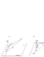
Figure 1: The ’similar’ coordinate systems with origin in $S_{1}$ and $S_{2}$ .

As it is well-known (Kopal, 1978) p.327-328, (Kopal, 1989) p.15-16 the mass ratio $q$ is the main parameter which describes the Roche geometry. If we denote $q$ = (mass which isn’t into the origin)/(mass which is into the origin), we have $q=\frac{m_{2}}{m_{1}}$ and $q^{\prime}=\frac{m_{1}}{m_{2}}$ which are ‘similar’ parameters. We denote $r_{1}$ = distance of the infinitesimal mass (Szebehely, 1967) to the origin of the coordinate system, and $r_{2}$ = distance of the infinitesimal mass to the star which is not into the origin. Therefore $r_{1}$ with $r_{1}^{\prime}$ and $r_{2}$ with $r_{2}^{\prime}$ are ‘similar’ distances (see Figure 1).

We have ”’similar’ velocities $v=\frac{dr_{1}}{dt}$ and $v^{\prime}=\frac{dr_{1}^{\prime}}{dt}$ and ’similar’ accelerations $a=\frac{d^{2}r_{1}}{dt^{2}}$ and $a^{\prime}=\frac{d^{2}r_{1}^{\prime}}{dt^{2}}$.

4 ’Similar’ equations of motion

The forces which act on infinitesimal mass $S_{3}$ are $\vec{F}_{grav1}$, $\vec{F}_{grav2}$, $\vec{F}_{centrif}$, and $\vec{F}_{Coriolis}$ (Szebehely, 1967) p.590). Their expressions in $(xS_{1}yz)$ and $(x^{\prime}S_{2}y^{\prime}z^{\prime})$ coordinate systems are:

$$\vec{F}_{grav1}=-\frac{Gm_{1}m_{3}x}{r_{1}^{3}}\;\vec{i}-\frac{Gm_{1}m_{3}y}{r_{1}^{3}}\;\vec{j}-\frac{Gm_{1}m_{3}z}{r_{1}^{3}}\;\vec{k}$$ (1)

$$\vec{F}_{grav2}=-\frac{Gm_{2}m_{3}[x-(R_{1}+R_{2})]}{r_{2}^{3}}\;\vec{i}-\frac{Gm_{2}m_{3}y}{r_{2}^{3}}\;\vec{j}-\frac{Gm_{2}m_{3}z}{r_{2}^{3}}\;\vec{k}$$ (2)

$$\vec{F}_{centrif}=m_{3}\,\omega_{k}^{2}\left[(x-R_{1})\vec{i}+y\vec{j}\right]$$ (3)

$$\vec{F}_{Coriolis}=2m_{3}\,\omega_{k}\left(\frac{dy}{dt}\vec{i}-\frac{dx}{dt}\vec{j}\right)$$ (4)

and respectively:

$$\vec{F^{\prime}}_{grav1}=-\frac{Gm_{2}m_{3}x^{\prime}}{r_{1}^{{}^{\prime}3}}\;\vec{i}-\frac{Gm_{2}m_{3}y^{\prime}}{r_{1}^{{}^{\prime}3}}\;\vec{j}-\frac{Gm_{2}m_{3}z^{\prime}}{r_{1}^{{}^{\prime}3}}\;\vec{k}$$ (5)

$$\vec{F^{\prime}}_{grav2}=-\frac{Gm_{1}m_{3}[x^{\prime}-(R_{1}+R_{2})]}{r_{2}^{{}^{\prime}3}}\;\vec{i}-\frac{Gm_{1}m_{3}y^{\prime}}{r_{2}^{{}^{\prime}3}}\;\vec{j}-\frac{Gm_{1}m_{3}z^{\prime}}{r_{2}^{{}^{\prime}3}}\;\vec{k}$$ (6)

$$\vec{F^{\prime}}_{centrif}=m_{3}\,\omega_{k}^{2}\left[(x^{\prime}-R_{2})\vec{i}+y^{\prime}\vec{j}\right]$$ (7)

$$\vec{F^{\prime}}_{Coriolis}=-2m_{3}\,\omega_{k}\left(\frac{dy^{\prime}}{dt}\vec{i}-\frac{dx^{\prime}}{dt}\vec{j}\right)$$ (8)

where $G$ is the gravitational constant.

$\vec{F}_{Coriolis}$ and $\vec{F^{\prime}}_{Coriolis}\,$ have opposite signs because of the orientation of vectors $\vec{\omega}_{k}\times\vec{v}$ and $\vec{\omega^{\prime}}_{k}\times\vec{v^{\prime}}$ (see Figure 2).

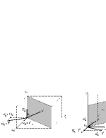
Figure 2: Explanation for the opposite signs of Coriolis force in the two ’similar’ coordinate systems .

By consequence in the $(xS_{1}yz)$ coordinate system the vectorial equation of motion is:

$$m_{3}\>\vec{a}=\vec{F}_{grav1}+\vec{F}_{grav2}+\vec{F}_{centrif}+\vec{F}_{Coriolis}$$ (9)

and in the $(x^{\prime}S_{2}y^{\prime}z^{\prime})$ coordinate system:

$$m_{3}\>\vec{a^{\prime}}=\vec{F^{\prime}}_{grav1}+\vec{F^{\prime}}_{grav2}+\vec{F^{\prime}}_{centrif}+\vec{F^{\prime}}_{Coriolis}$$ (10)

We shall use a special unit system (Kopal, 1978) p.318: we choose for the mass unit the sum of the masses of the components of the binary system, for the distance unit the distance between the centers of the components, and for the time unit the reciprocal of the angular Keplerian velocity. In that case, the orbital period will be $P=2\pi$, and $G=1$.

Then $m_{1}=\frac{1}{1+q}$, $m_{2}=\frac{q}{1+q}$, $R_{1}=\frac{q}{1+q}$, $R_{2}=\frac{1}{1+q}$.

Using the same unit system, the scalar equations of motion in the $(xS_{1}yz)$ coordinate system become:

$$\frac{d^{2}x}{dt^{2}}-2\frac{dy}{dt}=x-\frac{q}{1+q}-\frac{x}{(1+q)r_{1}^{3}}-\frac{q(x-1)}{(1+q)r_{2}^{3}}$$ (11)

$$\frac{d^{2}y}{dt^{2}}+2\frac{dx}{dt}=y-\frac{y}{(1+q)r_{1}^{3}}-\frac{q\>y}{(1+q)r_{2}^{3}}$$ (12)

$$\frac{d^{2}z}{dt^{2}}=-\frac{z}{(1+q)r_{1}^{3}}-\frac{q\>z}{(1+q)r_{2}^{3}}\;,$$ (13)

where $r_{1}=\sqrt{x^{2}+y^{2}+z^{2}}\,\;,\;\;r_{2}=\sqrt{(x-1)^{2}+y^{2}+z^{2}}\;.$

The equations of motion in the $(x^{\prime}S_{2}y^{\prime}z^{\prime})$ coordinate system become:

$$\frac{d^{2}x^{\prime}}{dt^{2}}+2\frac{dy^{\prime}}{dt}=x^{\prime}-\frac{q^{\prime}}{1+q^{\prime}}-\frac{x^{\prime}}{(1+q^{\prime})r_{1}^{{}^{\prime}3}}-\frac{q^{\prime}(x^{\prime}-1)}{(1+q^{\prime})r_{2}^{{}^{\prime}3}}$$ (14)

$$\frac{d^{2}y^{\prime}}{dt^{2}}-2\frac{dx^{\prime}}{dt}=y^{\prime}-\frac{y^{\prime}}{(1+q^{\prime})r_{1}^{{}^{\prime}3}}-\frac{q^{\prime}\>y^{\prime}}{(1+q^{\prime})r_{2}^{{}^{\prime}3}}$$ (15)

$$\frac{d^{2}z^{\prime}}{dt^{2}}=-\frac{z^{\prime}}{(1+q^{\prime})r_{1}^{{}^{\prime}3}}-\frac{q^{\prime}\>z^{\prime}}{(1+q^{\prime})r_{2}^{{}^{\prime}3}}\;,$$ (16)

where $r_{1}^{\prime}=\sqrt{x^{\prime 2}+y^{\prime 2}+z^{\prime 2}}\,\;,\;\;r_{2}^{\prime}=\sqrt{(x^{\prime}-1)^{\prime 2}+y^{\prime 2}+z^{\prime 2}}\;.$

It can be easily verified that the equations of coordinate transformation are:

$$x^{\prime}=1-x\;,\;\;y^{\prime}=y\;,\;\;z^{\prime}=z\,.$$ (17)

5 ’Similar’ initial conditions

We have three differential equations of motion of second degree, therefore the initial conditions consist in three initial positions and three initial velocities. But in the following we shall consider the motion of the test particle in the orbital plane, so the equations of motion will be (11)-(12) and (14)-(15) respectively. By consequence we need two initial positions and two initial velocities.

5.1 ’Similar’ initial positions

Considering $P_{0}$ the point corresponding to the initial position, we denote $\overline{P_{0}}$ the projection of this point to the abscissa’s axis.

Following the same idea as in section 3, we define the initial abscissa as a given number whose absolute value represents the distance of $\overline{P_{0}}$ to the more massive star, measured in a given sense of abscissa’s axis.

We define the initial ordinate as a given number representing the distance $P_{0}\overline{P_{0}}$ (see Figure 3, where $S_{1}$ was considered the most massive star).

By consequence we have two ’similar’ initial positions: $P_{0}(x_{0},y_{0})$ and $P_{0}^{\prime}(x_{0}^{\prime},y_{0}^{\prime})$, where

$$x_{0}^{\prime}=1+x_{0}\;,\;\;\;y_{0}^{\prime}=y_{0}\;.$$ (18)

Figure 3: ’Similar’ initial abscissa.

5.2 ’Similar’ initial velocities

We define the initial velocity using the following three conditions:

1. The components of initial velocity have given absolute value.

2. The abscissa’s axis, the initial velocity vector, and the Keplerian angular velocity vector form a trihedron with a given orientation (positive or negative).

3. The angle formed by the initial velocity vector and the positive abscissa’s semi-axis has a given type (acute or obtuse).

Then, for $V_{0}(v_{0x},v_{0y})$ and $V_{0}^{\prime}(v_{0x}^{\prime},v_{0y}^{\prime})$ we have:

$$v_{0x}^{\prime}=-v_{0x}\;,\;\;\;v_{0y}^{\prime}=-v_{0y}\;.$$ (19)

Remark: All three conditions are necessary. If only (i) is considered, we have four possibilities for $V_{0}$ (see Figure 4 (a)). If the conditions (i) and (ii) are considered, there are two possibilities for $V_{0}$ (see Figure 4 (b), where a positive orientation of the trihedron is taken). If all the three conditions are considered, there is only one possibility (see Figure 4 (c) for an acute angle formed by the initial velocity vector and the positive abscissa’s semi-axis).

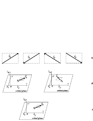
Figure 4: ’Similar’ initial velocity .

6 ’Similar’ trajectories

As a numerical application in Figure 5, there are given two ’similar’ trajectories for the binary system Earth-Moon ( $q=0.0121$ and $q^{\prime}=82.45$). The initial conditions are: $x_{0}=-0.2\;,\;\;y_{0}=-0.5\;,\;\;v_{0x}=-0.8\;,\;\;v_{0y}=-0.6\;,$ respectively $x_{0}^{\prime}=0.8\;,\;\;y_{0}^{\prime}=-0.5\;,\;\;v_{0x}^{\prime}=0.8\;,\;\;v_{0y}^{\prime}=0.6\;$. The time of integration is one Keplerian period.

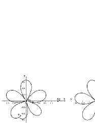
Figure 5: ’Similar’ trajectories .

In Figure 6, the ’similar’ trajectories for the same binary system, with initial conditions: $x_{0}=0.6\;,\;\;y_{0}=0.4\;,\;\;v_{0x}=0.5\;,\;\;v_{0y}=0\;,$ respectively $x_{0}^{\prime}=1.6\;,\;\;y_{0}^{\prime}=0.4\;,\;\;v_{0x}^{\prime}=-0.5\;,\;\;v_{0y}^{\prime}=0\;$ are presented. The time of integration is one Keplerian period. In Figure 7, there are given the ’similar’ trajectories for the same conditions as in Figure 6, but the time of integration is 200 Keplerian periods.

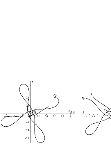
Figure 6: Others ’similar’ trajectories .

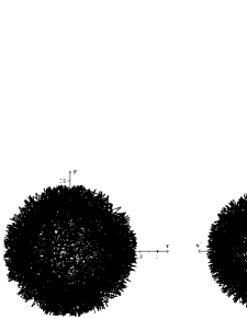
Figure 7: ’Similar’ trajectories for 200 Keplerian period time of integration.

7 The use of ’similar’ coordinate systems to demonstrate some analytical relations in the Roche geometry

We shall show now the consequence of ’similar’ coordinate system use on the equipotential curves (see Figure 8), and on the equilibrium points’ positions, in the frame of the Roche geometry.

From equations of motion (11)-(12) we obtain the equation of potential function:

$$\Psi(x,y)=\frac{1}{2}\left[\left(x-\frac{q}{1+q}\right)^{2}+y^{2}+\frac{2}{(1+q)r_{1}}+\frac{2q}{(1+q)r_{2}}\right]\;.$$

(We prefer to use this form, because in the second part of this paragraph we shall demonstrate some analytical relations of Seidov (2004), who denoted the expression in square brackets with $\psi(x,y)$, (see equation 21).) Similarly, from equations (14)-(15), the corresponding potential function is:

$$\Psi^{\prime}(x^{\prime},y^{\prime})=\frac{1}{2}\left[\left(x^{\prime}-\frac{q^{\prime}}{1+q^{\prime}}\right)^{2}+y^{\prime 2}+\frac{2}{(1+q^{\prime})r_{1}^{\prime}}+\frac{2q^{\prime}}{(1+q^{\prime})r_{2}^{\prime}}\right]\;.$$

In Figure 8 are represented the equipotential curves for a binary system characterized by the mass ratio $q=0.2$ (and by consequence $q^{\prime}=5$). Let us consider $L_{i}(x_{i},0)$, $i=\overline{1,5}$ the Lagrangian points. For the first Lagrangian point we obtained $x_{1}=0.65856$ and $x_{1}^{\prime}=0.34144$. The Jacobian constant ( (Szebehely, 1967) p.16 is $C_{1}=C_{1}^{\prime}=3.74897$. For the second Lagrangian point, $x_{2}=1.43808$ and $x_{2}^{\prime}=-0.43808$ and $C_{2}=C_{2}^{\prime}=3.53634$. For the third Lagrangian point, $x_{3}=-0.90250$ and $x_{3}^{\prime}=1.90250$ and $C_{3}=C_{3}^{\prime}=3.16504$. The points $L_{4}$ and $L_{5}$ form equilateral triangles with $S_{1}$ and $S_{2}$. The numerical results obtained above are normal, because $x^{\prime}=1-x$ (see equation(17)). In what concerne $C_{i}=C_{i}^{\prime}\;,\;\;i=\overline{1,3}$, the equalities are normal if we think at the physical meaning of the Jacobian constant. In Seidov (2004), there are obtained some analytical relations in the Roche geometry and one of them can be considered as an analytical demonstration of the relation $C_{i}=C_{i}^{\prime}\;,\;\;i=\overline{1,3}$. He obtained a very important correlation between the potential ($\psi$) and the mass ratio ($q$) on one side, and the Lagrangian points $L_{1}(x_{1},0)$ and $L_{2}(x_{2},0)$ on the other side, in the frame of the classical Roche model. The relations obtained by Seidov are:

$$\psi_{1}(q,x_{1})=\psi_{1}\left(1/q,1-x_{1}\right)\,,{}$$

$${}q(x_{i})\cdot q(1-x_{i})=1\,,\;\;i=\overline{1,2}.$$ (20)

The first relation of (20) correspond to $C_{i}=C_{i}^{\prime}\;,\;\;i=\overline{1,2}$ .

This paragraph will show an elegant and unitary proof for formulae (20), using the ‘similar’ coordinate systems. Using $q$, $q^{\prime}$, $r_{1}$, $r_{1}^{\prime}$, $r_{2}$, $r_{2}^{\prime}$ we will obtain these relations for $i=\overline{1,3}$ and we will expand the expressions concerning the potential for $i=\overline{4,5}$. So, the analytical relations of Seidov will be analyzed for all Lagrangian points, in a very easy manner.

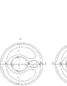
Figure 8: The ‘similar’ equipotential curves for the Roche model

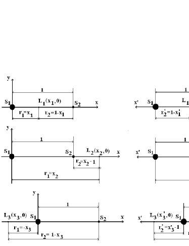
Figure 9: The ‘similar’ coordinate systems and the Lagrangian points $L_{1}$, $L_{2}$, and $L_{3}$.

The equation of the potential given in Seidov (2004) in the $(xS_{1}y)$ system is:

$$\psi(x,y) = \left(x-\frac{q}{1+q}\right)^{2}+y^{2}+{}$$ (21)

$${}\frac{2}{(1+q)r_{1}}+\frac{2q}{(1+q)r_{2}}$$

and if we use ’similar’ coordinate systems, the equation of the potential in $(x^{\prime}S_{2}y^{\prime})$ system becomes:

$$\psi^{\prime}(x^{\prime},y^{\prime}) = \left(x^{\prime}-\frac{q^{\prime}}{1+q^{\prime}}\right)^{2}+y^{\prime 2}{}$$ (22)

$${}+\frac{2}{(1+q^{\prime})r_{1}^{\prime}}+\frac{2q^{\prime}}{(1+q^{\prime})r_{2}^{\prime}}\;.$$

where

$$r_{1}=\sqrt{x^{2}+y^{2}}\,,\;\;r_{2}=\sqrt{(1-x)^{2}+y^{2}}\,,$$

$$r_{1}^{\prime}=\sqrt{x^{\prime 2}+y^{\prime 2}}\,,\;\;r_{2}^{\prime}=\sqrt{(1-x^{\prime})^{2}+y^{\prime 2}}\,.$$

$L_{i}(x_{i},0)$ being equilibrium points, we have $\partial\psi/\partial x_{i}=0$ and

$\partial\psi^{\prime}/\partial x_{i}^{\prime}=0$, $i=\overline{1,3}$ (see Figure 9). From these relations we obtain:

$$q(x_{1})=\frac{(1-x_{1})^{3}(1+x_{1}+x_{1}^{2})}{x_{1}^{3}(3-3x_{1}+x_{1}^{2})}\;,$$ (23)

$$q^{\prime}(x_{1}^{\prime})=\frac{(1-x_{1}^{\prime})^{3}(1+x_{1}^{\prime}+x_{1}^{\prime 2})}{x_{1}^{\prime 3}(3-3x_{1}^{\prime}+x_{1}^{\prime 2})}\;,$$ (24)

$$q(x_{2})=\frac{(x_{2}-1)^{3}(1+x_{2}+x_{2}^{2})}{x_{2}^{2}(2-x_{2})(1-x_{2}+x_{2}^{2})}\;,$$ (25)

$$q^{\prime}(x_{2}^{\prime})=-\frac{(1-x_{2}^{\prime})^{2}(x_{2}^{\prime 3}+1)}{x_{2}^{\prime 3}(3-3x_{2}^{\prime}+x_{2}^{\prime 2})}\;,$$ (26)

$$q(x_{3})=-\frac{(1-x_{3})^{2}(x_{3}^{3}+1)}{x_{3}^{3}(3-3x_{3}+x_{3}^{2})}\;,$$ (27)

$$q^{\prime}(x_{3}^{\prime})=\frac{(1-x_{3}^{\prime})^{2}(x_{3}^{\prime 3}-1)}{x_{3}^{\prime 2}(2-x_{3}^{\prime})(1-x_{3}^{\prime}+x_{3}^{\prime 2})}\;.$$ (28)

From (17) one can observe that $x_{i}^{\prime}=1-x_{i}\,,\;i=\overline{1,3}$, and therefore $q(x_{i})=\frac{1}{q^{\prime}(1-x_{i})}$, and $q(x_{i})\cdot q^{\prime}(1-x_{i})=1\;,i=\overline{1,3}$. These relations can be compared with the relations (20) given in Seidov (2004), for $i=\overline{1,2}$.

For $i=\overline{4,5}$ we have $L_{4}(\frac{1}{2},\frac{\sqrt{3}}{2})$, $L_{5}(\frac{1}{2},-\frac{\sqrt{3}}{2})$, (Roy, 1988; Murray, 2005), (the coordinates of $L_{4}$ and $L_{5}$ are independent of $q$), therefore $q$ is not a function of $x_{i}$, $i=\overline{4,5}$. Here $r_{1}=1=r_{2}$.

From (20) and (21), the potential corresponding to the Lagrangian points are:

$$\psi(q,x_{1}) = \left(x_{1}-\frac{q}{1+q}\right)^{2}+{}$$ (29)

$${}\frac{2}{(1+q)x_{1}}+\frac{2q}{(1+q)(1-x_{1})}\;,$$

$$\psi^{\prime}(q^{\prime},x_{1}^{\prime}) = \left(x_{1}^{\prime}-\frac{q^{\prime}}{1+q^{\prime}}\right)^{2}+{}$$ (30)

$${}\frac{2}{(1+q^{\prime})x_{1}^{\prime}}+\frac{2q^{\prime}}{(1+q^{\prime})(1-x_{1}^{\prime})}\;,$$

$$\psi(q,x_{2}) = \left(x_{2}-\frac{q}{1+q}\right)^{2}+{}$$ (31)

$${}\frac{2}{(1+q)x_{2}}-\frac{2q}{(1+q)(1-x_{2})}\;,$$

$$\psi^{\prime}(q^{\prime},x_{2}^{\prime}) = \left(x_{2}^{\prime}-\frac{q^{\prime}}{1+q^{\prime}}\right)^{2}-{}$$ (32)

$${}\frac{2}{(1+q^{\prime})x_{2}^{\prime}}+\frac{2q^{\prime}}{(1+q^{\prime})(1-x_{2}^{\prime})}\;,$$

$$\psi(q,x_{3}) = \left(x_{3}-\frac{q}{1+q}\right)^{2}-{}$$ (33)

$${}\frac{2}{(1+q)x_{3}}+\frac{2q}{(1+q)(1-x_{3})}\;,$$

$$\psi^{\prime}(q^{\prime},x_{3}^{\prime}) = \left(x_{3}^{\prime}-\frac{q^{\prime}}{1+q^{\prime}}\right)^{2}+{}$$ (34)

$${}\frac{2}{(1+q^{\prime})x_{3}^{\prime}}-\frac{2q^{\prime}}{(1+q^{\prime})(1-x_{3}^{\prime})}\;.$$

Using the equations: $x_{i}^{\prime}=1-x_{i}$, and $q^{\prime}=1/q$ we obtain:

$$\psi(q,x_{i})=\psi^{\prime}(1/q,1-x_{i})\;,\qquad i=\overline{1,3}\;.$$

These relations can be compared with relations (20) given in Seidov (2004) for $i=\overline{1,2}$.

For $L_{4}(\frac{1}{2},\frac{\sqrt{3}}{2})$, using the equations (20) and (21) we obtain

$$\psi(q)=\frac{3+5q+3q^{2}}{(1+q)^{2}}\;,\qquad\psi^{\prime}(q^{\prime})=\frac{3+5q^{\prime}+3q^{\prime 2}}{(1+q^{\prime})^{2}}$$

and because $q^{\prime}=1/q$, for $L_{4}$ we obtain $\psi(q)=\psi^{\prime}(1/q)$.

For $L_{5}(\frac{1}{2},-\frac{\sqrt{3}}{2})$ the same equation is obtained.

From equations (23)-(28) and (29)-(34) we obtain analytical formulae for the potential as a function of Lagrangian point positions:

$$\psi(x_{1})=-\frac{4x_{1}^{8}-16x_{1}^{7}+14x_{1}^{6}+14x_{1}^{5}-41x_{1}^{4}+40x_{1}^{3}-27x_{1}^{2}+12x_{1}-3}{(x_{1}^{4}-2x_{1}^{3}-x_{1}^{2}+2x_{1}-1)^{2}}$$

$$\psi(x_{2})=\frac{4x_{2}^{7}-14x_{2}^{6}+18x_{2}^{5}+9x_{2}^{4}-36x_{2}^{3}+27x_{2}^{2}-4x_{2}-1}{(x_{2}^{4}-2x_{2}^{3}-x_{2}^{2}+2x_{2}-1)^{2}}$$

$$\psi(x_{3})=-\frac{4x_{3}^{7}-14x_{3}^{6}+18x_{3}^{5}-29x_{3}^{4}+40x_{3}^{3}-27x_{3}^{2}+12x_{3}-3}{(x_{3}^{4}-2x_{3}^{3}+x_{3}^{2}-2x_{3}+1)^{2}}$$

$$\psi^{\prime}(x_{1}^{\prime})=-\frac{4x_{1}^{\prime}\,{}^{8}-16x_{1}^{\prime}\,{}^{7}+14x_{1}^{\prime}\,{}^{6}+14x_{1}^{\prime}\,{}^{5}-41x_{1}^{\prime}\,{}^{4}+40x_{1}^{\prime}\,{}^{3}-27x_{1}^{\prime}\,{}^{2}+12x_{1}^{\prime}\,-3}{(x_{1}^{\prime}\,{}^{4}-2x_{1}^{\prime}\,{}^{3}-x_{1}^{\prime}\,{}^{2}+2x_{1}^{\prime}\,-1)^{2}}$$

$$\psi^{\prime}(x_{2}^{\prime})=-\frac{4x_{2}^{\prime}\,{}^{7}-14x_{2}^{\prime}\,{}^{6}+18x_{2}^{\prime}\,{}^{5}-29x_{2}^{\prime}\,{}^{4}+40x_{2}^{\prime}\,{}^{3}-27x_{2}^{\prime}\,{}^{2}+12x_{2}^{\prime}\,-3}{(x_{2}^{\prime}\,{}^{4}-2x_{2}^{\prime}\,{}^{3}+x_{2}^{\prime}\,{}^{2}-2x_{2}^{\prime}\,+1)^{2}}$$

$$\psi^{\prime}(x_{3}^{\prime})=\frac{4x_{3}^{\prime}\,7-14x_{3}^{\prime}\,{}^{6}+18x_{3}^{\prime}\,{}^{5}+9x_{3}^{\prime}\,{}^{4}-36x_{3}^{\prime}\,{}^{3}+27x_{3}^{\prime}\,{}^{2}-4x_{3}^{\prime}\,-1}{x_{3}^{\prime}\,{}^{4}-2x_{3}^{\prime}\,{}^{3}+x_{3}^{\prime}\,{}^{2}+2x_{3}^{\prime}\,-1}$$

The equation for $\psi(x_{2})$ is obtained also by Seidov (see equation (9) in Seidov (2004)).

8 Conclusion

The ’similarity’ relation defined in section 2 belongs to equivalence relations’ family. For the time being it has only a theoretical value, completing classical method of study of the restricted three-body problem (see sections 4, 5, 6), and allowing for a more elegant demonstration of some analytical relations from the geometry of the Roche model (section 7). The use of ’similar’ coordinate systems imposes the typical definitions of mass ratio, of distances from the test particle to the components of the binary system, and of initial conditions necessary to integrate the differential equations of motion. The ’similar’ trajectories are not like-wise, but have a similar topology.

The use of ‘similar’ coordinate systems helped us to create an elegant and easy proof for the analytical relations obtained by Seidov (2004). To close the circle, we have completed these relations by analyzing the problem of mass ratio and potential, as function of Lagrangian point positions for all five Lagrangian points. So, the use of ’similar’ coordinate systems in the restricted three-body problem enable us to complete the study of the Roche geometry with some new elements.

References

- Huang (1967) Huang, S. Sh., in ”Modern Astrophysics. A memorial to Otto Struve”, ed. M. Hack, Gauthier-Villars, Paris, Gordon and Breach, New York, p.211 (1967)
- Kitamura (1970) Kitamura, M., Ap & SS, 7, 272 (1970)
- Kopal (1989) Kopal, Z., The Roche Problem, Dordrecht: Kluwer (1989)
- Kopal (1978) Kopal, Z., Dynamics of Close Binary Systems, Dordrecht: Reidel (1978)
- Kruszewski (1963) Kruszewski, A., Acta Astron., 13, 106 (1963)
- Moulton (1923) Moulton, F. R., An introduction to celestial mechanics, Second Edition, The Macmillan Company, New York (1923)
- Murray (2005) Murray, C. D., & Dermott, S. F., Solar System Dynamics, Cambridge: Cambridge University Press (2005)
- Roy (1988) Roy, A. E., Orbital Motion, Bristol: Adam Hilger (1988)
- Seidov (2004) Seidov, Z. F., ApJ, 603, 283 (2004)
- Szebehely (1967) Szebehely, V., Theory of Orbits, New York: Academic Press (1967)