Anomalous diffusion in systems driven by the stable Lévy noise with a finite noise relaxation time and inertia

Abstract

Dynamical systems driven by a general Lévy stable noise are considered. The inertia is included and the noise, represented by a generalised Ornstein-Uhlenbeck process, has a finite relaxation time. A general linear problem (the additive noise) is solved: the resulting distribution converges with time to the distribution for the white-noise, massless case. Moreover, a multiplicative noise is discussed. It can make the distribution steeper and the variance, which is finite, depends sublinearly on time (subdiffusion). For a small mass, a white-noise limit corresponds to the Stratonovich interpretation. On the other hand, the distribution tails agree with the Itô interpretation if the inertia is very large. An escape time from the potential well is calculated.

I Introduction

A prominent feature of the stable Lévy processes is the existence of algebraic, long tails of the probability distributions of the form $|x|^{-\alpha-1}$, where $0<\alpha<2$ is a stability index. As a consequence, the moments, in particular the variance, are divergent. The diffusion process in such systems is called an ”accelerated diffusion” and the relative transport rate may be described by a time-dependence of the fractional moments instead of the variance. However, there are indications that in some physical problems the distribution tails fall faster than for the pure Lévy flight. In the field of the economic research, the indexes 2.5 – 4 were observed in financial data sta ; it has been suggested that such values of the index arise when the trading behaviour is performed in an optimal way gab . The probability distributions of the hydraulic conductivity in the porous media seem to obey the power law with the index 3.5, while the atmospheric turbulence studies yield even larger index for the wind field sche . Such slowly falling algebraic tails are predicted by the Langevin equation with the Lévy stable noise – in a sense of the stationary solution – when one introduces an appropriate deterministic potential. It has been demonstrated by Chechkin et al. che that the stationary distribution tails of the form $x^{-\alpha-2m-1}$ result from the potential $\sim x^{2m+2}$. Also temporal characteristics of the system may influence the asymptotic shape of the distribution. This happens if, for a jumping process, long jumps are penalised by a short waiting time. The finite variance is observed for such jumping processes as the Lévy walk kla and the kangaroo process with a Lévy distributed jumping size srkan .

The Lévy stable processes are often connected with complex phenomena for which the power-law shape of the distribution tails newm is typical, as well as a complicated structure of the medium. It is the case for the porous media, plasmas and fractal (multifractal) structures sche ; park . Therefore, a nonhomogeneity must often be taken into account in a dynamical description, both as a deterministic potential and as a multiplicative noise. Descriptions of the diffusion on fractals involve the variable, power-law diffusion coefficient osh ; met4 . Also the other topologically complicated systems with long jumps, the folded polymers, require a variable diffusion coefficient to describe the transport bro . Moreover, formalisms with the multiplicative Lévy noise can describe the second order phase transitions manor and the dynamics of two competing species cogn . A nonlinearity of the Langevin equation makes the stochastic process different from the pure Lévy motion. In particular, variance may be finite for a system driven by the multiplicative Lévy noise sro1 . Generally, the variance rises not only linearly with time but also faster or slower than that, i.e. the diffusion may be anomalous. In the case of Ref.sro1 , motion is subdiffusive. The above approach includes the white noise. However, a Markovian description of a realistic system is an idealisation, valid only if the time scale of fast variables is short, compared to the time scale of the process variable. A procedure of the fast variables elimination produces correlations: they are present even if the original system is Markovian hae . It has been demonstrated for the Gaussian noise that characteristic time scales of the fast variables are important even if the variables themselves are eliminated ter ; this finding suggests using a coloured noise in a stochastic description rather than the white noise. Effects related to the correlations are important, for example, for such problems as fluctuations of a dye laser light sho and a narrowing of the magnetic resonance lines kub . Importance of the finite correlation time for noise-induced phase transitions was emphasised in Ref.mang ; an increase of that time favours disorder and prevents the formation of an ordered state. Introducing the white noise as a limit of the finite correlation time means that the stochastic integral should be interpreted in a Stratonovich sense won . On the other hand, effects of the finite inertia should be taken into account. If the relaxation time associated with the inertia is large compared to the correlation time, the Itô interpretation comes into play kup . That effect of the inertia, opposite to the correlations, was demonstrated in Ref.san : it modifies the front propagation by suppressing the external multiplicative, white noise influence on the velocity of fronts.

The Itô-Stratonovich dilemma becomes especially interesting for $\alpha<2$ since then – when we consider the white Lévy noise and neglect the inertia – the very existence of the variance depends on the particular interpretation of the stochastic integral. This problem is important for the diffusion since the infinite variance, which means the infinite propagation speed, is unphysical in most cases. How do the finite noise relaxation time and the inertia modify slope of the distribution? We address this question in the present paper and discuss consequences for the diffusion. In Sec.II a linear problem involving the additive noise is considered. Sec.III is devoted to the multiplicative noise; both limiting, analytically solvable cases and numerical solutions are discussed. Moreover, the escape time from a potential well is calculated. Results are summarised in Sec.IV.

II Additive noise

We consider a linear problem which is defined by the following system of the Langevin equations for $x$, $v$ and $\xi$:

$$m\dot{v}(t) = f_{0}-\beta v(t)-\lambda x+\gamma\xi(t)$$

$$\dot{x}(t) = v(t)$$

$$d\xi(t) = -\gamma\xi(t)dt+dL(t),$$ (1)

where $\beta$ is a damping coefficient. The stochastic force, $dL(t)$, is the symmetric and stable Lévy process, characterised by the stability index $\alpha\in(0,2]$. Special cases of the system (II) were considered by several authors. The velocity distribution for the white noise without a potential was obtained in Ref.west , the linear force case was discussed in Ref.jes and the white noise case with the inertia for $\alpha=1$ in Ref.garb . Moreover, the asymmetric Lévy distribution was introduced in Ref.yan . On the other hand, stochastic collision models may lead to the Lévy statistics. The Fokker-Planck equation with the additive noise predicts, in the limit of small mass, an equilibrium in the form of the Lévy distribution barkai . The case $\alpha=2$ corresponds to the normal distribution. Then the third equation (II) describes the standard Ornstein-Uhlenbeck process with the covariance

$$\langle\xi(t)\xi(0)\rangle=\langle\xi^{2}(0)\rangle{\hbox{e}}^{-\gamma t};$$ (2)

therefore $\gamma$ determines a correlation time, $1/\gamma$. A generalisation of the Ornstein-Uhlenbeck process for $\alpha<2$ implies an infinite covariance for any time. However, the parameter $\gamma$ can still estimate the noise relaxation time. One can modify the covariance definition emb ; elia to get a convergent quantity which behaves with time similar to Eq.(2). On the other hand, the covariance becomes finite when one introduces a truncation of the Lévy distribution act . Properties of such a dynamical system are similar to the system without the truncation for an arbitrarily large time man and the parameter $\gamma$ measures the correlation time. Values of the process $dL(t)$ are given by the characteristic function ${\widetilde{p}}(k)=\exp(-K^{\alpha}|k|^{\alpha})$ $(K>0)$. The fractional Fokker-Planck equation

$$\frac{\partial}{\partial t}p=-v\frac{\partial}{\partial x}p-\frac{1}{m}(f_{0}-\beta v-\lambda x+\gamma\xi)\frac{\partial}{\partial v}p+\gamma\frac{\partial}{\partial\xi}(\xi p)+\frac{\beta}{m}p+K^{\alpha}\frac{\partial^{\alpha}}{\partial|\xi|^{\alpha}}p$$ (3)

determines the probability density distribution $p(x,v,\xi;t|x_{0},v_{0},\xi_{0};0)$ and the fractional Weyl derivative is defined by its Fourier transform, ${\cal F}[\frac{\partial^{\alpha}}{\partial|x|^{\alpha}}f(x)]=-|k|^{\alpha}{\widetilde{f}}(k)$. We will evaluate the density of $x$, $p(x,t)$, directly from the stochastic equation (II). We restrict our analysis to the case of a relatively weak potential; more precisely: let $\beta^{2}/m^{2}-4\lambda/m\equiv\Delta^{2}>0$. First, we need to evaluate the stochastic trajectory $x(t)$. The solution of Eq.(II) produces the result

$$x(t)=f_{1}+\int_{0}^{t}f_{2}(t^{\prime})L(t^{\prime})dt^{\prime},$$ (4)

where

$$f_{1}=\frac{2v_{0}}{\Delta}{\hbox{e}}^{-\beta t/2m}\sinh\frac{\Delta}{2}t+\frac{2f_{0}}{m\Delta}\left[\frac{m\Delta}{2\lambda}+\exp(-\frac{1}{2}\frac{\beta}{m}t)\left(\frac{\exp(-\frac{\Delta}{2}t)}{\beta/m+\Delta}-\frac{\exp(\frac{\Delta}{2}t)}{\beta/m-\Delta}\right)\right]$$ (5)

and

$$f_{2}(t^{\prime})=\frac{\gamma}{m\Delta}{\hbox{e}}^{-\gamma(t-t^{\prime})}\left[\frac{\exp[(\gamma-\frac{\beta}{2m}+\frac{\Delta}{2})(t-t^{\prime})]}{\gamma-\beta/2m+\Delta/2}-\frac{\exp[(\gamma-\frac{\beta}{2m}-\frac{\Delta}{2})(t-t^{\prime})]}{\gamma-\beta/2m-\Delta/2}+\frac{m\Delta}{m\gamma^{2}-\gamma\beta+\lambda}\right].$$ (6)

Two simple special cases are distinguished. In the absence of inertia ($m=0$), we have an adiabatic problem of the particle subjected to the linear force and the coloured Lévy noise. Then Eq.(II) yields

$$f_{2}(t^{\prime})=\frac{\gamma}{\lambda-\beta\gamma}\left({\hbox{e}}^{\lambda t/\beta-\gamma(t-t^{\prime})}-{\hbox{e}}^{\lambda t^{\prime}/\beta}\right).$$ (7)

Secondly, for the case of a free-particle ($\lambda=0$) we obtain

$$f_{2}(t^{\prime})=\frac{1}{\beta}+\left(\frac{1}{\gamma-\beta/m}-\frac{1}{\beta}\right){\hbox{e}}^{-\gamma(t-t^{\prime})}-\frac{1}{\gamma-\beta/m}{\hbox{e}}^{-\beta(t-t^{\prime})/m}.$$ (8)

The characteristic function of $p(x,t)$ directly follows from Eq.(6) doo ; west :

$${\widetilde{p}}(k,t)=\langle{\hbox{e}}^{ikx(t)}\rangle={\hbox{e}}^{ikf_{1}}\langle\exp(ik\int_{0}^{t}f_{2}(t^{\prime})dt^{\prime})\rangle={\hbox{e}}^{ikf_{1}}\exp\left(-K^{\alpha}|k|^{\alpha}\int_{0}^{t}|f_{2}(t^{\prime})|^{\alpha}dt^{\prime}\right).$$ (9)

Eq.(9) implies the Lévy distribution with the same stability index as the driving noise $L$ and a translation parameter which coincides with $f_{1}$ and for large time equals either $f_{0}/\lambda$ ($\lambda\neq 0$) or $f_{0}(t-m/\beta)$ ($\lambda=0$). Since the dependence of the density distribution on $f_{0}$ is trivial, we assume in the following $f_{0}=0$ and $v_{0}=0$. Then the distribution is symmetric for any time. The inverse Fourier transform can be conveniently expressed in a form of the Fox function mat ; sri :

$$p(x,t)=Nf(t)H_{2,2}^{1,1}\left[f(t)|x|\left|\begin{array}[]{c}(1-1/\alpha,1/\alpha),(1/2,1/2)\\ \\ (0,1),(1/2,1/2)\end{array}\right.\right],$$ (13)

where $f(t)=K^{\alpha}\int_{0}^{t}|f_{2}(t^{\prime})|^{\alpha}dt^{\prime}$. By introducing a new variable $\tau=t-t^{\prime}$ we have $f(t)=K^{\alpha}(\int_{0}^{T}+\int_{T}^{t})$ and the exponentials in the second integral can be dropped for any $T\gg 1$. Therefore $f(t)=t/\beta+$const for large times. Since $p(x,t)\sim|x|^{-1-\alpha}$ for $|x|\to\infty$, variance and all higher moments of the distribution (13) are divergent, as well as the average if $\alpha\leq 1$. A relative expansion rate can be quantified by the fractional moments of the order $\delta<\alpha$, $\langle|x|^{\delta}\rangle(t)$; they are given by the Mellin transform from the Fox function kla . The final expression reads

$$\langle|x|^{\delta}\rangle=\frac{2}{\alpha}f(t)^{\delta/\alpha}\frac{\Gamma(-\delta/\alpha)\Gamma(1+\delta)}{\Gamma(-\delta/2)\Gamma(1+\delta/2)}.$$ (14)

Consequently, in the limit of large $t$ the fractional moments decrease with the damping coefficient $\beta$ and the expansion rate is large for small $\alpha$.

As an example, let us consider the case $\alpha=1$ for which results take the transparent form. This particular value of the stability parameter corresponds to the well-known Cauchy distribution; it was considered in Ref.garb for the white noise. For $\gamma>\beta/m$, a straightforward calculation yields the expression for the apparent width of the distribution $p(x,t)$:

$$f(t)=\frac{t}{\beta}-\frac{1+m}{\gamma\beta}-\frac{1}{\gamma}\left(\frac{1}{\gamma-\beta/m}-\frac{1}{\beta}\right){\hbox{e}}^{-\gamma t}+\frac{m}{\beta}\frac{1}{\gamma-\beta/m}{\hbox{e}}^{-\beta t/m}.$$ (15)

In the limit of the large time, inertia and noise relaxation time are responsible for a time-shift which is negative and rises with $m$ and $1/\gamma$.

III Multiplicative noise

By introducing a multiplicative noise we take into account that the influence of the random component of the dynamics depends on the dynamics itself. The one-dimensional case is given by the Langevin equation

$$m\dot{v}(t) = -\partial V(x)/\partial x-\beta v(t)+\gamma G(x)\xi(t)$$

$$\dot{x}(t) = v(t)$$

$$d\xi(t) = -\gamma\xi(t)dt+dL(t).$$ (16)

In the following we assume the noise intensity in the algebraic form, $G(x)=|x|^{-\theta/\alpha}$ $(\alpha+\theta>0)$.

The simplest problem involves the white noise ($\gamma\to\infty$) and neglects the inertia. The latter condition means that mass is small compared to the damping parameter $\beta$ and the strength of the noise. The case of the normal distribution, $\alpha=2$, is well-known schen ; vkam ; gra . A stochastic integral in the Langevin equation is not completely determined for the uncorrelated noise, since it is not clear whether the dynamical variable in the function $G(x)$ should be evaluated at the time before the noise acts, after that, or somewhere in between. Two interpretations are of particular importance. In the Itô interpretation, the $i$’s component of the discretized stochastic integral is $G[x(t_{i-1})][\xi(t_{i})-\xi(t_{i-1})]$, whereas the Stratonovich interpretation includes both the beginning and the end of each interval: $G\{[x(t_{i-1})+x(t_{i})]/2\}[\xi(t_{i})-\xi(t_{i-1})]$. Both assumptions result in a different Fokker-Planck equation but a difference resolves itself solely to a drift term (the spurious drift) which can be eliminated by an appropriate modification of the deterministic potential. For this reason, a physical relevance of the Itô-Stratonovich dilemma is disputed vkam . Nevertheless, physical implications of both interpretations may be different. For example, phase transitions due to instabilities of the disordered phase in the framework of the Ginzburg-Landau model take place only for the Stratonovich interpretation car . Rules of the ordinary calculus are valid in the Stratonovich formalism, in contrast to the Itô interpretation.

The meaning of both interpretations becomes more transparent when we take into account the finite correlations and inertia. First of all, the memory effects favour the Stratonovich interpretation since it constitutes the white-noise limit of the correlated processes won . Inertia acts in the opposite direction. It was demonstrated kup – by the estimation of the velocity moments and using the Itô formula – that if the inertia relaxation time goes to zero faster than the noise correlation time, the Stratonovich interpretation is valid. The opposite limit produces the Itô result. If both time scales are comparable, neither of the above interpretations is valid. We will demonstrate that similar conclusions can be drawn for the general Lévy stable processes. However, for $\alpha<2$ methods of Ref.kup cannot be applied since the moments are divergent and the Itô formula is unknown.

We take into account only Itô and Stratonovich interpretations of the stochastic integral. The Itô interpretation applies, beside the systems with large mass, to discrete problems; it is commonly used in the perturbation theory gar . However, there are indications that other interpretations are also important. For example, it was recently experimentally demonstrated that description of the Brownian motion in the presence of gravitational and electrostatic forces requires a backward integral (anti-Itô interpretation) volpe .

III.1 White-noise case without the inertia

To study a diffusion process, we consider a free particle, $V(x)=0$. In the limit $m\to 0$ and $\gamma\to\infty$, Eq.(III) becomes a single Langevin equation of the first order:

$$dx(t)=|x(t)|^{-\theta/\alpha}dL(t),$$ (17)

where, for simplicity, we assumed $\beta=1$. In the Itô interpretation it corresponds to the Fokker-Planck equation sche

$$\frac{\partial}{\partial t}p_{I}(x,t)=K^{\alpha}\frac{\partial^{\alpha}}{\partial|x|^{\alpha}}[|x|^{-\theta}p_{I}(x,t)],$$ (18)

which differs from the equation for the additive noise by an algebraic term under the fractional derivative. This particular form of the multiplicative factor suggests simple scaling properties and a possible similarity of the solution to Eq.(13). Indeed, an asymptotic solution of Eq.(18) can be found in the form $a(t)H_{2,2}^{1,1}[a(t)x]$. The procedure is the following physa . First, we insert the above expression to the Langevin equation and take the Fourier transform, which also has a form of the Fox function but of a higher order. Expansion of the Fox functions in powers of $k$ and neglecting the terms of the order $|k|^{2\alpha+\theta}$ and higher yields a simple differential equation for the function $a(t)$ and allows us to determine some Fox function coefficients. Finally, we obtain the solution

$$p_{I}(x,t)=Na(t)H_{2,2}^{1,1}\left[a(t)|x|\left|\begin{array}[]{c}(1-\frac{1-\theta}{\alpha+\theta},\frac{1}{\alpha+\theta}),(a_{2},A_{2})\\ \\ (b_{1},B_{1}),(1-\frac{1-\theta}{2+\theta},\frac{1}{2+\theta})\end{array}\right.\right],$$ (22)

where $a(t)\sim t^{-1/(\alpha+\theta)}$ and the coefficients $(a_{2},A_{2})$ and $(b_{1},B_{1})$ are arbitrary. The asymptotic form of the solution is the same as for the driving noise,

$$p_{I}(x,t)\sim|x|^{-1-\alpha}.$$ (23)

Therefore, for the Itô interpretation the variance is always divergent which implies accelerated diffusion. Fractional moments can be evaluated similarly to the additive noise case; a straightforward calculation yields

$$\langle|x|^{\delta}\rangle\sim t^{\delta/(\alpha+\theta)}.$$ (24)

The multiplicative noise parameter $\theta$ can both strengthen ($\theta<0$) and weaken ($\theta>0$) the time-dependence of $\langle|x|^{\delta}\rangle$, compared to the case of the additive noise. The undetermined coefficients do not influence the functional dependences. The same method of solution can be applied in the presence of the linear deterministic force $F(x)=-\lambda x$ sro1 .

Results for the Stratonovich interpretation are qualitatively different since the decline of the noise intensity with $x$ may compensate the effect of the long jumps. The technical advantage of this interpretation, for one-dimensional systems, consists in a possibility of applying rules of the ordinary calculus. This property is strict for $\alpha=2$ gar . In the general case, the noise distribution must be truncated, a requirement that is obvious for the linear systems sro2 . However, it was numerically demonstrated that in practice cases with the distribution without any cut-off also comply with rules of the ordinary calculus if the system is nonlinear sro1 ; sro2 . Then we may define a new variable,

$$y(x)=\frac{\alpha}{K(\alpha+\theta)}|x|^{1+\theta/\alpha}\hbox{sgn}(x),$$ (25)

which transforms Eq.(17) to the equation with the additive noise. The asymptotic form of the solution sro1

$$p_{S}(x,t)\sim t^{\alpha/(\alpha+\theta)}|x|^{-1-\alpha-\theta}~{}~{}~{}~{}(|x|\to\infty)$$ (26)

implies that variance may be convergent. It takes the form $\langle x^{2}\rangle\sim t^{2/(\alpha+\theta)}$ on the condition $\alpha+\theta>2$. Therefore, diffusion is either anomalously weak – if the above condition is satisfied – or accelerated uwa .

III.2 General case

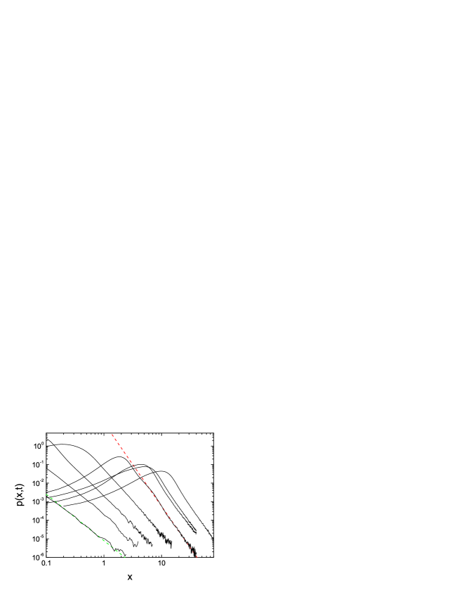
Figure 1: (Colour online) Probability density distributions at $t=1$ for $\alpha=1.5$, $\theta=2$, $\gamma=100$ and $\beta=1$. The curves correspond to the following values of $m$ (from left to right): $5\times 10^{5}$, $5\times 10^{4}$, $10^{4}$, $10^{3}$, 0.01, 0.1, 10, 1. The red dashed line marks the depedence $x^{-4.5}$ and the green dashed line (at the left side) the dependence $x^{-2.5}$. Each curve was obtained by averaging over $10^{8}$ trajectories.

First let us consider the overdamped limit (the adiabatic approximation) by putting $m=0$ in Eq.(III). Equations take the form

$$\dot{x}(t) = \frac{\gamma}{\beta}|x|^{-\theta/\alpha}\xi(t)$$

$$d\xi(t) = -\gamma\xi(t)dt+dL(t).$$ (27)

After transformation of the process variable according to Eq.(25), we obtain a linear equation with the additive noise. Its solution reads $y(t)=\int_{0}^{t}f_{2}(t^{\prime})L(t^{\prime})dt^{\prime}$, where $f_{2}(t^{\prime})=(1-{\hbox{e}}^{-\gamma(t-t^{\prime})})/\beta$, and the density distribution of $y$ has the Lévy form, Eq.(13). Transformation to the variable $x$ yields the final result:

$$p(x,t)=\frac{\alpha+\theta}{\alpha^{2}|x|}H_{2,2}^{1,1}\left[\frac{|x|^{1+\theta/\alpha}}{K(1+\theta/\alpha)f(t)^{1/\alpha}}\left|\begin{array}[]{l}(1,1/\alpha),(1,1/2)\\ \\ (1,1),(1,1/2)\end{array}\right.\right],$$ (31)

where $f(t)=K^{\alpha}\int_{0}^{t}|f_{2}(t^{\prime})|^{\alpha}dt^{\prime}$. The expansion of Eq.(31) in the fractional powers of $|x|^{-1}$ yields an approximation of the solution for large $|x|$ and the first term is of the form

$$p(x,t)\sim f(t)^{\alpha/(\alpha+\theta)}|x|^{-1-\alpha-\theta}.$$ (32)

If $\alpha+\theta>2$, the variance is convergent and it can be exactly evaluated by using properties of the Fox functions, in particular, an expression for the Mellin transform. A straightforward calculation yields

$$\langle x^{2}\rangle=-\frac{2}{\pi\alpha}\left[K(\frac{\theta}{\alpha}+1)\right]^{2\alpha/(\alpha+\theta)}\Gamma\left(-\frac{2}{\alpha+\theta}\right)\Gamma\left(1+\frac{2\alpha}{\alpha+\theta}\right)\sin\left(\frac{\pi\alpha}{\alpha+\theta}\right)f(t)^{2/(\alpha+\theta)}.$$ (33)

Eq.(31) converges to the white-noise solution in the Stratonovich interpretation for any noise relaxation parameter $\gamma$ if time is large or, for any time, if $\gamma\to\infty$.

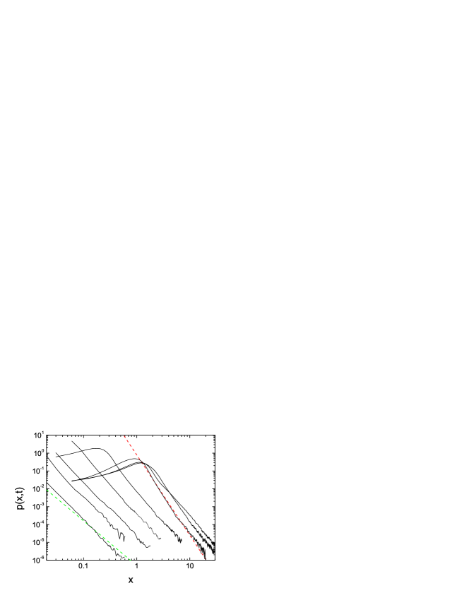
Figure 2: (Colour online) Same as Fig.1 but for $\gamma=1$. The following values of $m$ are presented (from left to right): $5\times 10^{5}$, $5\times 10^{4}$, $10^{4}$, $10^{3}$, $10^{2}$, 0.01, 0.1, 1.

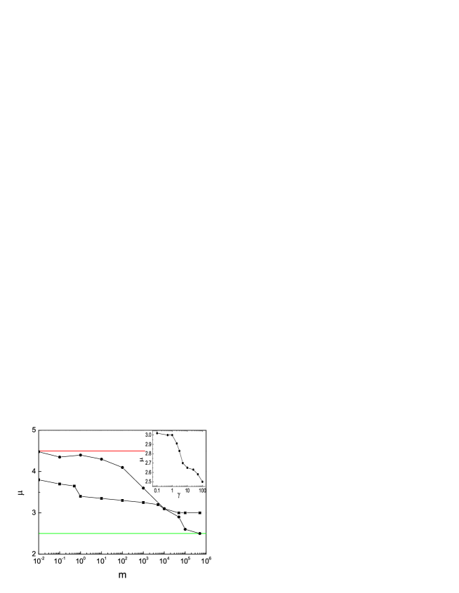
Figure 3: (Colour online) Slopes of the tails, $|x|^{-\mu}$, of $p(x,t)$ at $t=1$ for $\alpha=1.5$, $\theta=2$ and $\beta=1$, as a function of $m$. Two cases are presented: $\gamma=100$ (points) and $\gamma=1$ (squares). The limiting values, $\mu_{S}$ and $\mu_{I}$, are marked by the horizontal lines. Inset: $\mu$ as a function of $\gamma$ for $m=5\times 10^{5}$.

Distributions for arbitrary $\gamma$ and $m$ have been obtained by a numerical integration of the stochastic equations, Eq.(III). For that purpose, a second order difference approximation, called a Störmer method dahl , was applied to the first two equations. Since the resulting difference equations are implicit, the parabolic interpolation scheme was applied at each step ral . The third equation was integrated by an Euler method and the noise term in the $i$-step was represented by $\tau^{1/\alpha}L_{i}$, where $\tau$ was a time step wer . We will demonstrate how the asymptotic shape of the distribution, for a given time, depends on $m$ and $\gamma$. Another quantity of interest is a time dependence of the variance.

Fig.1 presents the probability density distributions as a function of the particle mass in the limit of the white noise at $t=1$. The distributions widen with $m$ up to $m=1$ but then the trend goes into reverse. For the large mass the distributions have a form of the delta function accompanied by a little tail. The tails are algebraic, $\sim|x|^{-\mu}$, and the slope $\mu$ diminishes with the mass. Two limiting values, $\mu_{S}=\alpha+\theta+1$ and $\mu_{I}=\alpha+1$, correspond to the Stratonovich, Eq.(26), and Itô, Eq.(23), interpretations, respectively. The distributions for the case of the finite noise relaxation time ($\gamma=1$) are presented in Fig.2. They are similar to those for the white noise but the limiting slopes are not yet reached at $t=1$. Slopes for all cases are put together in Fig.3. The dependence $\mu(m)$ is flat for $\gamma=1$ whereas for the white-noise case large values of $\mu$ dominate and there is a rapid transition to $\mu_{I}$. Variance is finite ($\mu>3$) except for the very large $m$. This case is separately presented in Fig.3: $\mu$ rises with the noise relaxation time from the Itô value for the white noise, $\mu=2.5$, to $\mu=3$, where it saturates.

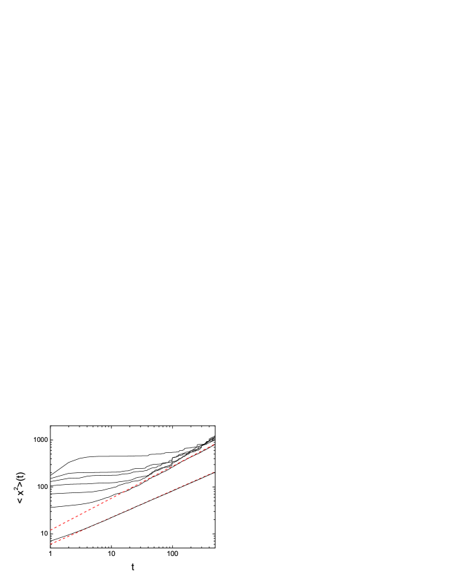
Figure 4: (Colour online) Variance as a function of time for $\alpha=1.5$, $\theta=2$, $\gamma=100$ and $\beta=1$. The curves correspond to the following values of $m$ (from bottom to top): 0.01, 0.1, 0.2, 0.3, 0.4, 0.5, 1. The red dashed lines mark the dependence $t^{0.57}$ (lower) and $t^{0.68}$ (upper).

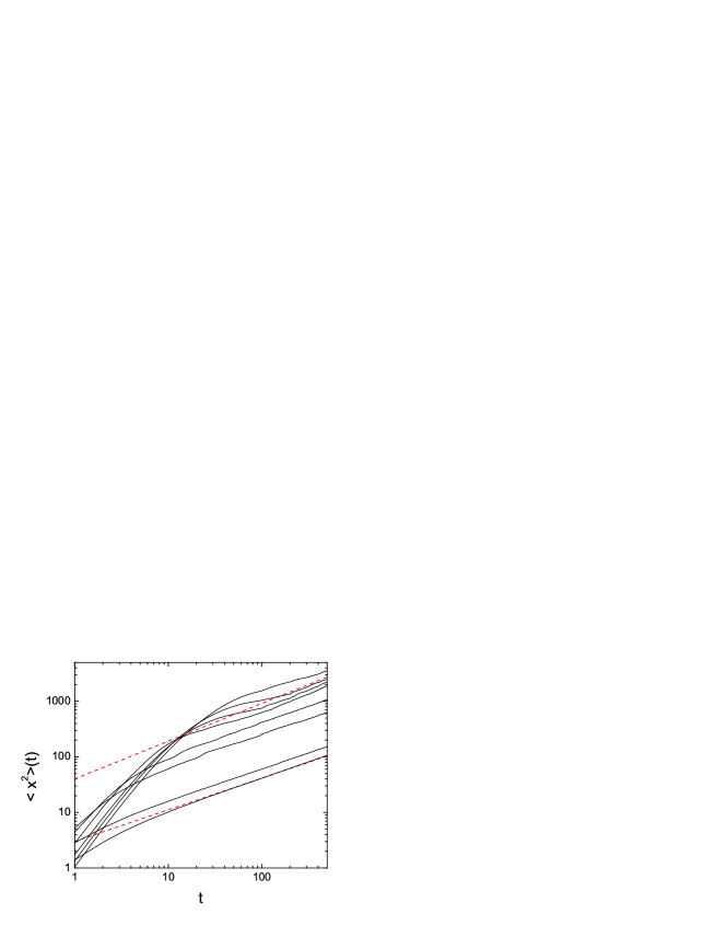
Figure 5: (Colour online) The same as Fig.4 but for $\gamma=1$. The curves correspond to the following values of $m$ (from bottom to top on the right side): 0.01, 0.1, 1, 2, 5, 10, 15, 20.

Diffusion properties of the system are determined by a long-time behaviour of the variance. The case corresponding to the short noise relaxation time is presented in Fig.4. If $m$ is very small, the variance assumes the form $\langle x^{2}\rangle\sim t^{2/(\alpha+\theta)}$ for the large time. The slope becomes slightly larger if $m$ is not infinitesimal; it equals 0.68 for all $m\geq 0.1$. Therefore, all cases indicate a sub-linear time dependence for the large time: the diffusion process is anomalously weak (subdiffusion). On the other hand, if time is not very large, $\langle x^{2}\rangle(t)$ exhibits a plateau which widens with $m$. Moreover, the curves reveal a stepwise pattern which can be attributed to a competition between the expansion and the attraction to the origin. Such a behaviour of the curves in Fig.4 is a clear consequence of the lack of memory. For $\gamma=1$ the dependence $\langle x^{2}\rangle(t)$ – presented in Fig.5 – is smooth; it assumes the asymptotic shape $t^{0.68}$ for large $m$, similar to the previous case. If $m$ is close to zero, variance is given by Eq.(33).

Also properties of more complicated systems are modified when we take into account the finite relaxation time and inertia. Let us consider the following potential

$$V(x)=\frac{A}{4}x^{4}-\frac{B}{2}x^{2}$$ (34)

which has the double well shape. The mean first passage time (MFPT) is a quantity of particular importance han ; it was studied in the context of the Lévy stable processes in Ref.dit ; dyb2 . The case of the multiplicative noise was discussed in Ref.sro2 ; it was demonstrated that MFPT decreases with $\theta$ but the rate depends on the particular interpretation of the stochastic integral. In this paper we calculate MFPT for finite $m$ and $\gamma$ by integration of Eq.(III) with the absorbing barriers at $x(0)=-\sqrt{B/A}$ and $x=0$. The latter boundary condition is nonlocal due to the jumps dyb2 . The resulting MFPT, as a function of $\theta$, is presented in Fig.6. All the curves fall since the effective depth of the potential decreases with $\theta$. MFPT rises with $m$, because of the increasing attraction to the origin, and becomes flat. A similar effect is observed for the decreasing $\gamma$ (stronger memory) since then the intensity of the driving noise is smaller. In the white noise limit, $\gamma\to\infty$, the Stratonovich result is recovered.

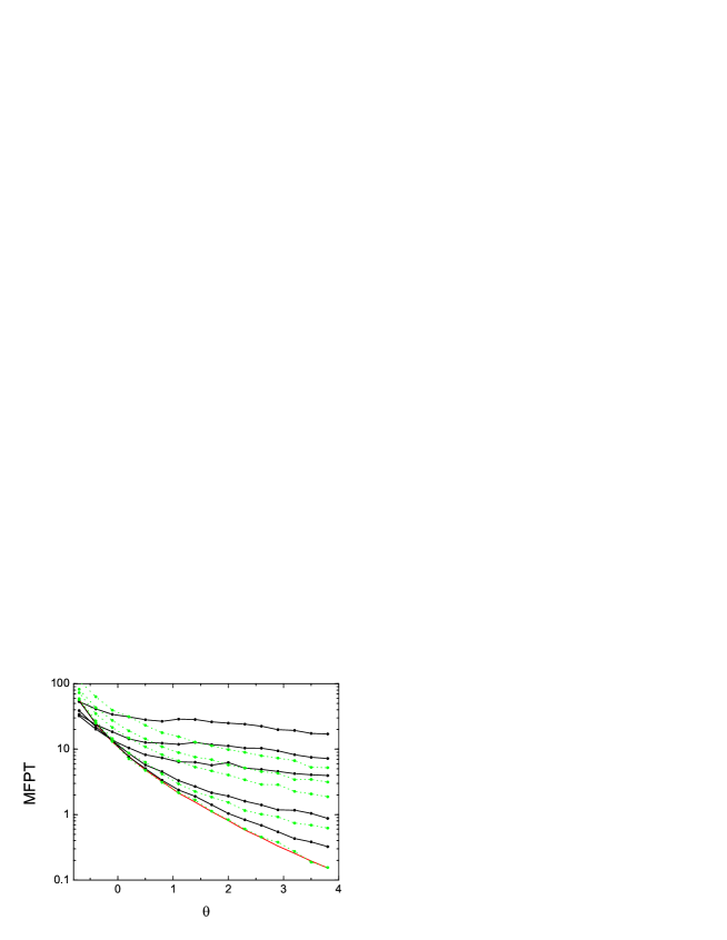
Figure 6: (Colour online) MFPT as a function of $\theta$ for finite $m$ and $\gamma$. The black solid lines correspond to the following values of $m$ (from bottom to top): 0.001, 0.01, 0.1, 1, 10 and $\gamma=100$. Dependence on $\gamma$ for $m=0$ is marked by green dotted lines: $\gamma=1000$, 10, 1, 0.5, 0.2 (from bottom to top). Other parameters: $\alpha=1.5$, $\beta=1$, $A=1$ and $B=0.1$. Result for the Stratonovich interpretation is marked by the red solid line without symbols.

IV Summary and conclusions

We have studied a one-dimensional dynamics of a massive particle subjected to the general Lévy stable noise, both additive and multiplicative. The driving noise has been represented by the generalised Ornstein-Uhlenbeck process and then the finite noise relaxation time has been taken into account. In the linear case, the dynamical variable $x$ is governed by the Lévy distribution and the parameter $\alpha$ is the same as for the driving noise. Therefore, diffusion is always accelerated. Distribution converges with time to the white-noise and massless case. Fractional moments rise with time; the rate decreases with the stability index $\alpha$ and the damping coefficient $\beta$. Inertia and noise relaxation time influence the rate of convergence to the asymptotic distribution.

The $x$-dependence of the multiplicative noise modifies the distribution. Slopes of the tail depend on the multiplicative factor $G(x)$, which was assumed in the algebraic form, and variance is finite if $G(x)$ falls sufficiently fast. Variance rises sub-linearly with time for $t\gg 1$ which indicates the subdiffusion. Those conclusions are valid for any noise relaxation parameter $\gamma$. The limit $\gamma\to\infty$ is of particular importance; the distribution in this limit coincides with Eq.(26). Therefore, the limit of the Langevin equation driven by the generalised Ornstein-Uhlenbeck process produces the same result as the formal variable change in the Langevin equation for the white-noise case. The influence of inertia is more subtle. It favours an expansion of the distribution if $m$ is small but for large $m$ distribution shrinks to the delta function. However, even in the limit $m\to\infty$ a little tail remains and it makes the variance divergent. In the white-noise limit, that tail agrees with the distribution in the Itô interpretation. On the other hand, the Stratonovich interpretation is valid for the small mass. Those conclusions are similar to the case of the normal distribution kup . Since slowly falling tails have been encountered only for the extremely large masses, convergent variance is by no means exceptional for the Lévy stable processes: it emerges if intensity of the multiplicative noise diminishes sufficiently fast. The finite noise relaxation time and inertia affect the barrier penetration: the calculated MFPT rises with both the memory parameter $1/\gamma$ and the particle mass. In the white-noise limit MFPT converges to the Stratonovich result.

The above analysis demonstrates that the Langevin formalism with the multiplicative Lévy noise predicts heavy, algebraic tails of the probability density distribution and the index $\mu$ can assume arbitrarily large values. As a consequence, moments of an arbitrarily high order may be convergent. $\mu$ depends not only on $\alpha$ and $\theta$, as it is the case for the massless particle, but also on the inertia. Those conclusions suggest that the presented formalism may be well suited to describe processes characterised by a variety of the algebraic slopes of the distribution sta ; gab ; sche . In the field of finance, a traditional Black-Scholes model of option pricing, which includes the additive Gaussian noise, can be generalised by introducing the Lévy flights. Need of such a generalisation is obvious cart but, since variance of the additive Lévy process is infinite, a truncation of the distribution becomes necessary. On the other hand, the first-order equation, like the Black-Scholes equation, with the multiplicative noise predicts sufficiently steep distribution slopes to ensure the finite variance also without any truncation if the stochastic integral is understood in the Stratonovich sense. The present paper justifies this interpretation for the first-order stochastic equations: it demonstrates that distribution slopes are robust in respect to the noise relaxation time – which is always finite for realistic problems – and the white-noise limit exists.

References

- (1) H. E. Stanley, Physica A 318, 279 (2003).
- (2) X. Gabaix, P. Gopikrishnan, V. Plerou, and H. E. Stanley, Nature 423, 267 (2003).
- (3) D. Schertzer, M. Larchevêque, J. Duan, V. V. Yanovsky, and S. Lovejoy, J. Math. Phys. 42, 200 (2001).
- (4) A. Chechkin, V. Gonchar, J. Klafter, R. Metzler, and L. Tanatarov, Chem. Phys. 284, 233 (2002).
- (5) R. Metzler and J. Klafter, Phys. Rep. 339, 1 (2000).
- (6) T. Srokowski, Physica A 390, 3077 (2011).
- (7) M. E. J. Newman, Contemp. Phys. 46, 323 (2005).
- (8) M. Park, N. Kleinfelter, and J. H. Cushman, Phys. Rev. E 72, 056305 (2005).
- (9) B. O’Shaughnessy and I. Procaccia, Phys. Rev. Lett. 54, 455 (1985).
- (10) R. Metzler and T. F. Nonnenmacher, J. Phys. A 30, 1089 (1997).
- (11) D. Brockmann and T. Geisel, Phys. Rev. Lett. 90, 170601 (2003).
- (12) A. Manor and N. M. Shnerb, Phys. Rev. Lett. 103, 030601 (2009).
- (13) A. La Cognata, D. Valenti, A. A. Dubkov, and B. Spagnolo, Phys. Rev. E 82, 011121 (2010).
- (14) T. Srokowski, Phys. Rev. E 80, 051113 (2009).
- (15) P. Hänggi and P. Jung, in Advances in Chemical Physics, edited by I. Prigogine and S. A. Rice, vol. 89 (John Wiley & Sons, Inc., Hoboken, NJ, USA, 2007).
- (16) J. N. Teramae, H. Nakao, and G. B. Ermentrout, Phys. Rev. Lett. 102, 194102 (2009).
- (17) R. Short, L. Mandel, and R. Roy, Phys. Rev. Lett. 49, 647 (1982).
- (18) R. Kubo, Fluctuation, Relaxation and Resonance in Magnetic Systems (Oliver and Boyd, London, 1982).
- (19) S. E. Mangioni, R. R. Deza, R. Toral, and H. S. Wio, Phys. Rev. E 61, 223 (2000).
- (20) E. Wong and M. Zakai, Ann. Math. Stat. 36, 1560 (1965).
- (21) R. Kupferman, G. A. Pavliotis, and A. M. Stuart, Phys. Rev. E 70, 036120 (2004).
- (22) J. M. Sancho and A. Sanchez, Eur. Phys. J. B 16, 127 (2000).
- (23) B. J. West and V. Seshardi, Physica A 113, 203 (1982).
- (24) S. Jespersen, R. Metzler, and H. C. Fogedby, Phys. Rev. E59, 2736 (1999).
- (25) P. Garbaczewski and R. Olkiewicz, J. Math. Phys. 41, 6843 (2000).
- (26) V. V. Yanovsky, A. V. Chechkin, D. Schertzer, and A. V. Tur, Physica A 282, 13 (2000).
- (27) E. Barkai, Phys. Rev. E68, 055104 (2003).
- (28) P. Embrechts and M. Maejima, Selfsimilar Processes (Princeton University Press, Princeton, 2002).
- (29) I. Eliazar and J. Klafter, Physica A 376, 1 (2007).
- (30) T. Srokowski, Acta Phys. Polon. B 42, 3 (2011).
- (31) R. N. Mantegna and H. E. Stanley, Phys. Rev. Lett. 73, 2946 (1994).
- (32) J. L. Doob, Ann. Math. 43, 351 (1942).
- (33) A. M. Mathai and R. K. Saxena, The -function with Applications in Statistics and Other Disciplines (Wiley Eastern Ltd., New Delhi, 1978).
- (34) H. M. Srivastava, K. C. Gupta, and S. P. Goyal, The -functions of one and two variables with applications (South Asian Publishers, New Delhi, 1982).
- (35) A. Schenzle and H. Brand, Phys. Rev. A 20, 1628 (1979).
- (36) N. G. van Kampen, J. Stat. Phys. 24, 175 (1981).
- (37) R. Graham and A. Schenzle, Phys. Rev. A 25, 1731 (1982).
- (38) O. Carrillo, M. Ibañes, J. García-Ojalvo, J. Casademunt, and J. M. Sancho, Phys. Rev. E 67, 046110 (2003).
- (39) C. W. Gardiner, Handbook of Stochastic Methods for Physics, Chemistry and the Natural Sciences (Springer-Verlag, Berlin, 1985).
- (40) G. Volpe, L. Helden, T. Brettschneider, J. Wehr, and C. Bechinger, Phys. Rev. Lett. 104, 170602 (2010).
- (41) T. Srokowski, Physica A 388, 1057 (2009).
- (42) T. Srokowski, Phys. Rev. E 81, 051110 (2010).
- (43) In contrast to the case , the shape of the density distribution for does not depend on the specific interpretation of the stochastic integral. For the Itô case, the exact solution of the corresponding Fokker-Planck equation predicts a stretched-Gaussian shape, , for large (H. G. E. Hentschel and I. Procaccia, Phys. Rev. A 29, 1461 (1984)). The same form follows when we apply the transformation (25) to the Gaussian.
- (44) A. Björk and G. Dahlquist, Numeriska Metoder (Liber Grafiska AB, Stockholm, 1969).
- (45) A. Ralston, A First Course in Numerical Analysis (McGraw-Hill, New York, 1965).
- (46) A. Janicki and A. Weron, Simulation and Chaotic Behavior of -Stable Stochastic Processes (Marcel Dekker, New York, 1994).
- (47) P. Hänggi, P. Talkner, and M. Borkovec, Rev. Mod. Phys. 62, 251 (1990).
- (48) P. D. Ditlevsen, Phys. Rev. E 60, 172 (1999).
- (49) B. Dybiec, E. Gudowska-Nowak, and P. Hänggi, Phys. Rev. E 75, 021109 (2007).
- (50) A. Cartea and D. del-Castillo-Negrete, Physica A 374, 749 (2007).