Classical Orbital Magnetic Moment in a Dissipative Stochastic System

Abstract

We present an analytical treatment of the dissipative-stochastic dynamics of a charged classical particle confined bi-harmonically in a plane with a uniform static magnetic field directed perpendicular to the plane. The stochastic dynamics gives a steady state in the long-time limit. We have examined the orbital magnetic effect of introducing a parametrized deviation $(\eta-1)$ from the second fluctuation-dissipation (II-FD) relation that connects the driving noise and the frictional memory kernel in the standard Langevin dynamics. The main result obtained here is that the moving charged particle generates a finite orbital magnetic moment in the steady state, and that the moment shows a crossover from para- to dia-magnetic sign as the parameter $\eta$ is varied. It is zero for $\eta=1$ that makes the steady state correspond to equilibrium, as it should. The magnitude of the orbital magnetic moment turns out to be a non-monotonic function of the applied magnetic field, tending to zero in the limit of an infinitely large as well as an infinitesimally small magnetic field. These results are discussed in the context of the classic Bohr-van Leeuwen theorem on the absence of classical orbital diamagnetism. Possible realization is also briefly discussed.

PACS numbers:

05.40.-a, 05.10.Gg, 75.20.-g.

The Bohr-van Leeuwen (BvL) theorem [1]–[3] on the stated absence of orbital diamagnetism for a classical system of charged particles in equilibrium has been one of the surprises of physics [4]. The static external magnetic field exerts a Lorentz force on the moving charged particle, acting at right angle to its instantaneous velocity (${\bf v}$). While such a gyroscopic force does no work on the particle, it does induce an orbital cyclotron motion that subtends an amperean current loop. The magnetic field associated with this current loop is expected to be non-zero, and directed oppositely to the externally applied magnetic field – the Lenz’ law. Hence the expectation of a finite orbital diamagnetic moment $q/2c(\bf{r}\times\bf{v})$ [5]. Yet, as is known well, the partition function for a classical system in equilibrium turns out to be independent of the applied magnetic field, thus giving a zero orbital magnetic moment. And this has been the surprise [4]. (The field independence of the classical partition function derives simply from the fact that the classical partition function involves integration of the canonical momentum over an infinite range for any given value of the conjugate coordinate, and thus the magnetic vector potential ($\bf{A}$) entering the Hamiltonian through minimal coupling $({\bf p}\rightarrow{\bf p}-\frac{q}{c}{\bf A})$ gets eliminated through a trivial shift of the momentum variable. This shift is, however, not allowed for a quantum system because of the canonical non-commutation involved there. Hence the stated quantum origin of the orbital magnetic moment in equilibrium – the Landau orbital diamagnetism [6]). A remarkably heuristic real-space explanation for the vanishing of the classical orbital moment was first suggested by Bohr [1] in terms of a cancellation of the orbital diamagnetic moment of the completed amperean orbits (Maxwell cycles) in the bulk interior by the paramagnetic moment subtended by the incompleted orbits skipping the bounding surface of the system in the opposite sense. This ‘edge current’ has a large arm-length, or leverage and, therefore, can effectively cancel out the bulk diamagnetic moment. The cancellation has indeed been demonstrated graphically for a simple planar geometry [7]. This real space-time picture is consistent with the zero orbital magnetic moment following from an exact analytical solution of the classical Langevin dynamics with a white noise describing the motion of the charged particle confined harmonically in two dimensions, with a uniform static magnetic field applied perpendicular to the plane [8]. Here, the steady state $(t\rightarrow\infty)$ orbital moment indeed vanishes for the given potential confinement (owing to the spring constant $k$ of the harmonic potential, providing a soft boundary). Interestingly, this null result persists in the limit $k\rightarrow 0$, provided it is taken after taking the limit $t\rightarrow\infty$. This suggests that in this case the stochastic particle dynamics has had time enough to sense (i.e., be influenced by) the confinement ($k$). On the other hand, the moment survives to a non-zero value if the order of the two limits is interchanged. (The effect of these so-called Darwinian limiting processes is also manifest in the case of the quantum version of the above Langevin treatment [9]). It is to be noted, however, that in the case of quantum Langevin equation the orbital moment tends to zero as the Planck constant is formally reduced to zero, i.e., in the classical limit, for which the noise term reduces to a classical white noise which is consistent with a local Stokes friction constant – in accord with the second fluctuation-dissipation (II-FD) theorem [10, 11]. This reasonably suggests to us that it may well be the constraint of the second fluctuation-dissipation relation that forces the orbital magnetic moment to vanish in the classical case. This is further supported by our recent numerical simulation [12]. Motivated by these observations, we have carried out an exact analytical calculation of the orbital magnetic moment of a charged particle confined bi-harmonically in two dimensions with a uniform static magnetic field applied normal to the xy-plane, but now with the proviso that the stochastic driving force (noise) is a sum of two uncorrelated noise terms – an exponentially correlated term and a delta-correlated term – and there is a parametrized $(\eta-1)$ deviation from the II-FD relation. Interestingly now, we do obtain a non-zero orbital magnetic moment in the infinite time limit – in the steady state. Moreover, the sign of the orbital magnetic moment turns out to show a dia- to para-magnetic crossover as the parameter $\eta$ is tuned through $\eta=1$, where the moment vanishes. In the following we present an exact analytical treatment of this dissipative-stochastic system and discuss the results that follow.

Consider the classical dissipative-stochastic dynamics of a particle, of charge $-e$ and mass $m$, which is confined bi-harmonically in the $xy$-plane in the presence of a uniform static magnetic field $B$ applied perpendicular to the plane. The governing stochastic (Langevin) equations are

$$m\ddot{x}(t)=-kx(t)-\int_{0}^{t}\left(\frac{\Gamma}{t_{c}}e^{-(t-t^{\prime})/t_{c}}+\Gamma_{0}\delta(t-t^{\prime})\right)\dot{x}(t^{\prime}){\rm d}t^{\prime}-\frac{eB}{c}\dot{y}(t)+\xi_{x}(t)$$ (1a)

$$m\ddot{y}(t)=-ky(t)-\int_{0}^{t}\left(\frac{\Gamma}{t_{c}}e^{-(t-t^{\prime})/t_{c}}+\Gamma_{0}\delta(t-t^{\prime})\right)\dot{y}(t^{\prime}){\rm d}t^{\prime}+\frac{eB}{c}\dot{x}(t)+\xi_{y}(t),$$ (1b)

where $\xi_{i}(t)$ is the noise term with $\langle\xi_{i}(t)\rangle=0$, and

$$\langle\xi_{i}(t)\xi_{j}(t^{\prime})\rangle=\delta_{i,j}mk_{B}T\left(\frac{\gamma}{t_{c}}e^{-|t-t^{\prime}|/t_{c}}+2\eta\gamma_{0}\delta(t-t^{\prime})\right),$$ (2)

and we are interested in the long-time limit $t\rightarrow\infty$. Here $i=x,y$, and the angular brackets $\langle\cdots\rangle$ denote average over realizations of the two un-correlated noise terms – one a delta-correlated (white) noise and the other an exponentially correlated noise with a correlation time $t_{c}$. This sum of a white noise and an exponentially correlated noise, we believe, is the simplest non-Markovian gaussian process allowed by Doob’s theorem [13]. Further, $(\eta-1)$ parametrizes deviation from the II-FD relation as noted above.

It is convenient to introduce here the quantities $\Omega_{0}=\sqrt{k/m}$ (harmonic oscillator circular frequency), $\frac{eB}{mc}=\Omega_{c}$ (cyclotron circular frequency), and $\frac{\Gamma}{m}=\gamma$ (the frictional relaxation frequency). We further define the following dimensionless parameters $\tau=\gamma t$ (dimensionless time), and $\omega_{0}=\frac{\Omega_{0}}{\gamma},\omega_{c}=\frac{\Omega_{c}}{\gamma}$ (dimensionless circular frequencies).

Following now the ’Landau trick’, the two coupled Langevin equations for the real displacements $x(\tau)$ and $y(\tau)$ as functions of the dimensionless time $\tau$, can be conveniently combined into a single Langevin equation for the complex displacement $z(\tau)\equiv x(\tau)+iy(\tau)$, giving:

$$\ddot{z}(\tau)=-\omega_{0}^{2}z(\tau)-\int_{0}^{\tau}\left(\frac{1}{\tau_{c}}e^{-(\tau-\tau^{\prime})/\tau_{c}}+\frac{\gamma_{0}}{\gamma}\delta(\tau-\tau^{\prime})\right)\dot{z}(\tau^{\prime}){\rm d}\tau^{\prime}+i\omega_{c}\dot{z}(\tau)+g(\tau)\\$$ (3)

with $\langle g(\tau)\rangle=0$ and $\langle g(\tau)g^{*}(\tau^{\prime})\rangle=\frac{2k_{B}T}{(m\gamma^{2})}\left(\frac{1}{\tau_{c}}e^{-(\tau-\tau^{\prime})/\tau_{c}}+(2\eta)\frac{\gamma_{0}}{\gamma}\delta(\tau-\tau^{\prime})\right)$.

Note the complex conjugation $(*)$ that we have introduced in $\langle g(\tau)g^{*}(\tau^{\prime})\rangle$ above, as the same will be needed in subsequent calculations. Also, we have changed over to the dimensionless time parameter $(\tau)$ , but have retained the same symbols for the dynamical variables without the risk of confusion. Inasmuch as the particle motion along the uniform magnetic field normal to the xy-plane decouples from that in the xy-plane, the present model equally well describes a 3-dimensional system. The orbital magnetic moment can now be re-written as

$$\langle M(\tau)\rangle=\frac{e\gamma}{2c}{\rm Im}\langle z(\tau)\dot{z}^{*}(\tau)\rangle.$$ (4)

It is convenient now to introduce the Laplace transform

$$\tilde{z}(s)=\int_{0}^{\infty}e^{-s\tau}z(\tau)d\tau,\ {\rm and}\ \tilde{\dot{z}}(s)=s\tilde{z}(s),$$ (5)

with the initial conditions $z(0)=0=\dot{z}(0)$ (without loss of generality, as we are interested in the steady state (long-time limit $\tau\rightarrow\infty)$. We obtain straightforwardly

$$\tilde{z}(s)=\frac{\tilde{g}(s)(1+\tau_{c}s)/\tau_{c}}{\left(s^{3}+\left(\frac{1}{\tau_{c}}+\frac{\gamma_{0}}{\gamma}-i\omega_{c}\right)s^{2}+\left(\omega_{0}^{2}+\frac{1}{\tau_{c}}+\frac{\gamma_{0}}{\gamma\tau_{c}}-\frac{i\omega_{c}}{\tau_{c}}\right)s+\frac{\omega_{0}^{2}}{\tau_{c}}\right)}$$ (6)

and

$$\tilde{\dot{z}}(s)=\frac{s(1+\tau_{c}s)\tilde{g}(s)/\tau_{c}}{\left(s^{3}+\left(\frac{1}{\tau_{c}}+\frac{\gamma_{0}}{\gamma}-i\omega_{c}\right)s^{2}+\left(\omega_{0}^{2}+\frac{1}{\tau_{c}}+\frac{\gamma_{0}}{\gamma\tau_{c}}-\frac{i\omega_{c}}{\tau_{c}}\right)s+\frac{\omega_{0}^{2}}{\tau_{c}}\right)},$$ (7)

where we have used $\tilde{\dot{z}}(s)=s\tilde{z}(s)$, with the initial conditions $z(0)=\dot{z}(0)=0$ as noted above. In order to inverse-Laplace transform the expressions above, it is convenient to introduce the factorized denominator

$$D(s) =\left(s^{3}+\left(\frac{1}{\tau_{c}}+\frac{\gamma_{0}}{\gamma}-i\omega_{c}\right)s^{2}+\left(\omega_{0}^{2}+\frac{1}{\tau_{c}}+\frac{\gamma_{0}}{\gamma\tau_{c}}-\frac{i\omega_{c}}{\tau_{c}}\right)s+\frac{\omega_{0}^{2}}{\tau_{c}}\right)$$ (8)

$$\equiv(s-s_{1})(s-s_{2})(s-s_{3}),$$

where $s_{i}(i=1,2,3)$ are the three roots of the cubic denominator $D(s)$. These roots are readily obtained following the Cardano procedure. We can then write $\tilde{z}(s)$ and $\tilde{\dot{z}}(s)$ as partial fractions

$$\tilde{z}(s)=\sum_{i}\frac{a_{i}}{s-s_{i}}\tilde{g}_{z}(s),$$ (9)

and

$$\tilde{\dot{z}}(s)=\sum_{i}\frac{A_{i}}{s-s_{i}}\tilde{g}_{z}(s),$$ (10)

where $\{a_{i}\}$ are given as solutions of the set of equations

$$a_{1}+a_{2}+a_{3}=0$$

$$a_{1}(s_{2}+s_{3})+a_{2}(s_{3}+s_{1})+a_{3}(s_{1}+s_{2})=-1$$

$$a_{1}s_{2}s_{3}+a_{2}s_{3}s_{1}+a_{3}s_{1}s_{2}=\frac{1}{\tau_{c}},$$ (11)

and similarly, $\{A_{i}\}$ are given by

$$A_{1}+A_{2}+A_{3}=1$$

$$A_{1}(s_{2}+s_{3})+A_{2}(s_{3}+s_{1})+A_{3}(s_{1}+s_{2})=-\frac{1}{\tau_{c}}$$

$$A_{1}s_{2}s_{3}+A_{2}s_{3}s_{1}+A_{3}s_{1}s_{2}=0,$$ (12)

In terms of the above, we now have the inverse Laplace transforms as

$$z(\tau)=\sum_{i}a_{i}\int_{0}^{\tau}e^{s_{i}(\tau-\tau^{\prime})/\tau_{c}}g(\tau^{\prime})d\tau^{\prime}$$ (13a)

and

$$\dot{z}(\tau)=\sum_{j}A_{j}\int_{0}^{\tau}e^{s_{j}(\tau-\tau^{\prime\prime})/\tau_{c}}g(\tau^{\prime\prime})d\tau^{\prime\prime}.$$ (13b)

With this, the orbital magnetic moment in Eq. (4) turns out to be

$$\langle M(\tau)\rangle =\left(\frac{e}{mc}\right)\left(\frac{k_{B}T}{\gamma\tau_{c}^{3}}\right){\rm Im}\sum_{i,j=1,2,3}a_{i}A_{j}^{*}\int\!\!\!\!\!\int\limits_{0}^{\tau}\left[e^{s_{i}(\tau-\tau^{\prime})/\tau_{c}}e^{s_{j}^{*}(\tau-\tau^{\prime\prime})/\tau_{c}}e^{-|\tau^{\prime}-\tau^{\prime\prime}|/\tau_{c}}\right.$$ (14)

$$\left.+2\eta\frac{\gamma_{0}\tau_{c}}{\gamma}e^{s_{i}(\tau-\tau^{\prime})/\tau_{c}}e^{s_{j}^{*}(\tau-\tau^{\prime\prime})/\tau_{c}}\delta(\tau^{\prime}-\tau^{\prime\prime})\right]d\tau^{\prime}d\tau^{\prime\prime},$$

where Im denotes the imaginary part. Straightforward integration gives the $\tau\rightarrow\infty$ (steady-state) limit for the orbital magnetic moment as

$$M(\infty) =\left(\frac{e}{mc}\right)\left(\frac{k_{B}T}{\gamma\tau_{c}^{3}}\right){\rm Im}\sum_{i,j=1,2,3}a_{i}A_{j}^{*}\left[\left(\frac{1}{\frac{1}{\tau_{c}}+s_{j}^{*}}\right)\right.$$ (15)

$$\left.\times\left\{\frac{2}{\tau_{c}(s^{*}_{j}-\frac{1}{\tau_{c}})(s_{i}+s_{j}^{*})}+\frac{1}{(s_{i}-\frac{1}{\tau_{c}})}\right\}-2\eta\frac{\gamma_{0}}{\gamma}\tau_{c}\left(\frac{1}{s_{i}+s_{j}^{*}}\right)\right].$$

After some simplification, the above expression for the orbital magnetic moment $M(\infty)$ reduces to

$$\mu\equiv\frac{M(\infty)}{(\frac{ek_{B}T}{mc\gamma\tau_{c}})}=-2(\eta-1)\frac{\gamma_{0}\tau_{c}}{\gamma}{\rm Im}\sum_{i,j=1,2,3}a_{i}A_{j}^{*}\left(\frac{1}{s_{i}+s_{j}^{*}}\right)$$ (16)

In Fig. 1, we have plotted the limiting steady-state value of the dimensionless orbital magnetic moment $\mu$ against the dimensionless applied magnetic field $\beta(=\frac{eB}{mc\gamma})$, where $\eta$ parametrizes the II-FD violation and is varied over the range 0.5–2.0. As we are interested here mainly in the matter of principles, we have made a simple choice for the dimensionless parameters involved, namely $\frac{1}{\tau_{c}}=\omega_{0}=1$ and $\frac{\gamma_{0}}{\gamma}=0.5$ (the strength of the white noise relative to the exponentially correlated noise).

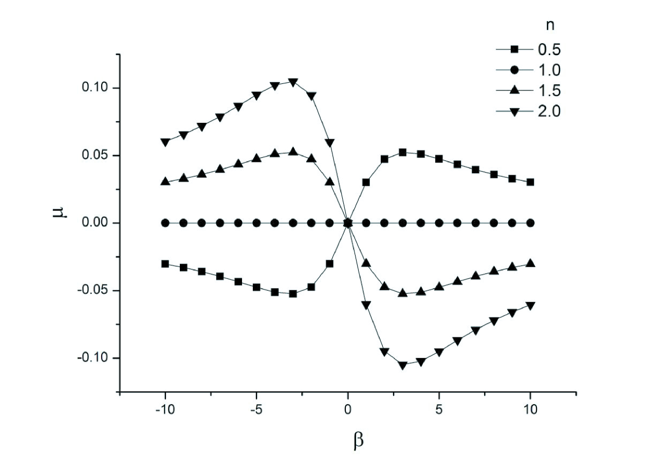
Figure 1: Plot of dimensionless magnetic moment $\mu$ against dimensionless magnetic field $\beta$ for four different values of $\eta$ that parametrizes deviation from the II-FD relation. It clearly shows a dia- to para-magnetic crossover as $\eta$ is varied through $\eta=1$. Also, the moment tends to zero in the limit of zero as well as large magnetic field $\beta$.

As we observe the field-induced orbital magnetic moment is clearly non-zero in the steady state. There is a crossover from the paramagnetic to the diamagnetic sign as the parameter $\eta$ is tuned from $\eta=0.5$ to $\eta=2.0$. This crossover is a surprise. The magnetic moment is zero for $\eta=1$, which corresponds to the canonical II-FD consistent (equilibrium) state. Hence no violation of the BvL theorem. The orbital magnetic moment is obviously zero for zero magnetic field; but, not so obviously it tends to zero for large magnetic field as well. The latter behaviour can, however, be understood from the following, namely that the radius/frequency of the cyclotron orbit tends to zero/infinity as the applied magnetic field is made infinitely large [4]. The fact that the orbital magnetic moment can be paramagnetic in certain range of the II-FD deviation parameter $\eta$ is significant in that, unlike diamagnetism, it leads to a positive feedback for a collection of charged particles in such a classical system – it can give an enhancement of the orbital paramagnetism.

Physical realization of such a classical system in the laboratory is admittedly somewhat demanding. One needs to create a dilute (highly non-degenerate) gas of charged particles (e.g., electrons/holes) at sufficiently high temperatures, and confined on a mesoscopic scale in the presence of a static magnetic field. The temperature has to be high enough so as to wash out the quantum effects, namely the discreteness of the quantized level spacings owing to the mesoscopic confinement. Now, the II-FD violating parameter $(\eta-1)$ necessarily requires a non-equilibrium steady-state condition. This is the real problem for an experimental realization. One is tempted to think that such a non-equilibrium steady state may be induced through a noisy laser excitation, e.g., the Kubo-Anderson non-Markovian noise [14, 15], of charged particles confined in an optical tweezer [16]. There is, however, a problem here involving the energy injected by the laser, its dissipation in the system and the associated rise of temperature. In fact, one necessarily needs to have a two-temperature configuration. Thus, e.g., a possible physical realization of our model can, in principle, have charged particles in contact with a thermal reservoir at one temperature, while another type of neutral particles is in contact with the reservoir at a different temperature. Then particle collisions will ensure a stationary (steady-state) non-equlibrium state with flow of energy between the reservoirs. This then according to our model calculattion should give a non-zero orbital magnetic moment in an externally applied magnetic field [17].

Given that classically a static magnetic field does no work on a moving charged particle, our model calculation giving a non-equilibrium steady-state solution in the presence of a static magnetic field could lead to some insightful molecular dynamical (MD) simulations when appropriately thermostatted [18]. Also, it has a significant bearing on the work related to generalized fluctuation-dissipation theorem for steady-state systems [19].

In conclusion, we have presented an exact analytical treatment of a classical dissipative-stochastic model system in a uniform static magnetic field, which is found to give a finite orbital magnetic moment in the steady state. Interestingly, we find that there is a crossover from the diamagnetic to the paramagnetic sign of the magnetic moment as function of a parametrized deviation from the second fluctuation-dissipation relation. We think that these results do complement, rather than violate the classic Bohr-van Leeuwen theorem.

The author would like to thank A.A. Deshpande and K. V. Kumar for many discussions. The author would also like to thank the referee for constructive criticisms.

References

- [1] J.H.V. Leeuwen, Journal de Physique 2, 361 (1921).
- [2] N. Bohr, Studies over Metallerners Elektrontheori, Ph.D. thesis, Copenhagen, 1911.
- [3] J.H.V. Vleck, The Theory of Electric and Magnetic Susceptibilities (Oxford University Press, London, 1932).
- [4] R.E. Peierls, Surprises in Theoretical Physics (Princeton University Press, Princeton, 1979). The fact that diamagnetism was known much earlier, indeed from the time of Faraday, its absence for a classical system could be viewed as the first macroscopic evidence for the incompleteness of classical (statistical) mechanics.
- [5] J.D. Jackson, Classical Electrodynamics (John Wiley, New York, 1975).
- [6] L.D. Landau, Zeits. f. Physik 64, 629 (1930).
- [7] S.K. Ma, Statistical Mechanics (World Scientific, Singapore, 1985) p. 283.
- [8] N. Kumar and A.M. Jayannavar, J. Phys. A 14, 1399 (1981).
- [9] S. Dattagupta and J. Singh, Phys. Rev. Lett. 79, 961 (1997); S. Dattagupta, N. Kumar and A.M. Jayannavar, Curr. Sci. 8, 863 (2001).
- [10] R. Kubo, Rep. Prog. Phys. 29, 255 (1966).
- [11] V. Balakrishnan, Pramana 12, 301 (1979).
- [12] A. A. Deshpande, K. V. Kumar and N. Kumar (unpublished).
- [13] J.L. Doob, Selected Papers on Noise and Stochastic Processes, ed. N. Wax (Dover, New York, 1954) p. 319.
- [14] R. Kubo, J. Phys. Soc. Jpn 9, 935 (1954).
- [15] P.W. Anderson, J. Phys. Soc. Jpn. 9, 316 (1954).
- [16] T. Li et al., Science 328, 1673 (2010); R. Huang et al., Nature Physics, p.1, 27 March 2011.
- [17] The author would like to thank the referee for suggesting the possible physical realization of our model.
- [18] W.G. Hoover, Phys. Rev. A 31, 1695 (1985); S. Nos , J. Chem. Phys. 81, 511 (1984).
- [19] J. Prost, J.-F. Joanny and J.M.R. Parrondo, Phys. Rev. Lett. 103, 090601 (2009)