Photon-photon production of lepton, quark and meson pairs in peripheral heavy ion collisions

Abstract

We review our recent results on exclusive production of $\mu^{+}\mu^{-}$, heavy quark-antiquark, and meson-antimeson pairs in ultraperipheral, ultrarelativistic heavy ion collisions.

1 Introduction

Ultrarelativistic collisions of heavy ions provide a nice oportunity to study photon-photon collisions [1]. One can expect an enhancement of the cross section for the reactions of this type compared to proton-proton or $e^{+}e^{-}$ collisions which is caused by a large charges of the colliding ions. In this type of reactions virtual (almost real) photons couple to the nucleus as a whole. Naively the enhancement of the cross section is proportional to $Z_{1}^{2}Z_{2}^{2}$ which is a huge factor. We have discussed recently that the inclusion of realistic charge distributions and realistic nucleus charge form factor makes the cross section smaller than the naive predictions. Many processes has been discussed in the literature. Recently we have also studied some of them.

We have discussed production of $\mu^{+}\mu^{-}$ pairs [2] heavy-quark heavy-antiquark pairs [3] as well as production of two mesons: $\rho^{0}\rho^{0}$ pairs [4], $\pi^{+}\pi^{-}$ pairs [5] as well as of $D\bar{D}$ meson pairs [6].

Here we shall summarize the recent works.

2 Formalism

2.1 Equivalent Photon Approximation

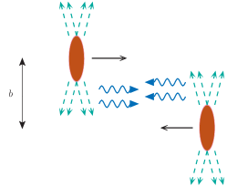
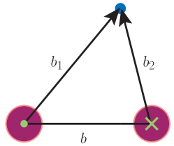
Figure 1: A schematic picture of the collision and the quantities used in the impact parameter calculation.

The equivalent photon approximation is a standard semi–classical alternative to the Feynman rules for calculating cross sections of electromagnetic interactions [7]. This picture is illustrated in Fig. 1 where one can see a fast moving nucleus with the charge $Ze$. Due to the coherent action of all protons in the nucleus, the electromagnetic field surrounding (the dashed lines are lines of electric force for a particles in motion) the ions is very strong. This field can be viewed as a cloud of virtual photons. In the collision of two ions, these quasireal photons can collide with each other and with the other nucleus. The strong electromagnetic field is a source of photons that can induce electromagnetic reactions on the second ion. We consider very peripheral collisions i.e. we assume that the distance between nuclei is bigger than the sum of radii of the two nuclei. Fig. 1 explains also the quantities used in the impact parameter calculation. In the right panel we can see a view in the plane perpendicular to the direction of motion of the two ions. In order to calculate the cross section of a process it is convenient to introduce the following kinematic variables:

• $x=\omega/E_{A}$, where $\omega$ energy of the photon and the energy of the nucleus

• $E_{A}=\gamma Am_{proton}=\gamma M_{A}$ where $M_{A}$ is the mass of the nucleus and $E_{A}$ is the energy of the nucleus

Below we consider a generic reaction $AA\to AAc_{1}c_{2}$ and later consider different examples when $c_{1}$ and $c_{2}$ are leptons, quarks or mesons. In the equivalent photon approximation the total cross section is calculated by the convolution:

$$\sigma\left(AA\rightarrow c_{1}c_{2}AA;s_{AA}\right)=\int{\hat{\sigma}}\left(\gamma\gamma\rightarrow c_{1}c_{2};W_{\gamma\gamma}=\sqrt{x_{1}x_{2}s_{AA}}\right){\rm d}n_{\gamma\gamma}\left(x_{1},x_{2},{\bf b}\right).$$ (1)

The luminosity function $dn_{\gamma\gamma}$ above can be expressed in term of flux factors of photons prescribed to each of the nucleus:

$${\rm d}n_{\gamma\gamma}\left(\omega_{1},\omega_{2},{\bf b}\right)=\int S^{2}_{abs}\left({\bf b}\right){\rm d^{2}}{\bf b}_{1}N\left(\omega_{1},{\bf b}_{1}\right){\rm d^{2}}{\bf b}_{2}N\left(\omega_{2},{\bf b}_{2}\right)\frac{{\rm d}\omega_{1}}{\omega_{1}}\frac{{\rm d}\omega_{2}}{\omega_{2}}.$$ (2)

The presence of the absorption factor $S^{2}_{abs}\left({\bf b}\right)$ assures that we consider only peripheral collisions, when the nuclei do not touch each other i.e. do not undergo nuclear breakup. In the first approximation this can be taken into account by the following approximation:

$$S^{2}_{abs}\left({\bf b}\right)=\theta\left({\bf b}-2R_{A}\right)=\theta\left(|{\bf b}_{1}-{\bf b}_{2}|-2R_{A}\right)\;.$$ (3)

In the present case, we concentrate on processes with final nuclei in the ground state. The electric field force can be expressed through the charge form factor of the nucleus [2].

The total cross section for the $AA\rightarrow c_{1}c_{2}AA$ process can be factorized into an equivalent photons spectra and the $\gamma\gamma\to c_{1}c_{2}$ subprocess cross section as:

$$\sigma\left(AA\rightarrow c_{1}c_{2}AA;s_{AA}\right)=\int{\hat{\sigma}}\left(\gamma\gamma\rightarrow c_{1}c_{2};\sqrt{4\omega_{1}\omega_{2}}\right)\,\theta\left(|{\bf b}_{1}-{\bf b}_{2}|-2R_{A}\right)$$

$$N\left(\omega_{1},{\bf b}_{1}\right)N\left(\omega_{2},{\bf b}_{2}\right){\rm d^{2}}{\bf b}_{1}{\rm d^{2}}{\bf b}_{2}\frac{{\rm d}\omega_{1}}{\omega_{1}}\frac{{\rm d}\omega_{2}}{\omega_{2}}\;.$$ (4)

We introduce the invariant mass of the $\gamma\gamma$ system: $W_{\gamma\gamma}=\sqrt{4\omega_{1}\omega_{2}}$. Additionally, we define $Y=\frac{1}{2}\left(y_{c_{1}}+y_{c_{2}}\right)$ rapidity of the outgoing $c_{1}c_{2}$ system. Making the following transformations:

$$\omega_{1}=\frac{W_{\gamma\gamma}}{2}e^{Y},\qquad\omega_{2}=\frac{W_{\gamma\gamma}}{2}e^{-Y}\;,$$ (5)

$$\frac{{\rm d}\omega_{1}}{\omega_{1}}\frac{{\rm d}\omega_{2}}{\omega_{2}}=\frac{2}{W_{\gamma\gamma}}{\rm d}W_{\gamma\gamma}{\rm d}Y\;,$$ (6)

$${\rm d}\omega_{1}{\rm d}\omega_{2}\to{\rm d}W_{\gamma\gamma}{\rm d}Y,\quad\left|\frac{\partial\left(\omega_{1},\omega_{2}\right)}{\partial\left(W_{\gamma\gamma},Y\right)}\right|=\frac{W_{\gamma\gamma}}{2}\;,$$ (7)

formula (4) can be written in an equivalent way as:

$$\sigma\left(AA\rightarrow c_{1}c_{2}AA;s_{AA}\right)=\int{\hat{\sigma}}\left(\gamma\gamma\rightarrow c_{1}c_{2};W_{\gamma\gamma}\right)\theta\left(|{\bf b}_{1}-{\bf b}_{2}|-2R_{A}\right)$$

$$N\left(\omega_{1},{\bf b}_{1}\right)N\left(\omega_{2},{\bf b}_{2}\right)\times{\rm d^{2}}{\bf b}_{1}{\rm d^{2}}{\bf b}_{2}\frac{W_{\gamma\gamma}}{2}{\rm d}W_{\gamma\gamma}{\rm d}Y\;.$$ (8)

Finally the cross section can be expressed as the five-fold integral:

$$\sigma\left(AA\rightarrow c_{1}c_{2}AA;s_{AA}\right)=\int{\hat{\sigma}}\left(\gamma\gamma\rightarrow\mu^{+}\mu^{-};W_{\gamma\gamma}\right)\theta\left(|{\bf b}_{1}-{\bf b}_{2}|-2R_{A}\right)$$

$$\times N\left(\omega_{1},{\bf b}_{1}\right)N\left(\omega_{2},{\bf b}_{2}\right)2\pi b_{m}\,{\rm d}b_{m}\,{\rm d}b_{x}\,{\rm d}b_{y}\frac{W_{\gamma\gamma}}{2}{\rm d}W_{\gamma\gamma}{\rm d}Y\,,$$ (9)

where $\vec{b}_{x}\equiv(b_{1x}+b_{2x})/2$, $\vec{b}_{y}\equiv(b_{1y}+b_{2y})/2$ and $\vec{b}_{m}=\vec{b}_{1}-\vec{b}_{2}$ have been introduced. The formula above is used to calculate the total cross section for the $AA\to AAc_{1}c_{2}$ reaction as well as distributions in $b=b_{m}$, $W_{\gamma\gamma}=M_{c_{1}c_{2}}$ and $Y(c_{1}c_{2})$.

Different forms of charge form factors of nucleus were used in the literature. We compare the equivalent photon spectra for realistic charge distribution and for the case of monopole form factor. A compact formula how the photon flux depends on the charge form factors can be found in [1].

$$N\left(\omega,b\right)=\frac{Z^{2}\alpha_{em}}{\pi^{2}}\frac{1}{b^{2}\omega}\left(\int u^{2}J_{1}\left(u\right)F\left(\sqrt{\frac{\left(\frac{b\omega}{\gamma}\right)^{2}+u^{2}}{b^{2}}}\right)\frac{1}{\left(\frac{b\omega}{\gamma}\right)^{2}+u^{2}}du\right)^{2},$$ (10)

where $J_{1}$ is the Bessel function of the first kind and $q$ is momentum of the quasireal photon. The calculations with the help of realistic form factor are rather laborious, so often a simpler formula with monopole form factor is used [8].

2.2 Charge form factor of nuclei

The charge distribution in nuclei is usually obtained from elastic scattering of electrons from nuclei [9]. The charge distribution obtained from those experiments is often parametrized with the help of two–parameter Fermi model [10]:

$$\rho\left(r\right)=\rho_{0}\left(1+\exp\left(\frac{r-c}{a}\right)\right)^{-1},$$ (11)

where $c$ is the radius of the nucleus, $a$ is the so-called diffiusness parameter of the charge density.

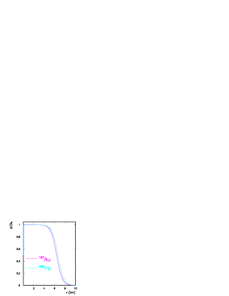
Figure 2: The ratio of $\rho$ the charge distibution to $\rho_{0}$, the density in the center of nucleus.

Fig. 2 shows the charge density normalized to unity. The correct normalization is: $\rho_{0,\,Au}(0)=\frac{0.1694}{A}fm^{-3}$ for Au and $\rho_{0,\,Pb}(0)=\frac{0.1604}{A}fm^{-3}$ for Pb.

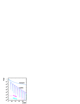
Figure 3: The moduli of the charge form factor $F_{em}\left(q\right)$ of the ${}^{197}Au$ and ${}^{208}Pb$ nuclei for realistic charge distributions. For comparison we show the monopole form factor for the same nuclei.

Mathematically the charge form factor is the Fourier transform of the charge distribution [9]:

$$F(q)=\int\frac{4\pi}{q}\rho\left(r\right)\sin\left(qr\right)rdr\;.$$ (12)

Fig. 3 shows the moduli of the form factor calculated from Eq.(12) as a function of momentum transfer. Here one can see many oscillations characteristic for relatively sharp edge of the nucleus. We show results for the gold (solid line) and lead (dashed line) nuclei for realistic charge distribution. For comparison we show the monopole form factor often used in the literature. The two form factors coincide only in a very limited range of $q$.

The monopole form factor [8]:

$$F(q^{2})=\frac{\Lambda^{2}}{\Lambda^{2}+q^{2}}.$$ (13)

leads to a simplification of many formulae for production of pairs of particles via photon-photon subprocess in nucleus-nucleus collisions. In our calculation $\Lambda$ is adjusted to reproduce root mean square radius $\Lambda=\sqrt{\frac{6}{<r^{2}>}}$ with the help of experimental data [10].

2.3 Exclusive production of $\mu^{+}\mu^{-}$ pairs

Elementary cross section for charged leptons can be calculated within Quantum Electrodynamics. Several groups have made relevant calculations (see e.g. [11, 12, 13, 14] and references therein).

Recently we have performed calculation of exclusive production of $\mu^{+}\mu^{-}$ and explored potential of RHIC and LHC in this respect. In Ref.[2] we have presented several distributions in muon rapidity and transverse momentum for RHIC and LHC experiments, including experimental acceptances. We have demonstrated how important is inclusion of realistic form factor in order to obtain realistic distributions of muons for RHIC and LHC. Many previous calculations in the literature concentrated rather on the total cross section and did not pay attention to differential distributions. Hovever, future experiments will measure the cross section in very limited part of the phase space. Here we wish to present only some selected examples.

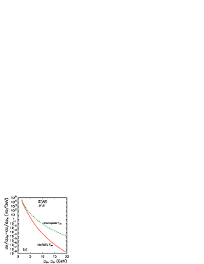
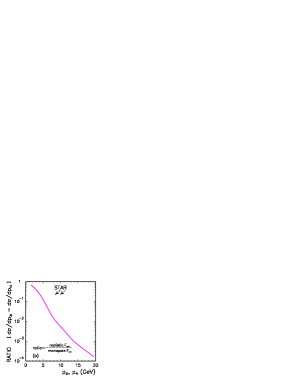
Figure 4: $\frac{{\rm d}\sigma}{{\rm d}p_{3t}}$ (left) and the ratio (right) for the STAR conditions: $y_{3},y_{4}\in(-1,1)$, $p_{3t},p_{4t}\geq$ 1 GeV and $W_{NN}=200$ GeV.

The distribution in the muon transverse momentum for STAR detector is shown in Fig.4. The STAR rapidity cuts -1 $<y_{3},y_{4}<$ 1 are taken here into account. As can be seen from the figure, the inclusion of realistic charge distribution is here extremely important. The relative effect of damping of the cross section with respect to the results with the monopole charge form factor (often used in the literature) is shown in the right panel. At $p_{t}$ = 10 GeV the damping factor is as big as 100! Experiments at RHIC have a potential to confirm this prediction.

The ALICE collaboration can measure only forward muons with psudorapidity 3 $<\eta<$ 4 and has relatively low cut on muon transverse momentum $p_{t}>$ 2 GeV. In Fig.5 (left panel) we show invariant mass distribution of dimuons for monopole and realistic form factors including the cuts of the ALICE apparatus. The bigger invariant mass, the bigger the difference between the two results. The same is true for distributions in muon transverse momenta (see the right panel).

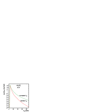
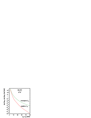
Figure 5: $\frac{{\rm d}\sigma}{{\rm d}W_{\gamma\gamma}}$ (left) and $\frac{{\rm d}\sigma}{{\rm d}p_{3t}}=\frac{{\rm d}\sigma}{{\rm d}p_{4t}}$ (right) for ALICE conditions: $y_{3},y_{4}=(3,4)$, $p_{3t},p_{4t}\geq$ 2 GeV.

2.4 Exclusive production of $c\bar{c}$ and $b\bar{b}$

In Fig.6,7,8,9 we show several photon-photon processes leading to the $Q\bar{Q}$ in the final state. In the following we shall discuss them one by one.

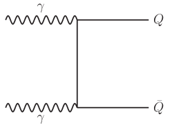
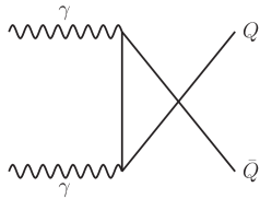
Figure 6: Representative diagrams for the Born amplitudes.

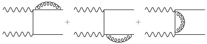
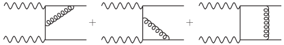
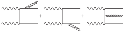
Figure 7: Representative diagrams for the leading–order QCD corrections.

=

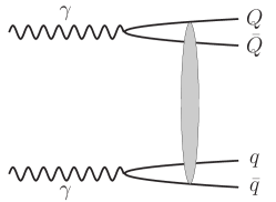
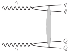
Figure 8: Representative diagrams for $Q\bar{Q}q\bar{q}$ production. The oval in the figure means a complicated interaction which is described here in the saturation model as explained in the main text.

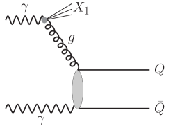
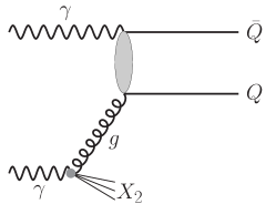
Figure 9: Representative diagrams for the single-resolved mechanism. The shaded oval means either t- or u- diagrams shown in Fig. 6.

Let us start with the Born direct contribution. The leading–order elementary cross section for $\gamma\gamma\to Q\bar{Q}$ as a function of $W_{\gamma\gamma}$ takes a simple form which differs from that for $\gamma\gamma\to l^{+}l^{-}$ by color factors and fractional charges of quarks.

In the current calculation we take the following heavy quark masses: $m_{c}=1.5$ GeV, $m_{b}=4.75$ GeV. It is obvious that the final $Q\bar{Q}$ state cannot be observed experimentally due to the quark confinement and rather heavy mesons have to be observed instead. Presence of additional few light mesons is rather natural. This forces one to include also more complicated final states.

In contrast to QED production of lepton pairs in photon-photon collisions, in the case of $Q\bar{Q}$ production one needs to include also higher-order QCD processes which are known to be rather significant. Here we include leading–order corrections only for the direct contribution. In $\alpha_{s}$-order there occur one-gluon bremsstrahlung diagrams ($\gamma\gamma\to Q\bar{Q}g$) and interferences of the Born diagram with self-energy diagrams (in $\gamma\gamma\to Q\bar{Q}$) and vertex-correction diagrams (in $\gamma\gamma\to Q\bar{Q}$). The relevant diagrams are shown in Fig.7. We have followed the approach presented in Ref. [15]. The QCD corrections can be written as:

$$\sigma_{\gamma\gamma\to Q\bar{Q}\left(g\right)}^{QCD}(W_{\gamma\gamma})=N_{c}e_{Q}^{4}\frac{2\pi\alpha_{em}^{2}}{W_{\gamma\gamma}^{2}}C_{F}\frac{\alpha_{s}}{\pi}f^{\left(1\right)}.$$ (14)

The function $f^{\left(1\right)}$ is calculated using a code provided by the authors of Ref. [15]. In the present analysis the scale of $\alpha_{s}$ is fixed at $\mu^{2}=4m_{Q}^{2}$.

We include also the subprocess $\gamma\gamma\to Q\bar{Q}q\bar{q}$, where $q$ ($\bar{q}$) are $u,\,d,\,s$, quarks (antiquarks). The cross section for this mechanism can be easily calculated in the color dipole framework [16, 17]. In the dipole–dipole approach [17] the total cross section for the $\gamma\gamma\to Q\bar{Q}$ production can be expressed as:

$$\sigma^{4q}_{\gamma\gamma\to Q\bar{Q}}\left(W_{\gamma\gamma}\right)$$

$$=\sum_{f_{2}\neq Q}\int\left|\Phi^{Q\bar{Q}}\left(\rho_{1},z_{1}\right)\right|^{2}\left|\Phi^{f_{2}\bar{f_{2}}}\left(\rho_{2},z_{2}\right)\right|^{2}\sigma_{dd}\left(\rho_{1},\rho_{2},x_{Qf}\right)d^{2}\rho_{1}dz_{1}d^{2}\rho_{2}dz_{2}$$

$$+\sum_{f_{1}\neq Q}\int\left|\Phi^{f_{1}\bar{f_{1}}}\left(\rho_{1},z_{1}\right)\right|^{2}\left|\Phi^{Q\bar{Q}}\left(\rho_{2},z_{2}\right)\right|^{2}\sigma_{dd}\left(\rho_{1},\rho_{2},x_{fQ}\right)d^{2}\rho_{1}dz_{1}d^{2}\rho_{2}dz_{2}\,,$$ (15)

where $\Phi^{Q\bar{Q}}\left(\rho,z\right)$ are the quark – antiquark wave functions of the photon in the mixed representation and $\sigma_{dd}$ is the dipole–dipole cross section. Eq.(15) is correct at sufficiently high energy $W_{\gamma\gamma}\gg 2m_{Q}$. At lower energies, the proximity of the kinematical threshold must be taken into account. In Ref. [16] a phenomenological saturation–model inspired parametrization for the azimuthal angle averaged dipole–dipole cross section has been proposed:

$$\sigma^{a,b}_{dd}=\sigma^{a,b}_{0}\left[1-\exp\left(-\frac{r^{2}_{\rm eff}}{4R^{2}_{0}\left(x_{ab}\right)}\right)\right].$$ (16)

Here, the saturation radius is defined as:

$$R_{0}\left(x_{ab}\right)=\frac{1}{Q_{0}}\left(\frac{x_{ab}}{x_{0}}\right)^{-\lambda/2}$$ (17)

and the parameter $x_{ab}$ which controls the energy dependence is given by:

$$x_{ab}=\frac{4m_{a}^{2}+4m_{b}^{2}}{W_{\gamma\gamma}^{2}}.$$ (18)

The effective radius is parametrized as $r_{\rm eff}^{2}=(\rho_{1}\rho_{2})^{2}/(\rho_{1}+\rho_{2})$ [16] . Some other parametrizations of the dipole-dipole cross section were also discussed in the literature. The cross section for the $\gamma\gamma\to Q\bar{Q}q\bar{q}$ process here is much bigger than the one corresponding to the tree-level Feynman diagram as it effectively resums higher-order QCD contributions.

As discussed in Ref. [17] the $Q\bar{Q}q\bar{q}$ component have very small overlap with the single-resolved component because of quite different final state, so adding them together does not lead to double counting. The cross section for the single-resolved contribution can be written as:

$$\sigma_{1-res}\left(s\right)=\int dx_{1}\left[g_{1}\left(x_{1},\mu^{2}\right)\hat{\sigma}_{g\gamma}\left(\hat{s}=x_{1}s\right)\right]+$$

$$\int dx_{2}\left[g_{2}\left(x_{2},\mu^{2}\right)\hat{\sigma}_{\gamma g}\left(\hat{s}=x_{2}s\right)\right],$$ (19)

where $g_{1}$ and $g_{2}$ are gluon distributions in photon $1$ or photon $2$ and $\hat{\sigma}_{q\gamma}$ and $\hat{\sigma}_{\gamma g}$ are elementary cross sections. In our calculation we take the gluon distribution from Ref. [18].

Elementary cross sections have been presented and discussed in Ref.[3]. Here we show only nuclear cross sections. In Fig. 10 we compare the contributions of the different mechanisms as a function of the photon–photon subsystem energy. For the Born case it is identical as a distribution in quark-antiquark invariant mass. In the other cases the photon–photon subsystem energy is clearly different than the $Q\bar{Q}$ invariant mass. These distributions reflect the energy dependence of the elementary cross sections. Please note a sizable contribution of the leading–order corrections close to the threshold and at large energies for the $c\bar{c}$ case. Since in this case $W_{\gamma\gamma}>M_{Q\bar{Q}}$, it becomes clear that the $Q\bar{Q}q\bar{q}$ contributions must have much steeper dependence on the $Q\bar{Q}$ invariant mass than the direct one which means that large $Q\bar{Q}$ invariant masses are produced mostly in the direct process. In contrast, small invariant masses (close to the threshold) are populated dominantly by the four–quark contribution. Therefore, measuring the invariant mass distribution one can disentangle some of the different mechanisms. As far as this is clear for the $c\bar{c}$ it is less transparent and more complicated for the $b\bar{b}$ production. In the last case the experimental decomposition may be in practice not possible.

Figure 10: The nuclear cross section as a function of photon–photon subsystem energy $W_{\gamma\gamma}$ in EPA. The solid line denotes the results corresponding to the Born amplitude ($c\bar{c}$ -left panel and $b\bar{b}$ -right panel). The leading–order QCD corrections are shown by the dash-dotted line. For comparison we show the differential distributions in the case when an additional pair of light quarks is produced in the final state (dashed lines) and for the single-resolved components (dotted line).

In Table 1 we show partial contribution of different subprocesses discussed above.

Table 1: Partial contributions of different mechanisms at $\sqrt{s_{NN}}$ = 5.5 TeV.

	$\sigma_{tot}$	Born	QCD-corr.	4-q	Sin.-res.
$c\overline{c}$	2.47 $mb$	42.5 %	14.6 %	27.1 %	15.8 %
$b\overline{b}$	10.83 $\mu b$	18.9 %	7.7 %	64.5 %	8.9 %

2.5 Exclusive production of $\pi^{+}\pi^{-}$ pairs

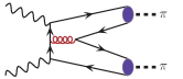
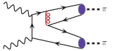
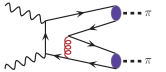
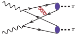
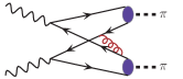
Figure 11: Typical Feynman diagrams describing the $\gamma\gamma\to(q\bar{q})(q\bar{q})\to\pi\pi$ amplitude in the LO pQCD.

In this subsection we discuss production of only “large” invariant mass $\pi^{+}\pi^{-}$ pairs. Brodsky and Lepage developed a formalism [19] how to calculate relevant cross section. Typical diagrams of the Brodsky-Lepage formalism are shown in Fig. 11. The invariant amplitude for the initial helicities of two photons can be written as the following convolution:

$$\mathcal{M}\left(\lambda_{1},\lambda_{2}\right)=\int_{0}^{1}dx\int_{0}^{1}dy\,\phi_{\pi}\left(x,\mu^{2}_{x}\right)T^{\lambda_{1}\lambda_{2}}_{H}\left(x,y,\mu^{2}\right)\phi_{\pi}\left(y,\mu^{2}_{y}\right),$$ (20)

where $\mu_{x}=\min\left(x,1-x\right)\sqrt{s(1-z^{2})}$, $\mu_{y}=\min\left(y,1-y\right)\sqrt{s(1-z^{2})}$; $z=\cos\theta$ [19]. We take the helicity dependent hard scattering amplitudes from Ref. [20]. These scattering amplitudes are different for $\pi^{+}\pi^{-}$ and $\pi^{0}\pi^{0}$. The distribution amplitudes are subjected to the ERBL pQCD evolution [21, 22]. The scale dependent quark distribution amplitude of the pion can be expanded in term of the Gegenbauer polynomials:

$$\phi_{\pi}\left(x,\mu^{2}\right)=\frac{f_{\pi}}{2\sqrt{3}}6x\left(1-x\right)\sum_{n=0}^{\infty^{\prime}}C_{n}^{3/2}\left(2x-1\right)a_{n}\left(\mu^{2}\right)\;.$$ (21)

where $f_{\pi}$ is the pion decay constant.

Different distribution amplitudes have been used in the past. Recently Wu and Huang [23] proposed a new distribution amplitude (based on a light-cone wave function):

$$\phi_{\pi}\left(x,\mu_{0}^{2}\right)=\frac{\sqrt{3}A\,m_{q}\beta}{2\sqrt{2}\pi^{3/2}f_{\pi}}\sqrt{x\left(1-x\right)}\left(1+B\times C_{2}^{3/2}\left(2x-1\right)\right)$$

$$\left(\mbox{Erf}\left[\sqrt{\frac{m_{q}^{2}+\mu_{0}^{2}}{8\beta^{2}x\left(1-x\right)}}\right]-\mbox{Erf}\left[\sqrt{\frac{m_{q}^{2}}{8\beta^{2}x\left(1-x\right)}}\right]\right).$$

(22)

The pion distribution amplitude at the initial scale is controlled by the parameter B. They have found that the BABAR data for pion transition form factor at low and high transferred four-momentum squared regions can be described by setting $B\approx$ 0.6. This pion distribution amplitude is rather similar to the well know Chernyak-Zhitnitsky [24] distribution amplitude ($\phi_{\pi\,CZ}=30x(1-x)(2x-1)^{2}$). In the following we shall use $B=$ 0.6 and $m_{q}=$ 0.3 GeV. Then $A=$ 16.62 GeV^-1 and $\beta=$ 0.745 GeV.

The total (angle integrated) cross section for the process can be expressed in terms of the amplitude of the process discussed above as:

$$\sigma_{\gamma\gamma\to\pi\pi}=\int\frac{2\pi}{4\cdot 64\pi^{2}W^{2}}\frac{p}{q}\sum_{\lambda_{1},\lambda_{2}}\left|\mathcal{M}\left(\lambda_{1},\lambda_{2}\right)\right|^{2}dz\;,$$ (23)

where the factor $4$ is due to averaging over initial photon helicities.

The hand-bag model was proposed as an alternative for the leading term Brodsky-Lepage pQCD approach [25]. It is based on the philosophy that the present energies are not sufficient for the dominance of the leading pQCD terms. As in the case of BL pQCD the hand-bag approach applies at large Mandelstam variables $s\sim-t\sim-u$ i.e. at large momentum transfers. Diehl, Kroll and Vogt presented a sketchy derivation [25] obtaining that the angular dependence of the amplitude is $\propto 1/\sin^{2}\theta$. In this approach the ratio of the cross section for the $\pi^{0}\pi^{0}$ process to that for the $\pi^{+}\pi^{-}$ process does not depend on $\theta$ and is $\frac{1}{2}$. The nonperturbative object $R_{\pi\pi}\left(s\right)$ in the hand-bag amplitude, describing transition from a quark pair to a meson pair, cannot be calulated from first principles. In Ref. [25] the form factor was parametrized in terms of the valence and non-valence form factors as:

$$R_{\pi\pi}\left(s\right)=\frac{5}{9s}a_{u}\left(\frac{s_{0}}{s}\right)^{n_{u}}+\frac{1}{9s}a_{s}\left(\frac{s_{0}}{s}\right)^{n_{s}}.$$ (24)

The $a_{u}$, $n_{u}$, $a_{s}$ and $n_{s}$ values found from the fit in Ref. [25] slightly depend on energy. For simplicity we have averaged these values and used: $a_{u}=$ 1.375 GeV², $n_{u}=$ 0.4175, $a_{s}=$ 0.5025 GeV² and $n_{s}=$ 1.195.

In Ref.[5] we have discussed in detail elementary cross sections as a function of photon-photon energy and as a function of $\cos(\theta)$. Here we will present only nuclear cross sections calculated within EPA discussed in the theoretical section.

In Fig. 12 we show distribution in the two-pion invariant mass which by the energy conservation is also the photon-photon subsystem energy. For this figure we have taken experimental limitations usually used for the $\pi\pi$ production in $e^{+}e^{-}$ collisions. In the same figure we show our results for the $\gamma\gamma$ collisions extracted from the $e^{+}e^{-}$ collisions together with the corresponding nuclear cross sections for $\pi^{+}\pi^{-}$ (left panel) and $\pi^{0}\pi^{0}$ (right panel) production. We show the results for the standard BL pQCD approach with and without extra form factor (see [26]).

Comparing the elementary and nuclear cross sections we see a large enhancement of the order of 10⁴ which is, however, somewhat less than $Z_{1}^{2}Z_{2}^{2}$ one could expect from a naive counting.

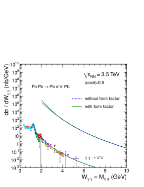
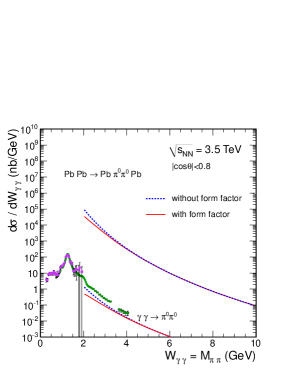
Figure 12: The nuclear (upper lines) and elementary (lower lines) cross section as a function of photon–photon subsystem energy $W_{\gamma\gamma}$ in the b-space EPA within the BL pQCD approach for the elementary cross section with Wu-Huang distribution amplitude. The angular ranges in the figure caption correspond to experimental cuts.

2.6 Exclusive production of $\rho^{0}\rho^{0}$ pairs

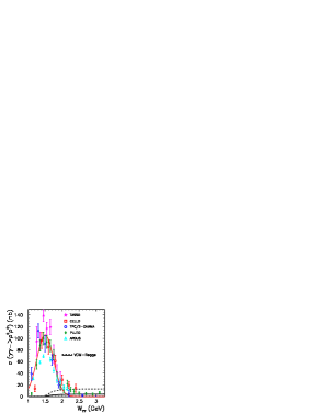
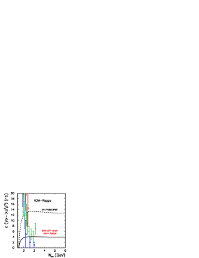
Figure 13: Elementary cross section for $\gamma\gamma\to\rho^{0}\rho^{0}$ reaction. The fit to the experimental data is shown in the left panel and our predictions for the high energy in the right panel.

At low energies one observes a huge enhancement of the cross section for the elementary process $\gamma\gamma\to\rho^{0}\rho^{0}$ (see left panel of Fig.13). In the right panel we show predictions of a simple Regge-VDM model with parameters adjusted to the world hadronic data. More details about our model can be found in our original paper [4].

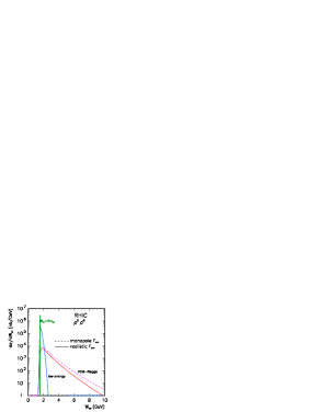
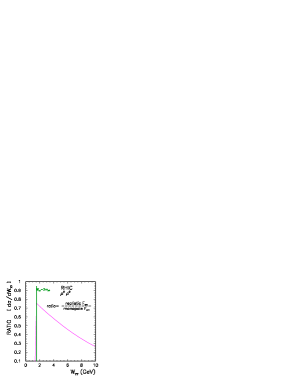
Figure 14: Distribution in the $\rho^{0}\rho^{0}$ invariant mass

In Fig.14 we show distribution in $\rho^{0}\rho^{0}$ invariant mass (left panel) and the ratio of the cross section for realistic and monopole form factors.

2.7 Some comments and outlook

We have presented some examples of processes that could be soon studied at RHIC or LHC. In all cases we have obtained measurable cross sections. We have pointed out that the inclusion of realistic charge form factor is necessary to obtain realistic particle distributions.

Measurements of the processes discussed here are not easy as one has to assure exclusivity of the process, i.e., it must be checked that there are no other particles than that measured in central detectors. In all cases fissibilty studies, including Monte Carlo simulations, are required.

In the close future one may expect results for two-pion and single vector mesons production from LHC experiments. Exclusive production of one or two pairs of charged leptons should be feasible too.

Acknowledgments Some of the results presented here were obtained in collaboration with Wolfgang Schäfer, Valerij Serbo and Magno Machado.

References

References

-
[1]
Budnev V M et al. 1975
Phys. Rep. 15 4
Bertulani C A, Baur G 1988 Phys. Rep. 163 299
Baur G, Hencken K, Trautmann D, Sadovsky S and Kharlov Y 2002 Phys. Rep. 364 259
Bertulani C A, Klein S and Nystrand J 2005 J Ann. Rev. Nucl. Part. Sci.55 271
Baltz A et al. 2008, Phys. Rep. 458 1 - [2] Kłusek-Gawenda M and Szczurek A 2010 Phys. Rev. C 82 014904
- [3] Kłusek-Gawenda M, Szczurek A, Machado M and Serbo V 2011 Phys. Rev. C 83 024903
- [4] Kłusek M, Schäfer W and Szczurek A 2009 Phys. Lett. B 674 92
- [5] Kłusek-Gawenda M and Szczurek A 2011, Phys. Lett. B 700 322
- [6] Łuszczak M and Szczurek A 2009 Phys. Lett. B 700 116
- [7] Jackson J D 1975, Classical Electrodynamics, 2nd ed. (Wiley, New York), p. 722
- [8] Hencken K, Trautmann D and Baur G 1994 Phys. Rev. A 49 1584
- [9] Barrett R C and Jackson D F 1977 Nuclear Sizes and Structure, (Clarendon Press, Oxford)
- [10] de Vries H, de Jager C W and de Vries C 1987 Atomic Data and Nuclear Data Tables 36 495
- [11] Baur G and Bertulani C A 1987 Phys. Rev. C 35 836
- [12] Hencken K, Trautmann D and Baur G 1999 Phys. Rev. C 59 841
-
[13]
Ivanov D Yu, Schiller A and Serbo V G 1999
Phys. Lett. B 454 155
Henecken K, Kuraev E A and Serbo V G 2007 Phys. Rev. C 75 034903
Jentschura U D, Hencken K and Serbo V G 2008 Eur. Phys. J. C 58 281
Jentschura U D and Serbo V G 2009 Eur. Phys. J. C 64 309 -
[14]
Baltz A 2008 Phys. Rev. Lett. 100 062302
Baltz A 2009 Phys. Rev. C 80 034901 - [15] Kniehl B A, Kotikov A V, Merebashvili Z V and Veretin O L 2009 Phys. Rev. D 79 114032
- [16] Timneanu N, Kwieciński J and Motyka L 2002 Eur. Phys. J. C 23 513
- [17] Szczurek A 2002 Eur. Phys. J. C 26 183
- [18] Gluck M, Reya E and Vogt A 1992 Phys. Rev. D 46 1973
- [19] Brodsky S J and Lepage G P 1981 Phys. Rev. D 24 1808
- [20] Ji C R and Amiri F 1990 Phys. Rev. D 42 3764
- [21] Brodsky S J and Lepage G P 1979 Phys. Lett. B 87 359
- [22] Efremov A V and Radyushkin A V 1980 Phys. Lett. B 94 245
- [23] Wu X G and Huang T 2010 Phys. Rev. D 82 034024
- [24] Chernyak V L and Zhitnitsky A R 1982 Nucl. Phys. B 201 492
-
[25]
Diehl M, Kroll P and Vogt C 2002
Phys. Lett. B 532 99
Diehl M and Kroll P 2010 Phys. Lett. B 683 165 - [26] Szczurek A and Speth J 2003 Eur. Phys. J. A 18 445