Influence Blocking Maximization in Social Networks
under the Competitive Linear Threshold Model  
 
Technical Report

Abstract

In many real-world situations, different and often opposite opinions, innovations, or products are competing with one another for their social influence in a networked society. In this paper, we study competitive influence propagation in social networks under the competitive linear threshold (CLT) model, an extension to the classic linear threshold model. Under the CLT model, we focus on the problem that one entity tries to block the influence propagation of its competing entity as much as possible by strategically selecting a number of seed nodes that could initiate its own influence propagation. We call this problem the influence blocking maximization (IBM) problem. We prove that the objective function of IBM in the CLT model is submodular, and thus a greedy algorithm could achieve $1-1/e$ approximation ratio. However, the greedy algorithm requires Monte-Carlo simulations of competitive influence propagation, which makes the algorithm not efficient. We design an efficient algorithm CLDAG, which utilizes the properties of the CLT model, to address this issue. We conduct extensive simulations of CLDAG, the greedy algorithm, and other baseline algorithms on real-world and synthetic datasets. Our results show that CLDAG is able to provide best accuracy in par with the greedy algorithm and often better than other algorithms, while it is two orders of magnitude faster than the greedy algorithm.

Keywords: influence blocking maximization, competitive linear threshold model, social networks

1 Introduction

With the increasing popularity of online social and information networks such as Facebook, Twitter, LinkedIn, etc., many researchers have studied diffusion phenomenon in social networks, which includes the diffusion of news, ideas, innovations, adoption of new products, etc. We generally refer to such diffusions as influence diffusion or propagation. One topic in influence diffusion that has been extensively studied is influence maximization [14, 15, 16, 19, 6, 5, 25, 7]. Influence maximization is the problem of selecting a small set of seed nodes in a social network, such that its overall influence coverage is maximized, under certain influence diffusion models. Popular influence diffusion models include the independent cascade (IC) model and the linear threshold (LT) model, which was first summarized by Kempe et al. in [14] based on prior research in social network analysis and particle physics. Both IC and LT models are stochastic models characterizing how influence are propagated throughout the network starting from the initial seed nodes.

However, all of the above research works only study the diffusion of a single idea in the social networks. In reality, it is often the case that different and often opposite information, ideas and innovations are competing for their influence in the social networks. Such competing influence diffusion could range from two competing companies engaging in two marketing campaigns trying to grab people’s attentions, or two political candidates of the opposing parties trying to influence their voters, to government authorities trying to inject truth information to fight with rumors spreading in the public, and so on.

Motivated by the above scenarios, several recent studies have looked into competitive influence diffusion and its corresponding influence maximization problems [1, 17, 21, 24, 2, 3, 4]. Most of them propose some extensions to the existing influence diffusion models to incorporate competitive influence diffusion, and then either focus on the influence maximization problem for one of the competing parties, or study the game theoretic aspects of competitive influence diffusion (see Section 2 for more details on these related works). In this paper, we concentrate on the problem of how to block the influence diffusion of an opposing party as much as possible. For example, when there is a negative rumor spreading in the social network about a company, the company may want to react quickly by selecting seed nodes to inject positive opinions about the company to fight against the negative rumor. Similar situations could occur when a political candidate tries to stop a negative rumor about him or her, or when government or public officials try to stop erroneous rumors about public health and safety, terrorist threat, etc. We call the problem of selecting positive seed nodes in a social network to minimize the effect of negative influence diffusion, or to maximize the blocking effect on negative influence, the influence blocking maximization (IBM) problem.

We study the IBM problem under a competitive linear threshold (CLT) model, which we extend naturally from the classic linear threshold model and is similar to a model proposed independently in [2]. We prove that the objective function of IBM under the CLT model is monotone and submodular, which means a standard greedy algorithm can achieve an approximation ratio of $1-1/e-\epsilon$ to the optimal solution, where $\epsilon$ is any positive number. However, the greedy algorithm requires Monte-Carlo simulations of competitive influence diffusion, which becomes very slow for large networks, if we want to keep $\epsilon$ above small. For example, in our simulation, for a network with 6.4k nodes, the greedy algorithm takes more than 8 hours to finish. This is especially problematic for the IBM problem, since blocking influence diffusion usually requires very swift decisions before the negative influence propagates too far. To address the efficiency issue, we utilize the efficient computation property of the LT model for directed acyclic graphs (DAGs), and design an efficient heuristic CLDAG for the IBM problem under the CLT model. Because of the complex interaction in the competitive influence diffusion under the CLT model, we need a carefully designed dynamic programming method for influence computation in our CLDAG algorithm. To test the efficiency and effectiveness of our CLDAG algorithm, we conduct extensive simulations on three real-world networks as well as synthetic networks. We compare the performance of CLDAG with the greedy algorithm and other heuristic algorithms. Our results show that (a) comparing with the greedy algorithm, our CLDAG algorithm achieves matching influence blocking effect while it runs two orders of magnitude faster; and (b) comparing with other heuristics such as degree-based heuristics, our algorithm consistently performs well and is often better than the other heuristics with a significant margin.

To the best of our knowledge, our work is the first to study the IBM problem under the competitive linear threshold model. The study closest to our work is the one in [3], but they study the IBM problem under an extension of the independent cascade model, and due to the issue of non-submodularity, their study only works for a restricted extention to the IC model that is less natural. Moreover, their work does not address the efficiency issue, which is vital to influence blocking maximization.

The rest of the paper is organized as follows. We discuss related works in Section 2. In Section 3, we specify the competitive linear threshold model. In Section 4, we define the influence blocking maximization problem, show that it is NP-hard, and prove its submodularity under the CLT model. We describe our CLDAG algorithm in Section 5, and then provide our experimental evaluation results in Section 6. We conclude the paper with discussions in Section 7.

2 Related Work

Independent cascade model and linear threshold model are two extensively studied influence diffusions models originally summarized by Kempe et al. [14], based on earlier works of [11, 23, 10]. Kempe et al. prove that the generalized versions of these two models are equivalent [14]. Based on the IC and LT model, Kempe et.al  [14, 15] propose a greedy algorithm to solve the influence maximization problem (brought about by Richardson [22]) to maximize the spreading of a single piece of ideas, innovations, etc. under these two models. Many follow-up studies propose alternative heuristics and try to solve the influence maximization problem more efficiently [16, 19, 6, 5, 7, 25]. In terms of efficient algorithm design, our work follows the idea in [5, 7] of finding efficient local graph structures to speed up the computation. In particular, our CLDAG algorithm is similar to the LDAG algorithm of [7], which is also based on the DAG structure, but our CLDAG algorithm is novel in dealing with competitive influence diffusion using the dynamic programming method.

Recently, there are a number of studies on competitive influence diffusion [1, 17, 21, 24, 2, 3, 4]. Bharathi et al, extend the IC model to model competitive influence [1], but they only provide a polynomial approximation algorithm for trees. Kostka et al. study competitive rumor spreading [17] on a more restricted model than IC and LT, and focused on showing the hardness of computing the optimal solution for the two competing parties. Pathak et al. study a model of multiple cascades [21], which is an extension of a different diffusion model called the voter model [8, 13], even though they claim it to be a generalization of the linear threshold model. They only study model dynamics and do not address the influence maximization problem. Trpevski et al. [24] propose another competitive rumor spreading model based on the epidemic model of SIS and study the dynamics in several classes of graphs, and they do not address the issue of influence maximization either. Borodin et.al [2] extend the LT model in several different ways to model competitive influence diffusion, one of which is essentially our CLT model except for a different tie-breaking rule. However, they only study the influence maximization problem, not the influence blocking maximization. In particular, they show that influence maximization in the CLT model is not submodular, which is an interesting contrast to our result that influence blocking maximization under the CLT model is submodular. We provide some reason in Section 7 on why there is such a subtle difference. The work of Budak et al. [3] is the only one we found that studies influence blocking maximization (they call it eventual influence limitation), but they study this problem under an extension of the IC model. They show that the general extension of the IC model in which positive influence and negative influence has a separate set of parameters (same as the case in our CLT model) is not submodular, and thus to achieve submodularity they have to restrict the model such that positive propagation probability is $1$ or is the same as negative propagation probability, which limits the expressiveness of the model. Moreover, they only study the greedy algorithm and some simple heuristics, and do not provide efficient and scalable solution that maintains good accuracy at the same time. Finally the work of [4] studies negative opinions emerging from poor product or service qualities, not generated by competitors. They study positive influence maximization under an extension to the IC model, and thus different from our study on blocking negative influence under the extension of the LT model. The efficient influence maximization algorithm in [4] also uses dynamic programming, which bears some resemblance to our work.

3 Competitive Linear Threshold Model

Kempe et al. proposed the linear threshold model in [14] as a stochastic model to address information cascade in a network. In this model, a social network is considered as a directed graph $G=(V,E)$, where $V$ is the set of vertices representing individuals and $E$ is the set of directed edges representing influence relationships among individuals. Each edge $(u,v)\in E$ has a weight $w_{uv}\geq 0$, indicating the importance of $u$ in influencing $v$. For convenience, for any $(u,v)\not\in E$, $w_{uv}=0$. For each $v\in V$, we have $\sum_{u\in V}w_{uv}\leq 1$. Each vertex $v$ picks an independent threshold $\theta_{v}$ uniformly at random from $[0,1]$. Each vertex is either inactive or active, and once it is active, it stays active forever. The diffusion process unfolds in discrete time steps. At step $0$ a seed set $S\subseteq V$ is activated while all other vertices are inactive. At any later step $t>0$, a vertex $v$ is activated if and only if the total weight of its active in-neighbors exceeds its threshold $\theta_{v}$, that is $\sum_{u\in S_{t-1}}w_{uv}\geq\theta_{v}$, where $S_{t-1}\subseteq V$ is the set of active vertices by time $t-1$, with $S_{0}=S$.

We now extend the LT model to incorporate competitive influence diffusion. The idea is that we allow each vertex to be positively activated or negatively activated, each of which is determined by concurrent positive diffusion and negative diffusion, respectively. In the case that a vertex is both positively activated and negatively activated in the same step, then negative activation dominates the result.

More precisely, we define competitive linear threshold (CLT) model as an extension to the LT model in the following way. Each vertex has three states, inactive, +active, and -active, and it does not change state once it becomes +active or -active. Each edge $(u,v)$ has two weights, positive weight $w_{uv}^{+}$ and negative weight $w_{uv}^{-}$. We can also think of it as $(u,v)$ splitting into two virtual edges, one positive edge propagating positive influence and one negative edge propagating negative influence. Each vertex $v$ picks two independent thresholds uniformly at random from $[0,1]$, one positive threshold $\theta^{+}_{v}$ and one negative threshold $\theta^{-}_{v}$. At step $0$, there are two disjoint seed sets, the positive seed set $P_{0}$ and the negative seed set $N_{0}$. At each step $t$, positive influence and negative influence propagate independently as in the original LT model, using positive weights/thresholds and negative weights/thresholds, respectively. If a vertex $v$ is activated only by positive diffusion (or resp. negative diffusion), then $v$ becomes +active (or resp. -active). If in step $t$ $v$ is activated by both positive diffusion and negative diffusion, then negative diffusion dominates and $v$ becomes -active. The negative dominance rule reflects the negativity bias phenomenon well studied in social psychology, and matches the common sense that rumors are usually hard to fight with.

The CLT model defined here is essentially the same as the separate threshold model of [2], except that we use the negative dominance as the tie-breaking rule, while they use the random rule — +active and -active status are picked uniformly at random. We comment that the difference in the tie-breaking rule is not essential for our study: the submodularity property still holds and our algorithm can be properly adapted for the random tie-breaking rule.

4 Influence Blocking Maximization Problem

In this section, we first define the influence blocking maximization (IBM) problem, then show that IBM under the CLT model is NP-hard, and finally prove that the objective function of IBM is monotone and submodular, which leads to a greedy approximation algorithm.

4.1 Problem definition.

Informally, the IBM problem is an optimization problem in which given a graph $G=(V,E)$, its positive and negative edge weights, a negative seed set $N_{0}$, and a positive integer $k$, we want to find a positive seed set $S$ of size at most $k$ such that the expected number of negatively activated nodes is minimized, or equivalently, the reduction in the number of negatively activated nodes is maximized.

More precisely, let $\vec{\theta}^{+}$ and $\vec{\theta}^{-}$ be the vector of positive thresholds and negative thresholds, respectively, for all vertices in $G$. According to the CLT model, they are drawn from the probability space $[0,1]^{|V|}$ uniformly at random. When $\vec{\theta}^{+}$ and $\vec{\theta}^{-}$ are fixed, all randomness in the CLT model is fixed. Let ${\it IBS}(S,N_{0}\ |\ \vec{\theta}^{+},\vec{\theta}^{-})$ be the set of nodes $v$ in $G$ such that under thresholds $\vec{\theta}^{+}$ and $\vec{\theta}^{-}$, $v$ is negatively activated if $N_{0}$ is the negative seed set and positive seed set is empty, while $v$ is not negatively activated if $N_{0}$ is the negative seed set and $S$ is the positive seed set. Thus this set represents the set of nodes that have been blocked from negative influence, and IBS stands for influence blocking set. Since we always use $N_{0}$ as the negative seed set, we will omit $N_{0}$ from the notation for simplicity. When the context is clear, we may also omit $\vec{\theta}^{+}$ and $\vec{\theta}^{-}$ and only use ${\it IBS}(S)$ to represent the influence blocking set. We define negative influence reduction (NIR) of a positive seed set $S$, denoted as $\sigma_{{\it NIR}}(S)$, to be the expected value of the size of ${\it IBS}(S\ |\ \vec{\theta}^{+},\vec{\theta}^{-})$, with expectation taken over all $\vec{\theta}^{+}$’s and $\vec{\theta}^{-}$’s, that is,

$$\sigma_{{\it NIR}}(S)=E_{\vec{\theta}^{+},\vec{\theta}^{-}}(|{\it IBS}(S\ |\ \vec{\theta}^{+},\vec{\theta}^{-})|).$$

Then the influence blocking maximization is the problem of finding a positive seed set $S$ of size at most $k$ that maximizes $\sigma_{{\it NIR}}(S)$, i.e., computing

$$P^{*}=\arg\max_{|S|\leq k}\sigma_{{\it NIR}}(S).$$

We first show that the exact problem of IBM is NP-hard.

Theorem 4.1

Under the CLT model, IBM problem is NP-hard.

• By a reduction from the vertex cover problem. The full NP-hardness proof in presented in Appendix. $\Box$

4.2 Submodularity of $\sigma_{{\it NIR}}(S)$ and the greedy approximation algorithm.

To overcome the NP-hardness result of Theorem 4.1, we look for approximation algorithms. The submodularity of set function $\sigma_{{\it NIR}}(S)$ provides a good way to obtain an apporiximation algorithm for the IBM problem. We say that a set function $f(S)$ with domain $2^{V}$ is submodular if for all $S\subseteq T\subseteq V$, and $x\not\in T$, we have $f(S\cup\{x\})-f(S)\geq f(T\cup\{x\})-f(T)$. Intuitively, submodularity of $f$ means $f$ has the diminishing marginal return property. Moreover, we say that $f$ is monotone if for all $S\subseteq T\subseteq V$, $f(S)\leq f(T)$.

We now show that $\sigma_{{\it NIR}}(S)$ is monotone and submodular. We follow the general methodology as in [14] for the proof, but our proof is more involved because of the complexity of our CLT model and the IBM problem. We first construct an equivalent random process, and then use this random process to prove the result.

From the original graph $G=(V,E)$ with positive and negative weights, we construct a random live-path graph $G_{X}$ as follows. For each $v\in V$, we randomly pick one positive in-edge $(u,v)$ with probability $w_{uv}^{+}$, and with probability $1-\sum_{u\in V}w_{uv}^{+}$ no positive in-edge is selected; we also randomly pick one negative in-edge $(u,v)$ with probability $w_{uv}^{-}$, and with probability $1-\sum_{u\in V}w_{uv}^{-}$ no negative in-edge is selected. Let $G^{+}$ be the subgraph of $G_{X}$ consisting of only positive edges, and let $G^{-}$ be the subgraph of $G_{X}$ consisting of only negative edges. Given a positive seed set $P_{0}$ and a negative seed set $N_{0}$, define $d_{G^{+}}(P_{0},v)$ to be the shortest graph distance from any node in $P_{0}$ to $v$ only through the positive edges, and $d_{G^{-}}(N_{0},v)$ to be the shortest graph distance from any node in $N_{0}$ to $v$ only through the negative edges. The above distance could be $\infty$ if no such path exists. Then in the random live-path graph, we say a node $v$ is +active if $d_{G^{+}}(P_{0},v)<\infty$ and $d_{G^{+}}(P_{0},v)<d_{G^{-}}(N_{0},v)$, and $v$ is -active if $d_{G^{-}}(N_{0},v)<\infty$ and $d_{G^{-}}(N_{0},v)\leq d_{G^{+}}(P_{0},v)$. The following lemma shows that the positive and negative activation sets generated by the above random process is equivalent to the corresponding one generated by the CLT model.

Lemma 4.1

For a given positive seed set $P_{0}$ and negative seed set $N_{0}$, the distribution over +active sets and -active sets is identical in the following two definitions.

1. distribution obtained by running CLT process,

2. distribution obtained from reachability defined above in the live-path graph.

• The activation process under the CLT model consists of several iterations. In each iteration, some nodes change from inactive to +active or -active. Thus we first define $A_{t}^{+}$ to be the set of +active nodes at the end of iteration $t$ and $A_{t}^{-}$ as the set of -active nodes at the end of iteration $t$, for $t=0,1,2...$. Here we consider a node $v$ which has not been activated by the end of iteration $t$, namely $v\not\in A_{t}^{+}\cup A_{t}^{-}$. Thus the probability $v$ becomes +active in iteration $t+1$ equals to the chance that the positive influence weights in $A_{t}^{+}\backslash A_{t-1}^{+}$ push it over the positive threshold while the negative influence weights is still less than the negative threshold. The above probability under the condition that neither node $v$’s negative nor positive threshold is exceeded already by step $t$ is:

  $$\frac{(\sum_{u\in A_{t}^{+}\backslash A_{t-1}^{+}}w^{+}_{uv})(1-\sum_{u\in A_{t}^{-}\backslash A_{t-1}^{-}}w^{-}_{uv})}{(1-\sum_{u\in A_{t-1}^{+}}w^{+}_{uv})(1-\sum_{u\in A_{t-1}^{-}}w^{-}_{uv})}.$$

  Similarly we can get the probability that node $v$ becomes -active in iteration $t+1$ given than node $v$ is inactive from iteration $0$ to $t$. The probability is:

  $$\frac{\sum_{u\in A_{t}^{-}\backslash A_{t-1}^{-}}w^{-}_{uv}}{(1-\sum_{u\in A_{t-1}^{+}}w^{+}_{uv})(1-\sum_{u\in A_{t-1}^{-}}w^{-}_{uv})}.$$

On the other hand, we consider the above discussed probability when using the random live-path graph. We start from seed set $P_{0}$ and $N_{0}$ and called them ${B_{0}^{+}}$ and ${B_{0}^{-}}$, respectively. For each $t=1,2,\ldots$, we define ${B_{t}^{-}}$ to be the set containing any $v\not\in{B_{t-1}^{+}}\cup{B_{t-1}^{-}}$ such that $v$ has one in-edge from some node in ${B_{t-1}^{-}}$; we define ${B_{t}^{+}}$ to be the set containing any $v\not\in{B_{t-1}^{+}}\cup{B_{t-1}^{-}}$ such that $v$ has one in-edge from some node in ${B_{t-1}^{+}}$ but no in-edge from any node in ${B_{t-1}^{-}}$.

By the definition of the random live-path graph, the probability that a node $v$ is in $B_{t+1}^{+}\setminus B_{t}^{+}$ conditioned on that $v$ is not in ${B_{t}^{+}}\cup{B_{t}^{-}}$ is

$$\frac{(\sum_{u\in{B_{t}^{+}}\backslash{B_{t-1}^{+}}}w^{+}_{uv})(1-\sum_{u\in{B_{t}^{-}}\backslash{B_{t-1}^{-}}}w^{-}_{uv})}{(1-\sum_{u\in{B_{t-1}^{+}}}w^{+}_{uv})(1-\sum_{u\in{B_{t-1}^{-}}}w^{-}_{uv})}.$$

Similarly, the probability that a node $v$ is in $B_{t+1}^{-}\setminus B_{t}^{-}$ conditioned on that $v$ is not in ${B_{t}^{+}}\cup{B_{t}^{-}}$ is

$$\frac{\sum_{u\in{B_{t}^{-}}\backslash{B_{t-1}^{-}}}w^{-}_{uv}}{(1-\sum_{u\in{B_{t-1}^{+}}}w^{+}_{uv})(1-\sum_{u\in{B_{t-1}^{-}}}w^{-}_{uv})}.$$

The above conditional probabilities are the same as derived from the CLT model. Since $A_{0}^{+}={B_{0}^{+}}$ and $A_{0}^{-}={B_{0}^{-}}$, by induction over the iterations, we reach at the conclusion that the random live-path graph model produces the same distribution over +active and -active sets as the CLT model. $\Box$

With the equivalence shown in Lemma 4.1, we now focus on showing the monotonicity and submodularity of negative influence reduction in the random live-path graph model. With a bit of abuse in notation, given a live-path graph $G_{X}$ and a negative seed set $N_{0}$, we also use ${\it IBS}(S)$ to denote the set of nodes in $V$ which would be -active if the positive seed set is empty but is not -active if the positive seed set is $S$. Then the negative influence reduction $\sigma_{{\it NIR}}(S)=E_{G_{X}}(|{\it IBS}(S)|)$.

Given a set $S$ and a node $u\not\in S$, we say that there is a unique path from $S$ to $u$ if there exists some path from a node in $S$ to $u$, and for any two paths from any two nodes in $S$ to $u$, one path must be a sub-path of the other. In addition, whenever we refer to the unique path from $S$ to $u$, we mean the unique shortest path from any node in $S$ to $u$. The following lemma shows a simple yet important property of the live-path graph that leads to the submodularity proof.

Lemma 4.2

In a live-path graph $G_{X}$, for any node $v$, there is a unique positive path from some node in the positive seed set $S$ to $v$, if $d_{G^{+}}(S,v)<\infty$, and there is a unique negative path from some node in the negative seed set $N_{0}$ to $v$, if $d_{G^{-}}(N_{0},v)<\infty$.

• This is obvious because each node has at most one positive in-edge and one negative in-edge. $\Box$

Then we use next two lemmas to give the sufficient and necessary conditions for $v\in{\it IBS}(S)$ and $v\in{\it IBS}(T\cup\{u\})\verb"\"{\it IBS}(T)$ in a live-path graph $G_{X}$.

Lemma 4.3

The sufficient and necessary condition for $v\in{\it IBS}(S)$ is:

1. There exist a unique negative path in $G^{-}$ from node set $N_{0}$ to $v$, namely $d_{G^{-}}(N_{0},v)<\infty$, and

2. there exists at least one node $u$ in the unique negative path, such that $d_{G^{+}}(S,u)<d_{G^{-}}(N_{0},u)$.

• Lemma 4.3 is an obvious derivation from the definition of ${\it IBS}(S)$ and Lemma 4.2. $\Box$

Lemma 4.4

The sufficient and necessary condition for $u\in{\it IBS}(T\cup\{v\})\verb"\"{\it IBS}(T)$ is:

1. There exists a unique negative path from $N_{0}$ to $u$,

2. there exists at least one node $w$ on the unique negative path from $N_{0}$ to $u$, such that $d_{G^{+}}(T\cup\{v\},w)<d_{G^{-}}(N_{0},w)$, and

3. for all node $t$ on the unique negative path from $N_{0}$ to $u$, there holds that $d_{G^{+}}(T,t)\geq d_{G^{-}}(N_{0},t)$.

• The above conditions 1 and 2 are direct conclusions of Lemma 4.3 on $u\in{\it IBS}(T\cup\{v\})$. Condition 3 is the direct derivation of Lemma 4.3 on $u\not\in{\it IBS}(T)$. $\Box$

Lemma 4.5

The cardinality set function $|{\it IBS}(S)|$ for a live-path graph $G_{X}$ is monotone and submodular.

• We first prove the monotonicity of $|{\it IBS}(S)|$, namely for any node $u\in V\backslash(S\cup N_{0})$ and subset $S\subseteq V$, $|{\it IBS}(S)|\leq|{\it IBS}(S\cup\{u\})|$. We prove the result by showing that ${\it IBS}(S)\subseteq{\it IBS}(S\cup\{u\})$. Consider any node $v\in{\it IBS}(S)$. By Lemma 4.3, we have $d_{G^{-}}(N_{0},v)<\infty$, and there exists a node $w$ in the unique negative path from $N_{0}$ to $v$ such that $d_{G^{+}}(S,w)<d_{G^{-}}(N_{0},w)$. It is also clear that $d_{G^{+}}(S\cup\{u\},w)\leq d_{G^{+}}(S,w)$. Thus, we have $d_{G^{+}}(S\cup\{u\},w)<d_{G^{-}}(N_{0},w)$, and by Lemma 4.3, $v\in{\it IBS}(S\cup\{u\})$.

We then prove submodularity of $|{\it IBS}(S)|$ by showing: For any subset $S\subseteq V,T\subseteq V,S\subseteq T$ and $v\in V\backslash(T\cup N_{0})$,

$${\it IBS}(T\cup\{v\})\verb"\"{\it IBS}(T)\subseteq{\it IBS}(S\cup\{v\})\verb"\"{\it IBS}(S).$$

Given any $u\in{\it IBS}(T\cup\{v\})\verb"\"{\it IBS}(T)$, we prove that $u\in{\it IBS}(S\cup\{v\})\verb"\"{\it IBS}(S)$ by showing all three conditions in Lemma 4.4 are satisfied. The satisfaction of 1 is obvious, since $d_{G^{-}}(N_{0},u)$ doesn’t change. As for condition 2, we know that there exists a node $w$ on the unique negative path from $N_{0}$ to $u$, $d_{G^{+}}(T\cup\{v\},w)<d_{G^{-}}(N_{0},w)$ and for all node $t$ on path from $N_{0}$ to $u$, $d_{G^{+}}(T,t)\geq d_{G^{-}}(N_{0},t)$. Then for node $w$, $d_{G^{+}}(T\cup\{v\},w)<d_{G^{-}}(N_{0},w)\leq d_{G^{+}}(T,w)$, which implies that $d_{G^{+}}(T\cup\{v\},w)=d_{G^{+}}(v,w)$. According to Lemma 4.2, the positive influence can reach node $w$ only in the unique positive path from $v$ to $w$. Thus $d_{G^{+}}(S\cup\{v\},w)=d_{G^{+}}(v,w)=d_{G^{+}}(T\cup\{v\},w)<d_{G^{-}}(N_{0},w)$. Then consider condition 3. For any node $t$ in the unique negative path from $N_{0}$ to $u$, $d_{G^{+}}(T,t)\geq d_{G^{-}}(N_{0},t)$. Since $S\subseteq T$, it is easy to verify that $d_{G^{+}}(S,t)\geq d_{G^{+}}(T,t)$. Therefore, $d_{G^{+}}(S,t)\geq d_{G^{-}}(N_{0},t)$ and condition 3 also holds. $\Box$

Theorem 4.2

For the CLT model, $\sigma_{{\it NIR}}(S)$ is monotone and submodular.

• By Lemma 4.1, we know that the CLT model is equivalent to the random live-path graph model. By Lemma 4.5, we know that for each live-path graph, the size of the influence blocking set is monotone and submodular. Since $\sigma_{{\it NIR}}(S)=E_{G_{X}}(|{\it IBS}(S)|)$ and any convex combinations of monotone and submodular functions are still monotone and submodular, we know that $\sigma_{{\it NIR}}(S)$ is monotone and submodular. $\Box$

We have shown that the influence blocking maximization problem under CLT model is monotone and submodular. Moreover, we have $\sigma_{{\it NIR}}(\emptyset)=0$. Then by the famous result in [20], the greedy algorithm given in Algorithm 1 achieves $1-1/e$ approximation of the optimal solution. The algorithm simply selects seed nodes one by one, and each time it always selects the node that provides the largest marginal gain to the negative influence reduction.

Algorithm 1 Greedy($k$,$N_{0}$)

1:  initialize $S=\emptyset$

2:  for $i=1$ to $k$ do

3:     select $u=arg\max_{v\in V\backslash(N_{0}\cup S)}(\sigma_{{\it NIR}}(S\cup\{v\}))$

4:     $S=S\cup\{u\}$

5:  end for

6:  return $S$

However, the greedy algorithm requires the evaluation of $\sigma_{{\it NIR}}(S)$, which cannot be done efficiently. The standard way of using Monte-Carlo simulations to estimate $\sigma_{{\it NIR}}(S)$ is slow, especially when we need to simulate the interfering propagation of competing influences. Even with powerful optimization method such as the lazy forward optimization of [18] or more advanced approach in [6], greedy algorithm still takes unacceptable long time for large graphs of more than $10k$ nodes. We address this efficiency issue in the next section with our new algorithm CLDAG.

5 CLDAG Algorithm for the IBM Problem

Motivated by the extremely low efficiency of greedy algorithm, we try to tackle this problem with an innovative heuristic approach proposed by Chen et al. in [5, 7]. This heuristic is characterized (a) by restricting influence computation of a node $v$ to its local area to reduce computation cost; and (b) by carefully selecting a local graph structure for $v$ to allow efficient and accurate influence computation for $v$ under this structure. For the LT model, Chen et al. use a local directed acyclic graph (LDAG) structure [7], because it allows linear computation of influence in a LDAG, as well as efficient construction of LDAGs using an algorithm similar in style to the Dijkstra’s shortest path algorithm. We repeat the LDAG construction algorithm of [7] in our Algorithm 2 for completeness. We use $N_{in}(x)$ to denote the set of in-neighbors of node $x$. The $\theta$ in the algorithm is a threshold from $0$ to $1$ controlling the size of the LDAG — the smaller the $\theta$, the larger the LDAG. The algorithm includes a node $x$ only if its influence to $v$ through the LDAG edges are at least $\theta$. The key update step in line 7 is based on the important linear relationship of activation probabilities in DAG structures shown in [7], and repeated below:

(5.1) $${\it ap}(x)=\sum_{u\in N_{in}(x)}w_{ux}\cdot{\it ap}(u),$$

where ${\it ap}(x)$ is the activation probability of node $x$ when a seed set is fixed.

Algorithm 2 Find-LDAG($G$,$v$,$\theta$),compute LDAG for $v$ with threshold $\theta$

1:  $X=\emptyset$;$Y=\emptyset$;$\forall v\in V,{\it Inf}(u,v)=0$;${\it Inf}(v,v)=1$

2:  while $\max_{v\in V\setminus X}{\it Inf}(u,v)\geq\theta$ do

3:     $x=arg\max_{u\in V\setminus X}{\it Inf}(u,v)$

4:     $Y=Y\cup\{(x,u)|u\in X\}$

5:     $X=X\cup\{x\}$

6:     for each node $u\in N_{in}(x)$ do

7:         ${\it Inf}(u,v)\,\mathrm{+=}\ w_{ux}*{\it Inf}(x,v)$

8:     end for

9:  end while

10:  return $D=(X,Y,w)$ as the LDAG($v$,$\theta$)

However, for the CLT model, negative and positive influence are propagated concurrently in the network and interfere with each other. Thus we need to adjust our LDAG construction and influence computation for the CLT model. First, for each node $v$, we use Algorithm 2 to construct two LDAGs, ${\it LDAG}^{+}(v)$ and ${\it LDAG}^{-}(v)$, using positive weights and negative weights respectively. Second, we need to carefully compute the positive activation probability ${\it ap}^{+}(v)$ and negative activation probability ${\it ap}^{-}(v)$, for any node $v$ under the CLT model, assuming positive and negative influence are propagated through ${\it LDAG}^{+}(v)$ and ${\it LDAG}^{-}(v)$ respectively. This involves a dynamic programming formulation detailed in the following subsection.

5.1 Influence computation.

We propose a dynamic programming method, Inf-CLDAG, to compute the exact activation probability of the central node $v$ in local structure ${\it LDAG}^{+}(v)$ and ${\it LDAG}^{-}(v)$. Under the CLT model, two opposite influence diffusions correlate together when disseminating in the graph, which makes it more tricky than the computation in the origin LT model. In this case, number of steps taken to activate a node becomes an important factor that must be taken into consideration when computing the cascade result.

For the following computation, we assume that the positive seed set $S$ and the negative seed set $N_{0}$ are fixed, and influence to $v$ only diffuses in ${\it LDAG}^{+}(v)$ and ${\it LDAG}^{-}(v)$. For the IBM problem, we want to compute the negative influence reduction under the positive seed set $S$. It is essentially a computation of negative influence coverage, which is given by $\sum_{v}{\it ap}^{-}(v)$.

Let $P^{+}(v,t)$ be the probability that the summation of the positive weights of in-edges of positively activated neighbors of node $v$ exceeds its positive threshold exactly at time $t$, and similar for $P^{-}(v,t)$. Let ${\it ap}^{+}(v,t)$ be the probability that $v$ becomes positively activated exactly at time $t$, and similar for ${\it ap}^{-}(v,t)$. Then we have ${\it ap}^{+}(v)=\sum_{t}{\it ap}^{+}(v,t)$ and ${\it ap}^{-}(v)=\sum_{t}{\it ap}^{-}(v,t)$. We now show how to compute ${\it ap}^{+}(v,t)$ and ${\it ap}^{-}(v,t)$.

By the definition of the CLT model, we have the following for any $v\in V\setminus(S\cup N_{0})$ and any $t\geq 1$:

(5.2) $$P^{+}(v,t)=\sum_{u\in{\it LDAG}^{+}(v)}w^{+}_{uv}{\it ap}^{+}(u,t-1),$$

(5.3) $$P^{-}(v,t)=\sum_{u\in{\it LDAG}^{-}(v)}w^{-}_{uv}{\it ap}^{-}(u,t-1),$$

(5.4) $${\it ap}^{+}(v,t)=P^{+}(v,t)(1-\sum_{k=0}^{t}P^{-}(v,k)),$$

(5.5) $${\it ap}^{-}(v,t)=P^{-}(v,t)(1-\sum_{k=0}^{t-1}P^{+}(v,k)).$$

Equations (5.2) and (5.3) can be reached by subtracting the probability that the summation of the weights of in-edges of activated neighbors of node $v$ exceeds threshold in any round from $0$ to $t-1$ from the corresponding probability for rounds from $0$ to $t$. Equation (5.4) is derived from the fact that if a node $v$ becomes positively activated at round $t$, then exactly at round $t$ the summation of positive weights must exceed the positive threshold, while by round $t$ the summation of negative weights does not exceed the negative threshold (otherwise $v$ would be negatively activated). The case for Equation (5.5) is similar.

The boundary conditions of the above equations are (a) for $v\in S$, ${\it ap}^{+}(v,0)=1$,$P^{+}(v,0)=0$, $P^{+}(v,t)={\it ap}^{+}(v,t)=0$ for all $t\geq 1$, $P^{-}(v,t)={\it ap}^{-}(v,t)=0$ for all $t\geq 0$; (b) for $v\in N_{0}$, ${\it ap}^{-}(v,0)=1$,$P^{-}(v,0)=0$ $P^{-}(v,t)={\it ap}^{-}(v,t)=0$ for all $t\geq 1$, $P^{+}(v,t)={\it ap}^{+}(v,t)=0$ for all $t\geq 0$; and (c) for $v\not\in S\cup N_{0}$, $P^{+}(v,0)={\it ap}^{+}(v,0)=P^{-}(v,0)={\it ap}^{-}(v,0)=0$. From the above equations together with the boundary conditions, the dynamic programming algorithm can be applied to compute the exact activation probability for every node $v$. However, the naive implementation will take $O(m_{D}\ell_{D})$ time, where $m_{D}$ is the size of ${\it LDAG}^{+}(v)$ and ${\it LDAG}^{-}(v)$ and $\ell_{D}$ is the length of the longest path in ${\it LDAG}^{+}(v)$ and ${\it LDAG}^{-}(v)$. With a careful planning, as described below, we could reduce the time to $O(m_{D})$ instead.

Algorithm 3 provides the pseudocode for our algorithm Inf-CLDAG, which computes the negative influence ${\it ap}^{-}(v)$ to $v$ from positive seed set $S$ and negative seed set $N_{0}$, through $v$’s LDAGs ${\it LDAG}^{+}(v)$ and ${\it LDAG}^{-}(v)$. The key feature of the algorithm is the alternating breadth-first-search (BFS) traversal on ${\it LDAG}^{-}(v)$ and ${\it LDAG}^{+}(v)$. Starting from the negative seed set we do one step BFS in ${\it LDAG}^{-}(v)$ and compute $P^{-}(x,1)$’s and ${\it ap}^{-}(x,1)$’s for those traversed nodes. We then do one step BFS in ${\it LDAG}^{+}(v)$ from the positive seeds, and compute $P^{+}(x,1)$’s and ${\it ap}^{+}(x,1)$’s for the traversed nodes. We then go back to ${\it LDAG}^{-}(v)$ to do one more layer of BFS and then go back to ${\it LDAG}^{+}(v)$ for one more layer of BFS, and so on. With this setup, we only need one BFS traversal of ${\it LDAG}^{+}(v)$ and ${\it LDAG}^{-}(v)$ to compute all ${\it ap}^{-}(u,t)$’s, and thus save the running time to $O(m_{D})$.

Algorithm 3 Inf-CLDAG($v,{\it LDAG}^{+}(v),{\it LDAG}^{-}(v),S,N_{0}$)

1:  $Q^{+}_{0}:=S\cap V({\it LDAG}^{+}(v))$

2:  $Q^{-}_{0}:=N_{0}\cap V({\it LDAG}^{-}(v))$

3:  initialize ${\it ap}^{+}(u,t),{\it ap}^{-}(u,t),P^{+}(u,t),P^{-}(u,t)$ for all $u$ and $t$ to $0$ or according to the boundary condition// can do initialization just when needed, so no extra time needed

4:  set $t=0$

5:  while $Q^{+}_{t}\neq\emptyset$ or $Q^{-}_{t}\neq\emptyset$ do

6:     for all node $u$ in $Q^{-}_{t}$ do

7:        for all node $x$ in ${\it LDAG}^{-}(v)$ and $w^{-}_{ux}\neq 0$ and $x\not\in S\cup N_{0}$ do

8:           add node $x$ into $Q^{-}_{t+1}$

9:           $P^{-}(x,t+1)=P^{-}(x,t+1)+w^{-}_{ux}{\it ap}^{-}(u,t)$

10:        end for

11:     end for

12:     for all node $x$ in $Q^{-}_{t+1}$ do

13:        ${\it ap}^{-}(x,t+1)=P^{-}(x,t+1)(1-\sum_{k=0}^{t}P^{+}(x,k))$

14:     end for

15:     for all node $u$ in $Q^{+}_{t}$ do

16:        for all node $x$ in ${\it LDAG}^{+}(v)$ and $w^{+}_{ux}\neq 0$ and $x\not\in S\cup N_{0}$ do

17:           add node $x$ into $Q^{+}_{t+1}$

18:           $P^{+}(x,t+1)=P^{+}(x,t+1)+w^{+}_{ux}{\it ap}^{+}(u,t)$

19:        end for

20:     end for

21:     for all node $x$ in $Q^{+}_{t+1}$ do

22:        ${\it ap}^{+}(x,t+1)=P^{+}(x,t+1)(1-\sum_{k=0}^{t+1}P^{-}(x,k))$

23:     end for

24:     set $t=t+1$

25:  end while

26:  ${\it ap}^{-}(v)=\sum_{t}{\it ap}^{-}(v,t)$

27:  return ${\it ap}^{-}(v)$

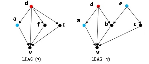
Figure 1: A simple example of Inf-CLDAG algorithm (red node $d$ is the positive seed and blue nodes $a$ and $e$ are negative seeds).

As an example, we show the computation for the structure of ${\it LDAG}^{+}(v)$ and ${\it LDAG}^{-}(v)$ of Figure 1. In the example, $d$ is the only positive seed while $a$ and $e$ are two negative seeds. In initialization, ${\it ap}^{+}(d,0)$, ${\it ap}^{-}(a,0)$ and ${\it ap}^{-}(e,0)$ are set to $1$ and all other values are set to $0$. In the first iteration, we start from the negative seeds $a$ and $e$ to do one level BFS traversal in ${\it LDAG}^{-}(v)$, and thus compute $P^{-}(b,1)$,$P^{-}(c,1)$, $P^{-}(v,1)$, ${\it ap}^{-}(b,1)$,${\it ap}^{-}(c,1)$ and ${\it ap}^{-}(v,1)$. Next we go to ${\it LDAG}^{+}(v)$ and do one level BFS traversal starting from the positive seed $d$, and compute ${\it ap}^{+}(f,1)$,${\it ap}^{+}(c,1)$ and ${\it ap}^{+}(v,1)$, which use the values $P^{-}(c,1)$ and $P^{-}(v,1)$ computed. Then we start the second iteration, which is second level BFS traversal in ${\it LDAG}^{-}(v)$, and this only gives us node $v$, for which we compute ${\it ap}^{-}(v,2)$. We will do another BFS traversal on ${\it LDAG}^{+}(v)$, and then we find that the BFS traversal has reached all nodes in both LDAGs and the computation finishes.

5.2 CLDAG algorithm.

Once we have the computation of negative influence reduction for any seed set as given in Algorithm 3, we can plug it into the greedy algorithm for positive seed selection. We call this algorithm CLDAG. We will present the complete pseudocode description of CLDAG algorithm here as Algorithm  4.

Algorithm 4 CLDAG($G,k,N_{0},\theta$)

1:  $S=\emptyset$

2:  //Build local structure

3:  for all node $v\ \in\ V$ do

4:     Build ${\it LDAG}^{+}(v),{\it LDAG}^{-}(v),OutLS^{+}(v)$ with threshold $\theta$

5:  end for

6:  //initialize DecInf

7:  set $DecInf(v)=0$ for all node $v\in V$

8:  for all node $v\ \in\ V$ and $v\not\in N_{0}$ do

9:     for all node $u\in{\it LDAG}^{+}(v)$ do

10:        $before={\it ap}^{-}(v,\emptyset)$

11:        $after={\it ap}^{-}(v,\{u\})$

12:        $DecInf(u)\,\mathrm{+=}\ before-after$

13:     end for

14:  end for

15:  //Main Loop

16:  for $i=1$ to $k$ do

17:     $s=\arg\max_{v\in V\setminus(S\cup N_{0})}DecInf(v)$

18:     //update influence reduction

19:     for all node $v\in OutLS^{+}(s)$ do

20:        for all node $u\in{\it LDAG}^{+}(v)$ do

21:           //subtract previous incremental influence reduction

22:           $DecInf(u)\,\mathrm{-=}\ {\it ap}^{-}(v,S\cup\{u\})-{\it ap}^{-}(v,S)$

23:           //add up new incremental influence reduction

24:           $DecInf(u)\,\mathrm{+=}\ {\it ap}^{-}(v,S\cup\{u,s\})-{\it ap}^{-}(v,S\cup\{s\})$

25:        end for

26:     end for

27:     //add node $s$ as positive seed

28:     $S=S\cup\{s\}$

29:  end for

30:  return $S$

The algorithm contains an initialization part and an iteration part. In initialization(line 3-5), we construct ${\it LDAG}^{+}(v)$ and ${\it LDAG}^{-}(v)$ for all nodes $v$. We also maintain an auxiliary set $OutLS^{+}(v)$, which is the set of nodes to which $v$ may have positive influence, i.e., $u\in OutLS^{+}(v)$ if and only if $v\in{\it LDAG}^{+}(u)$. Since positive seed set is changing in the algorithm, we use ${\it ap}^{-}(v,S)$ to represent the negative activation probability of $v$ in its LDAGs under positive seed set $S$. Then, for each node $u\in{\it LDAG}^{+}(v)$, we compute the incremental influence reduction ${\it ap}^{-}(v,\emptyset)-{\it ap}^{-}(v,\{u\})$ when adding $u\in{\it LDAG}^{+}(v)$ as a positive seed, and sum them up for each $u$ to get $DecInf(u)$, the overall incremental influence reduction of node $u$.

In the main iteration(line 16-29), we iterate $k$ times to select $k$ seeds. In each iteration, we select a new seed $s$ with the largest $DecInf(s)$. Once $s$ is selected, other nodes’ $DecInf(u)$ may need to be updated. Since $s$ may positively influence all nodes in $OutLS^{+}(s)$, thus all nodes $u\in{\it LDAG}^{+}(v)$ with $v\in OutLS^{+}(s)$ needs to update their $DecInf(u)$. Note that here we take advantage of the local DAG structure, so that we do not need to update the incremental influence reduction of every node in the graph. The update is done by using Algorithm 3.

Complexity Analysis. Let $n=|V|$, $m_{i\theta}^{+}=\max_{v}|{\it LDAG}^{+}(v)|$, $m_{i\theta}^{-}=\max_{v}|{\it LDAG}^{-}(v)|$, and $n_{o\theta}^{+}=\max_{v}|OutLS^{+}(v)|$. Let $t_{i\theta}^{+}$ and $t_{i\theta}^{-}$ be the time of efficient construction of ${\it LDAG}^{+}(v)$’s and ${\it LDAG}^{-}(v)$’s, respectively. Note that $m_{i\theta}^{+}=O(t_{i\theta}^{+})$ and $m_{i\theta}^{-}=O(t_{i\theta}^{-})$, and for sparse graphs, efficient Dijkstra shortest path algorithm implementation could make $t_{i\theta}^{+}$ and $t_{i\theta}^{-}$ close to the order of $m_{i\theta}^{+}$ and $m_{i\theta}^{-}$. We first analyze the complexity of storing all LDAG structures.

In the initialization step, we need to compute ${\it LDAG}^{+}(v)$’s and ${\it LDAG}^{-}(v)$’s for all nodes, and thus it takes $O(n(t_{i\theta}^{+}+t_{i\theta}^{-}))$ time. We use a max-heap structure to store $DecInf(u)$’s, and it takes $O(n)$ time to initialize. The $DecInf(u)$ computation by Algorithm 3 takes $O(n(m_{i\theta}^{+}+m_{i\theta}^{-}))$ time. Overall, initialization takes $O(n(t_{i\theta}^{+}+t_{i\theta}^{-}))$ time.

For the iteration step, each iteration needs to update $DecInf(u)$’s for at most $n_{o\theta}^{+}m_{i\theta}^{+}$ nodes, and each update involves influence computation by Algorithm 3, which takes $O(m_{i\theta}^{+}+m_{i\theta}^{-})$ time, plus updating $DecInf(u)$ on the max-heap, which takes $O(\log n)$ time. Therefore, the iteration step takes $O(kn_{o\theta}^{+}m_{i\theta}^{+}(m_{i\theta}^{+}+m_{i\theta}^{-}+\log n))$ time.

Hence the total time complexity of the algorithm is $O(n(t_{i\theta}^{+}+t_{i\theta}^{-})+kn_{o\theta}^{+}m_{i\theta}^{+}(m_{i\theta}^{+}+m_{i\theta}^{-}+\log n))$.

For space complexity, we store all LDAGs and $OutLS^{+}(v)$’s, so the space complexity is $O(n(m_{i\theta}^{+}+m_{i\theta}^{-}+n_{o\theta}^{+}))$. In actual implementations one may not afford to store all the LDAG structures (as in our implementation), so an alternative is to store only $OutLS^{+}(v)$’s and compute LDAGs whenever needed. It is easy to see that in this case, the time complexity is $O(n(t_{i\theta}^{+}+t_{i\theta}^{-})+kn_{o\theta}^{+}m_{i\theta}^{+}(t_{i\theta}^{+}+t_{i\theta}^{-}+\log n))$, which is not significantly worse than storing LDAGs, while the space complexity is reduced to $O(nn_{o\theta}^{+})$.

6 Experiments

To test the efficiency and effectiveness of CLDAG for influence blocking maximization problem under the CLT model, we conduct experiments on three real-world datasets as well as synthetic networks.

6.1 Experiment setting

The three real-world datasets are mobile network and collaboration networks. The mobile network is a graph derived from a partial call detailed record (CDR) data of a Chinese city from China Mobile, the largest mobile communication service provider in China. In the mobile network, every node corresponds to a mobile phone user and the edges correspond to their phone calls between one another. We use the number of calls between two users as the edge weight and normalize it among all edges incident to a node (the edge thus becomes directed with asymmetric edge weights). The NetHEPT and NetPHY are both collaboration networks extracted from the e-print arXiv (http://www.arXiv.org). The former is extracted from the ”High Energy Physics - Theory” section (form 1991 to 2003), and the latter is extracted from ”Physics” section, and both are the same datasets used in [6]. The nodes in both networks are authors and an edge between two nodes means the two authors coauthored at least one paper. We use the number of coauthored papers as the edge weight and normalize it among all edges incident to a node. Some basic statistics of these networks are shown in Table 1.

The edge weights described above do not differentiate between positive and negative weights yet. To differentiate them and study the effect of different diffusion strength for positive and negative diffusions, we introduce positive propagation rate $p^{+}$ and negative propagation rate $p^{-}$, both of which are values from $0$ to $1$. We multiply edge weight with $p^{+}$ and $p^{-}$ of each edge to obtain its positive and negative edge weight, respectively. The effect is that all positive edge weights of in-edges of a node sums up to $p^{+}$, and thus with probability $1-p^{+}$ the node will not be activated even if all of its in-neighbors are positively activated. The case for $p^{-}$ is similar.

Table 1: Statistics of the three real-world networks.

Dataset	Mobile	NetHEPT	NetPHY
Node	15.5K	15.2K	37.1K
Edge	37.0K	58.9K	231.5K
Average Degree	4.77	7.75	12.48

We compare the performance of the following algorithm and heuristics:

• CLDAG: Our CLDAG algorithm with $\theta=0.01$;

• Greedy: Algorithm 1 under the CLT model with the lazy-forward optimization of [18], and 10000 simulation runs for each influence estimate.

• Degree: a baseline heuristic, simply choosing nodes with largest degrees as positive seeds.

• Random: a baseline heuristic, simply choosing nodes at random as positive seeds.

• Proximity Heuristic: A simple heuristic under which we choose the direct out-neighbors of negative seeds as positive seeds to block the negative influence. Among these direct out-neighbors, we sort them by the negative weights of their in-edges connecting them with negative seeds, and select the top $k$ nodes as the positive seeds.

Proximity heuristic introduced above is based on the simple idea of trying to block the influence of negative seeds at their direct neighbors. It should be noticed that the proximity heuristic can be considered as a simplified version of our CLDAG algorithm. In fact, for each node $v$, if we construct its ${\it LDAG}^{+}(v)$ to be only the node $v$ itself, while its ${\it LDAG}^{-}(v)$ to be $v$ itself if $v$ has no in-neighbors in the negative seed set $N_{0}$, or else to be $v$ with one of $v$’s in-neighbors in $N_{0}$ with the largest negative edge weight to $v$. It is easy to verify that our CLDAG algorithm under these LDAG structures exactly matches the proximity heuristic. Therefore, proximity heuristic can be treated as an intermediate algorithm between the baseline random algorithm and the full-blown CLDAG algorithm, and is helpful for understanding the features of CLDAG.

Since the CLT model is a probabilistic model, when we evaluate the blocking effect for any given positive and negative seed sets, we test it for 1000 times and take their average as the result. The negative seeds in $N_{0}$ are chosen either randomly or from nodes with the largest degrees. The scalability test is run on Intel Xeon E5504 2G*2 (4 cores for every CPU), 36G memory server, while all others are run on Dell D630 laptop with 2G memory. All experiment code is written in C++.

6.2 Results with the greedy algorithm.

We first run tests that include the greedy algorithm. Since the greedy algorithm runs very slow on large graphs, we extract two subgraphs from the datasets for comparison. One subgraph is a 1000 node graph extracted from the mobile network, and another is a 5000 node graph extracted from the NetHEPT network. The extraction is done by randomly selecting a node in the graph and doing BFS from the node until we obtain the desired number of nodes, and we include all edges for these nodes in the subgraph. We choose 50 nodes with the highest degrees as negative seeds and select 200 positive seeds to block their influence. Both $p^{+}$ and $p^{-}$ are set to 1. The experiment result are showed in Figure 2.

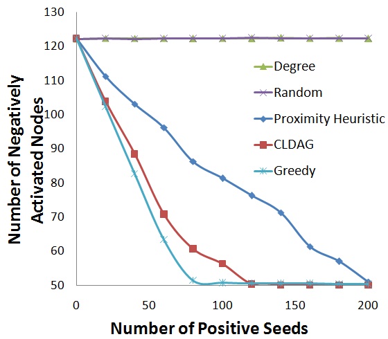
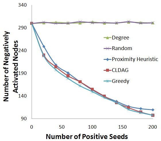
(a)Mobile	(b)NetHEPT
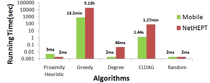
(c)Running time for selecting 200 seeds

Figure 2: Experiment result of comparison with Greedy algorithm.

From Figure 2 (a) and (b), we can see that the CLDAG algorithm consistently matches the performance of the greedy algorithm for both datasets. In the 1000-node mobile network test, CLDAG significantly outperforms the Proximity heuristic, e.g., when CLDAG completely blocks all negative influence with 130 seeds, proximity heuristic still allows negative influence to reach about 30 more nodes. In term of negative influence reduction, this is $(120-50)/(120-80)=175\%$ improvement. In the 5000-node NetHEPT dataset, proximity heuristic performs as well as CLDAG and the greedy algorithm. In both cases, random and degree heuristic perform badly, essentially having no blocking effect at all. This is in contrast with degree heuristic result for influence maximization reported in the previous papers [6, 5, 7], where degree heuristic still have moderate gain when selecting more seeds. Our interpretation is that for influence blocking maximization, knowing where the negative seeds are becomes very important, and thus proximity heuristic could behave reasonably well while degree heuristic oblivious to the location of negative seeds becomes useless.

From Figure 2 (c), we see that CLDAG is much faster than the greedy algorithm, with more than two orders of magnitude speedup. With 5000 nodes, the greedy algorithm already takes more than five hours, while CLDAG only takes one minute to select 200 seeds.

We further compare the scalability of CLDAG with the greedy algorithm. For this test, we use a family of synthetic power-law graphs generated by the DIGG package [9]. We generate graphs with doubling number of nodes, from 0.2K, 0.4K, up to 6.4K, using power-law exponent of 2.16. Each size has 10 different random graphs and our running time result is the average among the runs on these 10 graphs. We randomly choose 50 nodes as negative seeds and find 50 positive seeds to block the negative influence. We set both $p^{+}$ and $p^{-}$ to 1. The scalability result is shown in Figure 3.

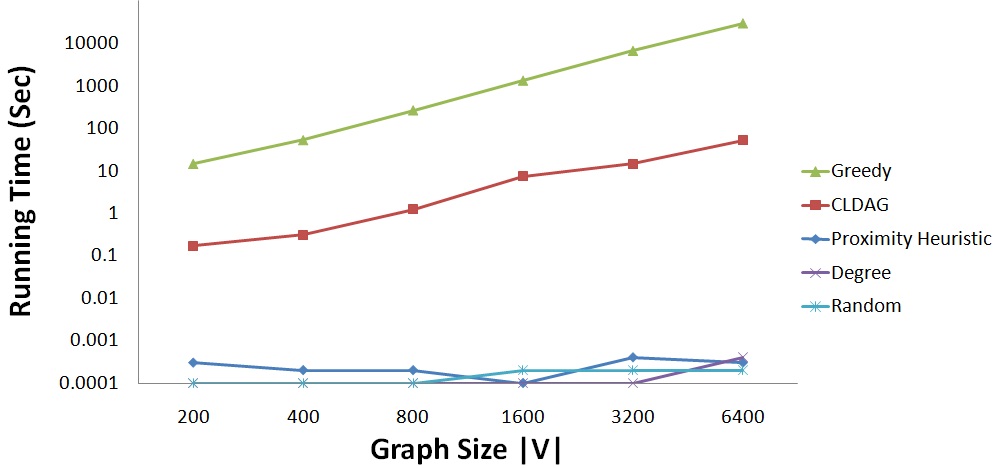
Figure 3: Experiment result on algorithm scalability.

The result clearly shows that CLDAG is two orders of magnitude faster than the greedy algorithm and its running time has linear relationship with the size of the graph, which indicates good scalability of the CLDAG algorithm. Therefore, comparing with the greedy algorithm, CLDAG matches the blocking effect of the greedy algorithm while has at least two orders of magnitude speedup in running time.

6.3 Results on larger dataset without the greedy algorithm.

We conduct experiments on the full graphs of the three datasets, but we do not include the greedy algorithm since its running time becomes too slow. The initial negative seeds are chosen either randomly or with highest degrees. We first set $p^{+}$ and $p^{-}$ to 1.

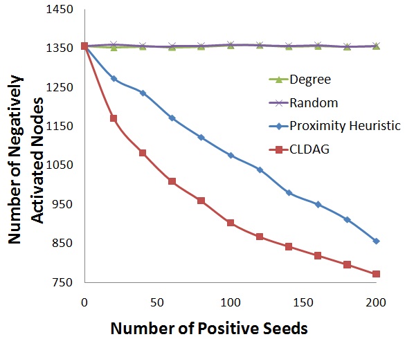
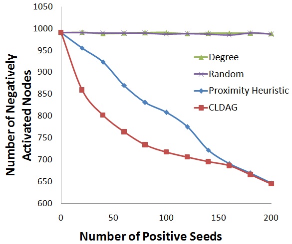
(a)NetHEPT: Max degree	(b) NetHEPT:Random
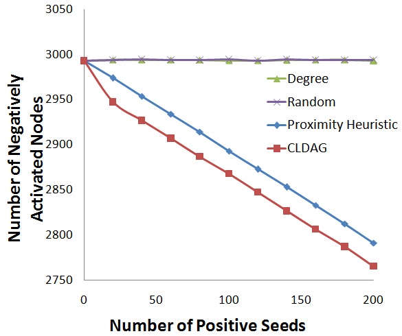
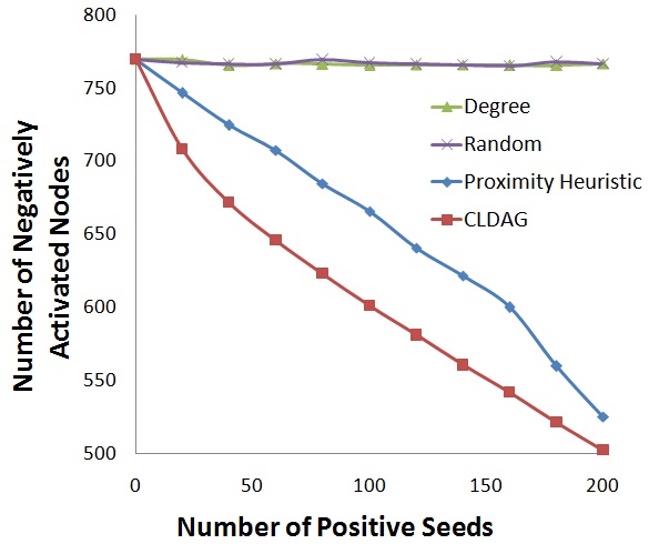
(c)Mobile: Max degree	(d) Mobile:Random
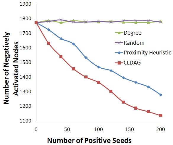
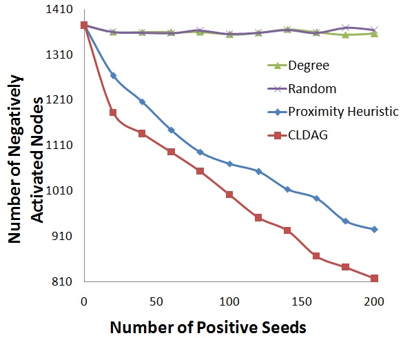
(e)NetPHY: Max degree	(f) NetPHY:Random
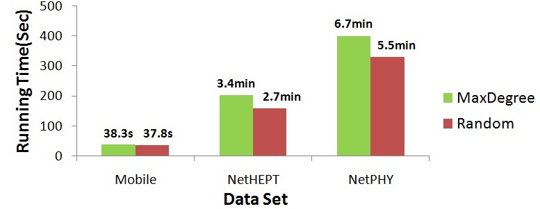
(g) Running Time of CLDAG algorithm on real networks

Figure 4: Experiment result of CLT model on three real dataset. We choose 200 negative seeds with max degree in experiment (a),(c),(e) and 400 random negative seeds in experiment (b),(d),(f).

As shown in Figure 4 (a) to (f), the performance of CLDAG strictly dominates the proximity heuristic in all cases. For random negative seed selection, the negative influence reduction of CLDAG is on average 78.24% higher than that of the proximity algorithm (percentage taken as the average of results from $1$ seed to $200$ seeds). For max-degree negative seed selection, CLDAG improves the performance of proximity heuristic even more, for 80.75% on average. Degree and random heuristic still show no blocking effect on all test cases. The running time of CLDAG is consistently low, as shown in Figure 4 (g). The results demonstrate that across all networks and all negative seed selection methods, CLDAG has consistently good performance in negative influence reduction over other heuristics, and it achieves this good performance efficiently.

Next, we vary propagation rate $p^{+}$ and $p^{-}$ to check their effect on influence dissemination and the performance of our algorithm. For simplicity, we only present experiment result on the NetHEPT network. We choose 200 nodes with max degree as negative seeds and select 200 positive nodes to block their influence. In one test we have $p^{+}=0.5$ and $p^{-}=1$, and thus negative influence diffusion is stronger, while in the second test, we use $p^{+}=1$ and $p^{-}=0.5$, making positive influence diffusion stronger.

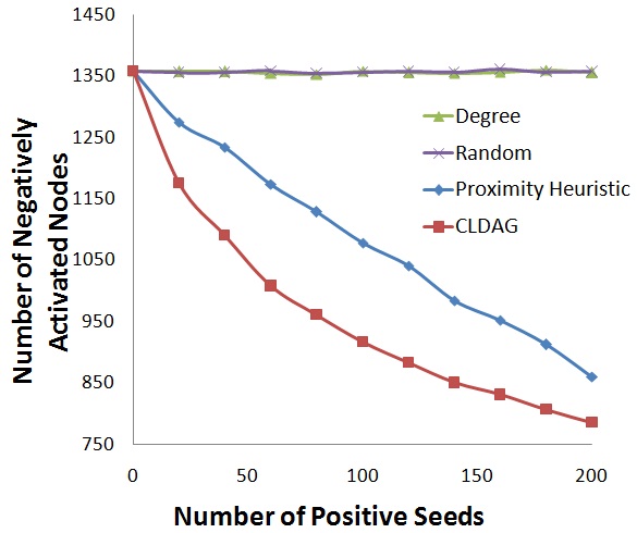
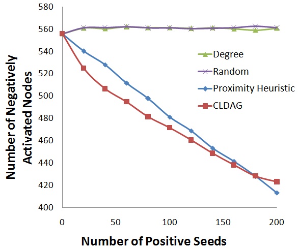
(a) $p^{+}=0.5$, $p^{-}=1$	(b) $p^{+}=1$, $p^{-}=0.5$

Figure 5: Experiment result of CLT model on propagation rate $p^{+}$ and $p^{-}$.

Figure 5 reports our simulation results. First, as expected, when the negative influence is stronger, more nodes become negative without positive influence ($1350$ nodes vs. $560$ nodes in our two test cases). More importantly, we see that our CLDAG algorithm performs much better than the proximity heuristic when the negative influence is stronger (Figure 5 (a)). This is because in this case negative diffusion can traverse long paths and thus simply placing positive seeds next to the negative seeds may not block the negative diffusion well. On the other hand, when the negative influence is weak (Figure 5 (b)), negative influence could be effectively blocked by placing positive seeds next to them, and thus proximity heuristic performs close to CLDAG.

To summarize, our results show that CLDAG has the best performance among tested heuristics across all graphs, and especially when negative influence diffusion is strong. Proximity heuristic as a simplified version of CLDAG has reasonable performance in a few cases especially when negative influence diffusion is weak, and can be used as a fast alternative to CLDAG in this case. However, there are situations in which proximity heuristic is significantly worse than CLDAG. Traditional degree heuristic cannot be used for influence blocking maximization at all from our test results.

6.4 Effectiveness of influence blocking at different negative seed size.

Finally, we test the effectiveness of influence blocking with CLDAG, when the size of negative seeds increases. We vary the negative seed size from $1$ to $1000$, and see how many positive seeds are required by CLDAG to reduce negative influence to $10\%$. We cap the number of positive seeds at $1000$. For this test, we use the NetHEPT network, select negative seeds with largest degrees, and set $p^{+}=p^{-}=1$. The results are shown in Table 2, where $\sigma_{N}(S,N_{0})$ denotes the expected number of negative activations with positive seeds $S$ and negative seeds $N_{0}$.

Table 2: Result on the effectiveness of influence blocking

$|N_{0}|$	$\sigma_{N}(\emptyset,N_{0})$	$|S|$	$\sigma_{N}(S,N_{0})$
1	72.8979	23	6.7396
2	77.4516	68	6.0182
5	156.48	145	15.6667
10	213.077	199	20.6628
20	581.366	557	57.6617
50	963.633	926	95.8451
100	1006.37	1000	108.823
200	1669.85	1000	680.518
500	3635.95	1000	2640.8
1000	5836.48	1000	4845.58

The result shows that it requires about $20$ to $30$ times of positive seeds to reduce negative influence to about $10\%$ level, and it becomes increasingly hard to block negative influence. For example, with $1000$ negative seeds, we spend an equal number of $1000$ positive seeds but can only reduce $17\%$ negative influence. Therefore, first mover has a clear advantage, and the best way to block negative influence is before it becomes pervasive.

7 Conclusion and Discussions

In this work, we study influence blocking maximization problem under the competitive linear threshold model. We show that the objective function of the IBM problem is submodular under the CLT model, and thus the greedy approximation algorithm is available. We then design an efficient algorithm CLDAG to overcome the slowness of the greedy algorithm. Our simulation results demonstrate that CLDAG matches the greedy algorithm in the blocking effect while significantly improving running time. CLDAG also outperforms other heuristic algorithms such as proximity heuristic that selects direct neighbors of negative seeds, showing that CLDAG is a stable and robust algorithm for the IBM problem.

Finally, we compare two closely related results in the literature, which showing some interesting subtleties in competitive influence diffusion. First, in [3], Budak et al. study the IBM problem for the extended IC model. They show, however, that when we extend the IC model to allow positive and negative diffusions having two set of different parameters, the IBM is not submodular. This indicates a subtle difference between different diffusion models. In this sense, CLT model is more expressive, since it is easier to model different diffusion strength in the CLT model and see its effect, as we did in our evaluation (Figure 5). They also show that when restricting the positive weights to be $1$, or to be the same as negative weights, the problem becomes submodular. For these cases, we are able to design efficient algorithms close to MIA and MIA-N of [5, 4], and our simulations results are similar when comparing with the greedy algorithm and other heuristics, but we do not report them here.

Second, in [2], Borodin et al. propose several competitive diffusion models extended from the LT model. In particular, their separate threshold model is essentially the CLT model in this paper (with a slightly different tie-breaking rule). Interestingly, they show that the problem of maximizing positive influence given a fixed negative seed set is not submodular (applicable to our CLT model), while we show here that influence blocking maximization is submodular. Intuitively, this is because even though a positive seed $x$ blocks the negative influence, to maximize positive influence it may also need other positive seeds to activate nodes that are blocked from negative influence by node $x$. Therefore, the marginal gain of $x$ is larger for the positive influence maximization objective when there are other positive seeds corporating with $x$, making it not submodular.

Several improvements and future directions are possible. One direction is looking into even faster and more space-efficient algorithms for influence blocking maximization. Another direction is to tackle the IBM problem in other competitive diffusion models, especially models without submodularity property.

Appendix

A Proof of Theorem 4.1

• Consider an instance of the NP-complete vertex cover problem defined by an undirected $|V|$-node graph $G=(V,E)$ and an integer $k$. The vertex cover problem asks if there exists a set $S$ of $k$ nodes in $G$ so that every edge has at least one endpoint in $S$. We show that this can be reduced to the IBM problem under the CLT model.

Given an instance of the vertex cover problem involving a graph $G$, let $d_{G}(v)$ denote the degree of node $v$ in $G$ and define $d_{m}=\max_{v\in V}d_{G}(v)$. We construct a corresponding instance of the IBM problem as follows. We first construct a directed graph $G^{\prime}$ from $G$. Besides the original graph structure, for each vertex $v_{i}$ in $G$, we build a spindle structure $S_{i}$ with $|V|+2$ nodes and a chain $C_{i}$ with $\ell+1$ nodes, and $S_{i}$ and $C_{i}$ share the node $v_{i}$. We use a toy example given in Figure 6 to describe our construction.

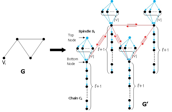
Figure 6: Graph construction for the NP-hardness proof (positive edges are red, and negative seeds and negative edges are blue).

As shown in the Figure 6, each spindle structure consists of a top node, $|V|$ intermediate nodes and a bottom node. The top node is chosen as a negative seed and has $|V|$ negative edges (meaning positive weight is $0$) with negative weight $1$ to each of the intermediate nodes. Each intermediate node has a negative edge with $\frac{1}{|V|}$ negative weight to the bottom node. Then we use each bottom node of all spindle structures to form a similar graph as $G$ except that we direct all edges of the origin $G$ in both directions to build positive edges (meaning negative weights are $0$). The positive weights of positive edges are set according to the degree of the according node in $G$. Namely for the bottom node $v_{i}$ of spindle structure $S_{i}$, we set all the weights of positive in-edges of $v_{i}$ equally to $\frac{1}{d_{G}(v_{i})}$. Next, starting from $v_{i}$, we add a chain with $\ell+1$ nodes (including $v_{i}$) and $\ell$ directed negative edges of weight $1$. We set $\ell=\lceil\frac{|V|d_{m}}{|V|-1}-1\rceil$. Thus the total size of constructed graph $G^{\prime}$ is $O(|V|^{2})$.

We first show Lemma A.1 for our NP-hardness proof.

Lemma A.1

In the constructed graph $G^{\prime}$, given positive seed set $S$ if there exists a bottom node $v$ in a spindle structure whose positive activation probability at step $1$ is not strictly $1$, a higher negative influence reduction with one more positive seed can be achieved by choosing $v$ instead of selecting any other intermediate node in spindle structure or any node in chains.

• We assume that the positive activation probability for node $v$ at step $1$ is $p^{+}$. Firstly, it is obvious that choosing bottom node is a better strategy than choosing node in any chain. Then by adding node $v$ to the positive seed set, we can have a negative influence reduction $\Delta_{v}\geq(1-p^{+})(\ell+1)$. By adding any intermediate node to positive seed set, we can have $\Delta_{inter}\leq 1+\frac{1}{|V|}(1-p^{+})(\ell+1)$. With $\ell=\lceil\frac{|V|d_{m}}{|V|-1}-1\rceil$, we can easily get $\Delta_{v}\geq(1-p^{+})(\ell+1)>1+\frac{1}{|V|}(1-p^{+})(\ell+1)\geq\Delta_{inter}$. Therefore choosing bottom node $v$ will always lead to greater gain in negative influence reduction than any other intermediate or chain nodes. $\Box$

If there is a vertex cover $S$ of size $k$ in $G$, then one can deterministically make $\sigma_{{\it NIR}}(S)=|V|(\ell+1)$ by choosing the positive seed set as the vertex cover of graph $G$. Since without the positive seeds all nodes in $G^{\prime}$ will be negatively activated, while with positive seed set $S$ we can save the bottom nodes and also the nodes on the chains. Conversely this is the only way to get a set with $\sigma_{{\it NIR}}(S)\geq|V|(\ell+1)$. Otherwise if positive seeds among bottom nodes are not a vertex cover of the origin graph $G$, the probability that all bottom nodes can be positively activated in step $1$ is strictly less than $1$, and the gap is at least $1/d_{m}$. According to Lemma A.1, all $k$ positive seeds must be chosen among the bottom nodes. Thus, in step $2$ any node that was not positive in step $1$ must become negative, due to negative influence dominance. Hence, we have $\sigma_{{\it NIR}}(S)\leq(|V|-1)(\ell+1)+(1-\frac{1}{d_{m}})(\ell+1)<|V|(\ell+1)$. Therefore, by checking if $G^{\prime}$ has a positive seed set of size $k$ that achieves negative influence reduction of at least $|V|(\ell+1)$, we can know if the original graph $G$ has a vertex cover of size $k$. $\Box$

References

- [1] S. Bharathi, D. Kempe, and M. Salek. Competitive influence maximization in social networks. In WINE, pages 306–311, 2007.
- [2] A. Borodin, Y. Filmus, and J. Oren. Threshold models for competitive influence in social networks. In WINE, pages 539–550, 2010.
- [3] C. Budak, D. Agrawal, and A. E. Abbadi. Limiting the spread of misinformation in social networks. In WWW, pages 665–674, 2011.
- [4] W. Chen, A. Collins, R. Cummings, T. Ke, Z. Liu, D. Rincón, X. Sun, Y. Wang, W. Wei, and Y. Yuan. Influence maximization in social networks when negative opinions may emerge and propagate. In SDM, pages 379–390, 2011.
- [5] W. Chen, C. Wang, and Y. Wang. Scalable influence maximization for prevalent viral marketing in large-scale social networks. In KDD, pages 1029–1038, 2010.
- [6] W. Chen, Y. Wang, and S. Yang. Efficient influence maximization in social networks. In KDD, pages 199–208, 2009.
- [7] W. Chen, Y. Yuan, and L. Zhang. Scalable influence maximization in social networks under the linear threshold model. In ICDM, pages 88–97, 2010.
- [8] P. Clifford and A. Sudbury. A model for spatial conflict. Biometrika, 60(3):581–688, 1973.
- [9] L. Cowen, A. Brady, and P. Schmid. DIGG: DynamIc Graph Generator. http://digg.cs.tufts.edu.
- [10] J. Goldenberg, B. Libai, and E. Muller. Using complex systems analysis to advance marketing theory development: Modeling heterogeneity effects on new product growth through stochastic cellular automata. Academy of Marketing Science Review, 2001(9):1–18, 2001.
- [11] M. Granovetter. Threshold Models of Collective Behavior. American Journal of Sociology, 83(6):1420, 1978.
- [12] X. He, G. Song, W. Chen, and Q. Jiang. Influence blocking maximization in social networks under the competitive linear threshold model. arXiv technical report, to appear.
- [13] R. A. Holley and T. M. Liggett. Ergodic theorems for weakly interacting infinite systems and the voter model. Annals of Probability, 3:643–663, 1975.
- [14] D. Kempe, J. M. Kleinberg, and E. Tardos. Maximizing the spread of influence through a social network. In KDD, pages 137–146, 2003.
- [15] D. Kempe, J. M. Kleinberg, and E. Tardos. Influential nodes in a diffusion model for social networks. In ICALP, pages 1127–1138, 2005.
- [16] M. Kimura and K. Saito. Tractable models for information diffusion in social networks. In PKDD, pages 259–271, 2006.
- [17] J. Kostka, Y. A. Oswald, and R. Wattenhofer. Word of mouth: Rumor dissemination in social networks. In SIROCCO, pages 185–196, 2008.
- [18] J. Leskovec, A. Krause, C. Guestrin, C. Faloutsos, J. M. VanBriesen, and N. S. Glance. Cost-effective outbreak detection in networks. In KDD, pages 420–429, 2007.
- [19] R. Narayanam and Y. Narahari. Determining the top-k nodes in social networks using the shapley value. In AAMAS, pages 1509–1512, 2008.
- [20] G. Nemhauser, L. Wolsey, and M. Fisher. An analysis of the approximations for maximizing submodular set functions. Mathematical Programming, 14:265–294, 1978.
- [21] N. Pathak, A. Banerjee, and J. Srivastava. A generalized linear threshold model for multiple cascades. In ICDM, pages 965–970, 2010.
- [22] M. Richardson and P. Domingos. Mining knowledge-sharing sites for viral marketing. In KDD, pages 61–70, 2002.
- [23] T. C. Schelling. Micromotives and Macrobehavior. W. W. Norton & Company, 1978.
- [24] D. Trpevski, W. K. S. Tang, and L. Kocarev. Model for rumor spreading over networks. Physics Review E, 81:056102, May 2010.
- [25] Y. Wang, G. Cong, G. Song, and K. Xie. Community-based greedy algorithm for mining top-k influential nodes in mobile social networks. In KDD, pages 1039–1048, 2010.