Thermal decomposition of a honeycomb-network sheet – A Molecular Dynamics simulation study

Abstract

The thermal degradation of a graphene-like two-dimensional honeycomb membrane with bonds undergoing temperature-induced scission is studied by means of Molecular Dynamics simulation using Langevin thermostat. We demonstrate that at lower temperature the probability distribution of breaking bonds is highly peaked at the rim of the membrane sheet whereas at higher temperature bonds break at random everywhere in the hexagonal flake. The mean breakage time $\tau$ is found to decrease with the total number of network nodes $N$ by a power law $\tau\propto N^{-0.5}$ and reveals an Arrhenian dependence on temperature $T$. Scission times are themselves exponentially distributed. The fragmentation kinetics of the average number of clusters can be described by first-order chemical reactions between network nodes $n_{i}$ of different coordination. The distribution of fragments sizes evolves with time elapsed from initially a $\delta$-function through a bimodal one into a single-peaked again at late times. Our simulation results are complemented by a set of $1^{st}$-order kinetic differential equations for $n_{i}$ which can be solved exactly and compared to data derived from the computer experiment, providing deeper insight into the thermolysis mechanism.

I Introduction

Thermal degradation and stabilization of polymer systems has been a long-standing focus of research from both practical and fundamental viewpoints Allen . Plastic waste disposal has grown rapidly to ecological menace prompting researchers to investigate plastic recycling by degradation as an alternative Madras . On the other hand, degradation of polymers and other high molecular weight materials in different environments is usually a major limiting factor in their application. Thermal degradation (or, thermolysis) plays a decisive role in the design of flame-resistant polyethylene and other plastic materials Nyden . Another interesting aspects for applications include reversible polymer networks Sijbesma1 ; Sijbesma2 , and most notably, graphene, as a ”material of the future” that shows unusual thermomechanical properties Peeters ; Aluru . Recently, with the rapidly growing perspective of exploiting bio-polymers as functional materials Schulten ; Han , the stability of such materials has become an issue of primary concern Lindahl ; Sinha as, e.g., that of double-stranded polymer decomposition Metanomski .

Most theoretical investigations of polymer degradation have focused on determining the rate of change of average molecular weight Jellinek ; Ballauff ; Ziff ; Cheng ; Nyden2 ; Doerr ; Wang ; Hathorn ; Doruker ; Flegg . The main assumptions of the theory are that each link in a long chain molecule has equal strength and equal accessibility, that they are broken at random, and that the probability of rupture is proportional to the number of links present. Therefore, all of the afore-mentioned studies investigate exclusively the way in which the distribution of bond rupture probability along the polymer backbone affects the fragmentation kinetics and the distribution of fragment sizes as time elapses. In a recent study Paturej ; PaturejEPL , using Molecular Dynamics (MD) simulation with a Langevin thermostat, we observed a rather complex interplay between the polymer chain dynamics and the resulting bond rupture probability. A major role in this was attributed to the one-dimensional (1D) topological connectivity of the linear polymer. Significant change in rupture kinetics is observed while polymer architecture is tuned as in the case of thermolysis of adsorbed bottle-brushes bb1 ; bb2 .

Understanding the interplay between elastic and fracture properties is even more challenging and important in the case of 2D polymerized networks (elastic-brittle sheets). A prominent example of biological microstructure is spectrin, the red blood cell membrane skeleton, which reinforces the cytoplasmic face of the membrane. In erythrocytes, the membrane skeleton enables it to undergo large extensional deformations while maintaining the structural integrity of the membrane. A number of studies, based on continuum- Skalak , percolation- Srolovitz ; Saxton ; Seifert , or molecular level Monette ; Dao considerations of the mechanical breakdown of this network, modeled as a triangular lattice of spectrin tetramers, have been reported so far. Another example concerns the thermal stability of isolated graphene nanoflakes. It has been investigated recently by Barnard and Snook Snook using ab initio quantum mechanical techniques whereby it was noted that the problems “has been overlooked by most computational and theoretical studies”. Many of these studies can be viewed in a broader context as part of the problem of thermal decomposition of gels Argyropoulos , epoxy resins Rico ; Zhang and other 3D networks, studied both experimentally Argyropoulos ; Rico ; Zhang , and by means of simulations Kober as in the case of Poly-dimethylsiloxane (PDMS). In most of these cases, however, mainly a stability analysis is carried out whereas still little is known regarding the collective mechanism of degradation, the dependence of rupture time on system size, as well as the decomposition kinetics, especially as far as (2D) polymer network sheets are concerned. It is also interesting from the standpoint of basic physics to compare the degradation process to the one taking place in linear polymers where considerable progress has been achieved recently Paturej . Therefore, in the present work we extend our investigations to the case of (2D) polymer network sheets, embedded in 3D-space, and study as a generic example the thermal degradation of a suspended membrane with honeycomb orientation.

The paper is organized as follows: after a brief introduction, we sketch our model in Sec. II. In Sec. III we present our simulation results, that is, the distribution of bond scission rates over the membrane surface, the Mean First Breakage Time (MFBT) of a bond depending on membrane size and temperature, the distribution of recombination events - Sec. III.1, and the temporal evolution of the fragmentation process - Sec. III.2. We also develop a theoretical scheme based on a set of $1^{st}-$order kinetic differential equations, describing the time variation of the number of network nodes, connected by a particular number of bonds to neighboring nodes - Sec. III.3. We demonstrate that the analytical solution of such system provides a faithful description of the fragmentation kinetics. In Sec. IV we conclude with a brief discussion of our main findings.

II METHODS

II.1 Model

We study a coarse-grained model of honeycomb membrane embedded in three-dimensional (3D) space. In this investigation we consider generally symmetric hexagonal membranes (flakes) (Fig. 1). In a very few cases we also discuss fracture of a ribbon shape membranes. The membrane flake consists of $N$ spherical particles (beads, monomers) of diameter $\sigma$ connected in a honeycomb lattice structure whereby each monomer is bonded with three nearest-neighbors except of the monomers on the membrane edges which have only two bonds (see Fig. 1 [upper panel]). The total number of monomers $N$ in such a membrane is $N=6L^{2}$ where by $L$ we denote the number of monomers (or hexagon cells) on the edge of the membrane (i.e., $L$ characterizes the linear size of the membrane). There are altogether $N_{bonds}=(3N-6L)/2$ bonds in the membrane.

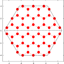
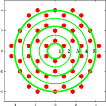
Figure 1: [upper panel] A model of a membrane with honeycomb structure that contains a total of $N=54$ beads and has linear size $L=3$ ($L$ is the number of beads or hexagonal cells on the edge of the membrane). [lower panel] An example of subdivision of beads and bonds, composing a membrane with $L=3$, into subgroups (“circles”). The total number of circles $C$ in the membrane of linear size $L$ is $C=2L-1$.

We find it appropriate to divide the two-dimensional membrane network so that all the beads and bonds are distributed into different subgroups presented by concentric “circles” with consecutive numbers (see Fig. 1 [upper panel]) proportional to the radial distance from the membrane center. To odd circle numbers thus belong beads and bonds that are nearly tangential to the circle. Even circles contain no beads and only radially oriented bonds (shown to cross the circle in Fig. 1. The total number of circles $C$ in the membrane of linear size $L$ is found to be $C=(2L-1)$. We use this example of dividing the beads and the bonds composing the membrane in order to represent our simulation results in appropriate way which relates them to their relative proximity to membrane’s periphery.

II.2 Potentials

The nearest-neighbors in the membrane are connected to each other by ”breakable bonds” described by a Morse potential, where $r$ is a distance between the monomers,

$$U_{\text{M}}(r)=\epsilon_{M}\{1-\exp[-\alpha(r-r_{\text{min}})]\}^{2}$$ (1)

$\alpha=1$ is a constant that determines bond elasticity and $r_{\text{min}}=1$ is the equilibrium bond length. The dissociation energy of a given bond is $\epsilon_{M}=1$, measured in units of $k_{B}T$, where $k_{B}$ denotes the Boltzmann constant and $T$ is the temperature. The minimum of this potential occurs at $r=r_{\text{min}},\;~{}U_{\text{Morse}}(r_{\text{min}})=0$. The maximal restoring force of the Morse potential, $f_{\text{max}}=-dU_{\text{M}}/dr=\alpha\epsilon_{M}/2$, is reached at the inflection point, $r_{\mbox{\tiny inflex}}=r_{\text{min}}+\alpha^{-1}\ln(2)\approx 2.69$. This force $f_{\text{max}}$ determines the maximal tensile strength of the membrane. Stretching of the bond beyond $r_{\mbox{\tiny inflex}}$ means potentially a scission of that bond as far as the restoring force declines rapidly with bond length even though there is a chance for a recombination. Therefore we take as a criterion for breaking a bond its expansion to $r_{h}=5$ beyond which practically a bond recombinantion is ruled out. Since $U_{\text{M}}(0)\approx 2.95$, the Morse potential, Eq. (1), is only weakly repulsive and beads could partially penetrate one another at $r<r_{\text{min}}$. Therefore, in order to allow properly for the excluded volume interactions between bonded monomers, we take the bond potential as a sum of $U_{\text{M}}(r)$ and the so called Weeks-Chandler-Anderson (WCA) potential, $U_{\text{WCA}}(r)$, (i.e., the shifted and truncated repulsive branch of the Lennard-Jones potential),

$$U_{\text{WCA}}(r)=\begin{cases}4\epsilon\left[\left(\frac{\sigma}{r}\right)^{12}-\left(\frac{\sigma}{r}\right)^{6}\right]+\epsilon,&\text{for}~{}~{}r\leq 2^{1/6}\sigma\\ 0,&\text{for}~{}~{}r>2^{1/6}\sigma\end{cases}$$ (2)

with parameter $\epsilon=1$ and monomer diameter $\sigma=2^{-1/6}\approx 0.89$ so that the minimum of the WCA potential coincides with the minimum of the Morse potential. Thus, the length scale is set by the parameter $r_{\text{min}}=2^{1/6}\sigma=1$. The nonbonded interactions between monomers are taken into account by means of the WCA potential, Eq. (2). The nonbonded interactions in our model correspond to good solvent conditions whereas the bonded interactions make the bonds in our model breakable so they undergo scission at sufficiently high $T$.

We have been anxious to emphasize the common features of failure in materials with similar architecture but largely varying elasticity properties, e.g., from $1000$ GPa graphene’s Young modulus Aluru compared to $4\times 10^{-3}$ GPa for spectrin Dao . Putting the value of a Kuhn segment to $\sigma=1.44$ Å and taking the thermal energy $k_{B}T=4\times 10^{-21}$ J at $T=300$ K, we get from our simulation graphene_force a Young modulus $0.03$ GPa which is ranged between typical values for rubber-like materials $0.01$–$0.1$ GPa.

II.3 MD algorithm

In our MD simulation we use Langevin dynamics, which describes the Brownian motion of a set of interacting particles whereby the action of the solvent is split into slowly evolving viscous (frictional) force and a rapidly fluctuating stochastic (random) force. The Langevin equation of motion is the following:

$$m\overrightarrow{\dot{v}_{i}}(t)=\overrightarrow{F}_{i}(t)-m\gamma\overrightarrow{v_{i}}(t)+\overrightarrow{R}_{i}(t)$$ (3)

where $m$ denotes the mass of the particles which is set to $m=1$, $\overrightarrow{v}_{i}$ is the velocity of particle $i$, $\overrightarrow{F}_{i}=(\overrightarrow{F}_{\textmd{M}}+\overrightarrow{F}_{\textmd{WCA}})_{i}$ is the conservative force which is a sum of all forces exerted on particle $i$ by other particles in the system, $\gamma$ is the friction coefficient and $\overrightarrow{R}_{i}$ is the three dimensional vector of random force acting on particle $i$. The random force $\overrightarrow{R}_{i}$, which represents the incessant collision of the monomers with the solvent molecules, satisfies the fluctuation-dissipation theorem $\langle R_{i\alpha}(t)R_{j\beta}(t^{\prime})\rangle=2\gamma k_{B}T\delta_{ij}\delta_{\alpha\beta}\delta(t-t^{\prime})$ where the symbol $\langle\ldots\rangle$ denotes an equilibrium average and the greek-letter subscripts refer to the $x$, $y$ or $z$ components. The friction coefficient $\gamma$ of the Langevin thermostat is generally set to $\gamma=0.25$ and only in very few cases to $10$. The integration step is $0.002$ time units (t.u.) and the time is measured in units of $r_{\text{min}}\sqrt{m/\epsilon_{M}}$. We emphasize at this point that in our coarse-grained modeling no explicit solvent particles are included. In this work the velocity-Verlet algorithm is used to integrate the equations of motion.

Our MD simulations are carried out in the following order. First, we prepare an equilibrated membrane conformation, starting with a fully flat configuration shown schematically in Fig. 1, where each bead in the network is separated by a distance $r_{\text{min}}=1$ equal to the equilibrium separation of the bond potential $(U_{\text{M}}+U_{\text{WCA}})$ [see Eq. (1), and Eq. (2)]. Then we start the simulation with this prepared conformation and let the membrane equilibrate in the heat bath for a very long period of time ($\approx 10^{7}$ integration steps) at a temperature low enough that the membrane stays intact, Fig. 2, (this equilibration is done in order to prepare different starting conformations for each simulation). Then the temperature is raised to the working temperature and the membrane is equilibrated for 20 MD t.u. ($10^{4}$ integration steps) which interval was found as sufficient to establish equipartition (uniform distribution of the temperature throughout the membrane).

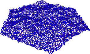
Figure 2: A snapshot of a typical conformation of an intact membrane with $L=30$ containing $5400$ monomers after equilibration. Characteristic ripples are seen to cross the surface.

The time then is set to zero and we continue the simulation of this membrane conformation to examine the thermal scission of the bonds. We measure the elapsed time $\tau$ until the first bond rupture occurs and repeat the above procedure for a large number of events ($10^{3}$–$10^{4}$) so as to sample the stochastic nature of rupture and to determine the mean $\langle\tau\rangle$ which we refer to as the Mean First Breakage Time. In the course of simulation we also calculate properties such as the probability distribution of breaking bonds regarding their position in the membrane (a rupture probability histogram), the probability distribution of the first breakage time $W(\tau)$, the mean extension of the bonds with respect to the consecutive circle number in the membrane, as well as other quantities of interest.

Since in the problem of thermal degradation there is no external force acting on the membrane edges, a well-defined activation barrier for a bond scission is actually missing, in contrast to the case of applied tensile force. Therefore, a definition of an unambiguous criterion for bond breakage is not self-evident. Moreover, depending on the degree of stretching, bonds may break and then recombine again. Therefore, in our numeric experiments we use a sufficiently large value for critical extension of the bonds, $r_{h}=5r_{\text{min}}$, which is defined as a threshold to a broken state of the bond. This convention is based on our checks that the probability for recombination (self-healing) of bonds, stretched beyond $r_{h}$, is sufficiently small, $<10^{-5}$ .

Also we examine the course of the degradation kinetics: at periodic intervals in separate simulations runs we analyze the size distribution of fragments (clusters) of the initial membrane and establish the time-dependent probability distribution function of fragment sizes, $P(n,t)$, as time elapses after the onset of the thermal degradation process. This also yields the time evolution of the mean fragment size, $N(t)=\int_{0}^{\infty}n(t)P(n,t)dn$. We perform the statistical averaging of fragment sizes by developing an appropriate for the system fast cluster counting algorithm.

The Molecular Dynamics calculations were carried out using a cluster counting algorithm based on an ad hoc implementation of the Hoshen-Kopelman program Hoshen_Kopelman . In a subsequent paper of Al-Futaisi and Patzek Patzek , the Hoshen-Kopelman algorithm for cluster labeling has been extended to non-lattice environments where network elements (sites or bonds) are placed at random points in space. Following Al-Futaisi and Patzek Patzek , we developed our simplified version of this algorithm which concerns only clusters of nodes in a network with honeycomb structure (which is our model shown in Fig. 2). In our implementation we assume that all nodes in the network are occupied, but some links can be broken when we study thermal degradation process of the network. The network information is stored in two arrays. The first one is related to the connectivity of the nodes and the second to the state of links (intact or broken link)

III RESULTS and DISCUSSION

III.1 Bond scission

.

.

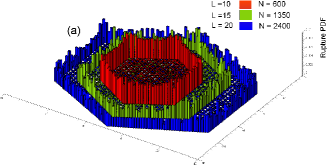
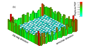
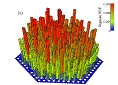
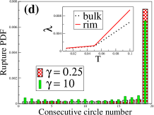
Figure 3: (a) Rupture probability histograms for thermally induced scission events in flexible honeycomb flake of different linear size $L$ as shown in the legend. (b) Rupture histogram for a ribbon-like square honeycomb membrane with $496$ nodes. (c) Rupture histogram for a membrane flake with beads tethered at the rim, $L=10$. Parameters of the heat bath are $T=0.1$ and $\gamma=0.25$. (d) Probability distribution of breakage events as a function of consecutive circle number for a membrane flake with $N=600$ and two different friction coefficients $\gamma=0.25$ and $10.0$. Here $T=0.1$. The inset shows estimated values of Lyapunov exponents $\lambda$ vs $T$ for beads located in the rim/bulk of membrane as indicate. Here $N=5400$, $\gamma=0.25$.

In Fig. 3a we show the distribution of bond scission rates among all bonds of the honeycomb membrane for flakes (with zig-zag pattern on the periphery) of several sizes $L=10,\;15,\;20$. Somewhat surprisingly, one finds the overwhelming fraction of bond breaking occurs at the outer-most rim of the membrane where monomers are bound by only two bonds to the rest of the sheet. We have also sampled the rupture histograms for ribbon-like square membranes, Fig. 3b. Interestingly, we observe no difference between the rupture rates of zig-zag and armchair edges whereas the bonds in the four corners of such membrane expectedly break more frequently. The difference in the relative stability of the bonds becomes clearly evident in Fig. 3d where the frequency of periphery bonds appears nearly two orders of magnitude larger when compared to bonds in the ’bulk’ of the membrane where each monomer (node) is connected by three bonds to its neighbors. One may therefore conclude that a moderate increase in the coordination number of the nodes (by only 33% regarding the maximum coordination of a node) leads to a major stabilization of the supporting bonds and much stronger resistance to fracture. Our additional simulation in the strongly damped regime for $\gamma=10$ indicates no qualitative changes compared to $\gamma=0.25$ except an absolute overall increase of the rupture times which is natural for a more viscous environment.

Note that the question of where and which bonds predominantly break is by no means trivial. For example, in the case of linear polymer chain thermal decomposition the rate of bond rupture is least at both chain ends although the end monomers, in contrast to those inside the chain, are bound by a single bond only Paturej . We demonstrate in Fig. 3c that this interesting feature holds also for the honeycomb membrane flake, provided the rim is clamped and left immobile during the simulation. Evidently, the highest frequency of bond scissions grows towards the membrane center. Similar to the case of polymer chains with fixed ends Paturej ; Lee .

In order to provide deeper insight into the mechanism of temperature-induced bond breaking, in the inset to Fig. 3d we present the temperature variation of Lyapunov’s exponent $\lambda$ for membrane nodes located in the bulk and in the rim of the sheet. Evidently, beyond a cross-over temperature $T\approx 0.05$ one observes a significant growth of $\lambda_{\mbox{\tiny rim}}$ as compared to $\lambda_{\mbox{\tiny bulk}}$. This indicates that the trajectories of nodes at the membrane periphery attain much faster chaotic features at higher temperature than those of the bulk nodes. Moreover, we should note that beads in the vortices have values of $\lambda$ which exceed those in the rim by about $5\%$. Therefore this analysis of trajectory stability at characteristic locations in the membrane clearly demonstrate that bond rupture is induced by intermittent motion of the respective nodes.

The variation of the MFBT $\tau$ of a bond with membrane size $N$ during thermolysis for both hexagonal and square shapes of the 2D sheet is displayed in Fig. 4a. Evidently, one observes for $\tau$ a well pronounced power law behavior, $\tau\propto N^{-\beta}$ with an exponent $\beta\approx 0.50\pm 0.03$. It turns out that the scaling exponent $\beta$ remains insensitive to changes in the geometric shape of the membrane sheet. This value of $\beta$ might appear somewhat surprisingly to deviate from the expected exponent of unity, given that in the absence of external force all bonds are supposed to break completely at random so that the total probability for a bond scission (i.e., the chance that any bond might break within a time interval) is additive and should be, therefore, proportional to the total number of available bonds, $N_{bonds}=(3N-6L)/2$. As suggested by Fig. 3, however, predominantly only periphery bonds are found to undergo scission during thermal degradation. The number of periphery bonds goes roughly as $\propto\sqrt{N}$ which agrees well with the observed value $\beta\approx 0.5$ and provides a plausible interpretation of the simulation result, Fig. 4a. From the inset in Fig. 4a one may verify that the bond scission displays an Arrhenian dependence on inverse temperature, $\tau\propto\exp(\Delta E_{b}/k_{B}T)$, with a slope $\Delta E_{b}\approx 1$. This slope suggests a dissociation energy $\Delta E_{b}$ of the order of the potential well depth of the Morse interaction, Eq. (1) where $\epsilon_{M}=1.0$. In our model we deal typically with $E_{b}/(k_{B}T)\approx 10$ which at $300$ K and typical bond length $r_{\mbox{\tiny min}}\approx 0.144$ nm, corresponds to ultimate tensile stress $\sim 0.6$ GPa. This is a reasonable value for our membrane which is considerably softer than graphene with $\sim 100$ GPa Aluru and is ranged between typical values for rubber materials $~{}0.01$–$0.1$ GPa.

The probability distribution function (PDF) of MFBT $W(t)$, i.e., the PDF of the time interval before the first breakage event in the membrane takes place, is shown in Fig. 4b for $T=0.1$. Evidently, one has $W(t)\propto\exp(-t/\tau)$ with a sharp maximum close to $t\approx 0$. At even lower temperature one might expect this maximum to become more pronounced, suggesting

.

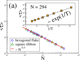
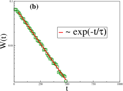
Figure 4: (a) Mean first breakage time $\langle\tau\rangle$ vs. number of beads $N$ for two different membrane shapes: a hexagonal flake and a square ribbon. Solid line represents a fit by power law with an exponent $\beta=0.5$ in both cases. The inset shows the variation of $\langle\tau\rangle$ with inverse temperature $1/T$ for a flake membrane with $N=294$ particles. The fitting line yields an Arrhenian relationship, $\langle\tau\rangle\propto\exp(\Delta E_{b}/k_{B}T)$ with dissociation energy barrier $\Delta E_{b}\approx 0.95$. (b) Breakage time probability distributions $W(t)$ for thermally induced breakage of a flake membrane with $N=600$ particles at $T=0.1$. Symbols denote result of the simulation and full line stands for a fitting function $W(t)\propto\exp(-t/\tau)$ with $\tau=128.2$.

thus a Poisson distribution for the $W(t)$. As far as $\tau$ tends to grow exponentially fast with decreasing $T$ - see inset in Fig. 4a, collecting statistics in this temperature range becomes difficult.

We also analyze the fracture of bonds with respect to their possible recombination. The procedure of sampling bond recombination events is the following. Once one of the bonds in the membrane is stretched to the position of the Morse potential inflexion point $r_{\mbox{\tiny inflex}}\approx 2.69$ (corresponding to maximal tensile strength of a given bond), we start to monitor its further expansion for $10^{4}$ integration steps and record its maximal expansion $h=r-r_{\mbox{\tiny inflex}}$. If the bond subsequently shrinks to $r<r_{\mbox{\tiny inflex}}$, this is counted as recombination event. Simultaneously we record the time $t$ needed to go back below the expansion $r_{\mbox{\tiny inflex}}$. We then compute distributions $Q_{h}(h)$ of bond expansions beyond $r_{\mbox{\tiny inflex}}$ and recombination times $P_{h}(t)$. Thus $Q_{h}(h)$ yields the probability of bond overstretching to distance $h=r-r_{\mbox{\tiny inflex}}$ during the recombination event. As indicated by the distribution $P_{h}(t)$ shown in Fig. 5, the interval $20$ t.u. exceeds more than five times the maximal life of recombination which guarantees that all such events are properly taken into account. Generally we find that a recombination of bonds takes place rather seldom (roughly once per simulation run of average length 130 t.u., as given by the MFBT).

It has been mentioned in Sec. II that in the absence of external force acting on the membrane the criterion for a bond to be considered broken is not unambiguous. Adopting a rather large critical bond extension of $r_{h}=5r_{\mbox{\tiny min}}$ practically rules out the probability of of subsequent recombination of such bonds, as indicated by $Q_{h}(h)\propto\exp(-3.2h)$ in 5 (right inset).

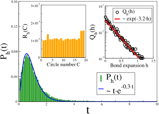
Figure 5: Probability distribution $P_{h}(t)$ of times (impulses), and $Q_{h}(h)$ of bond overstretching lengths $h$ (circles, right panel of inset) before a recombination event in a membrane with $N=600$, $T=0.1$, $\gamma=0.25$ takes places. The recombination times probability distribution $P_{h}(t)$ is fitted by Poisson distribution (blue line). The probability for a bond stretching a distance $h$ beyond $r_{\mbox{\tiny inflex}}$ is described by $Q_{h}(h)$ indicating an exponential decay - red line. The left inset shows healing probability $R_{h}$ vs. consecutive circle number, demonstrating which part of the membrane undergoes healing most frequently.

Indeed, if one adopts $r_{\mbox{\tiny inflex}}$ as a threshold for rupture than $Q_{h}(h)$ suggests that bond expansions larger than $r_{\mbox{\tiny inflex}}+1.1\approx 3.79$ practically never happen. The PDF $P(t)$ of times elapsed before self-healing is also shown in Fig. 5 where it appears as a Poisson distribution, $P(t)\approx t\exp(-0.3t)$. Not surprisingly, most of the recombination occur in the periphery of the membrane - left inset in Fig. 5.

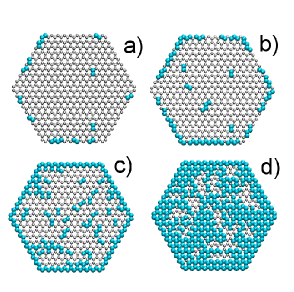
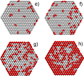
Figure 6: Thermal breakage of bonds in a membrane made of $N=600$ particles at different time moments: a) $t=10^{2}$, b) $7\cdot 10^{2}$ c) $5\cdot 10^{4}$ d) $3\cdot 10^{5}$ and e) $50$, f) $100$, g) $250$, h) $500$. Broken bonds are marked by blue ($T=0.1$) or red ($T=0.15$) color, depending on the temperature of a heat bath, while gray color corresponds to intact bonds.

In Fig. 6 we show the distribution of broken bonds at different times after the onset of thermal degradation. We would like to note that the regular hexagonal flakes shown in Fig. 6 serve only to indicate schematically the positions of both broken and still intact bonds and by no means represent the actual conformation of the membrane. Two different temperatures, $T=0.10$ and $T=0.15$ are studied. One can readily verify from Fig. 6a-d that at $T=0.10$ the degradation process starts from the rim of the network sheet and then proceeds inwards, as noted earlier by Meakin Meakin . In contrast, at $50\%$ higher temperature, i.e., at $T=0.15$, bonds break everywhere in the network sheet - cf. Fig. 6b, f and Fig. 6c, g. Such difference in the bond scission mechanism at different temperatures has been observed Meakin before. It appears that at $T=0.1$ the membrane periphery undergoes stronger oscillations than the membrane bulk which lead to bond scission at the rim while in the inner part of the sheet the monomers mutually block each other and the bonds remain largely intact. This explanation is supported by the measured values of Lyapunov exponents (see the inset of Fig. 3 and discussion in Sec. III A). On the other hand a ’hot’ i.e. at $T=0.15$ membrane undergoes much stronger agitation as a whole and as a result bonds break all over the network sheet. Moreover, at lower $T$ when the thermal agitation of the membrane is weaker, one may correlate the probability of bond scission with the average strain in the bonds -

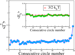
Figure 7: Variation of mean squared bond length $\langle l^{2}\rangle$ vs. distance from membrane center (consecutive circle number) for thermolysis of membrane composed of $N=5400$ beads. The inset displays mean kinetic energy $\langle E_{k}\rangle$ (per monomer) as a function of circle number. Red dashed line represents the level of energy which corresponds to equipartition theorem. Parameters of thermostat are $T=0.1$ and $\gamma=0.25$.

Fig. 7. Evidently, the average squared bond length $\langle l^{2}\rangle$ increases steadily and becomes nearly $8\%$ larger for the bonds sitting on the last ring of the membrane whereas no difference in the mean kinetic energy between peripheral and bulk nodes is detected - Fig. 7. Note that the kinetic energy (that is, the temperature $T$) is thereby uniformly distributed along the sheet - see inset in Fig. 7.

III.2 Temporal evolution of the fragmentation process

After the onset of the thermal decomposition process the membrane flake disintegrates into smaller clusters (fragments) of size $n$ whose mean size (or average molecular weight) $N(t)$ decreases steadily with time. $N(t)$ is easily accessible experimentally, therefore we give in Fig. 8a the course of its temporal evolution, observed in our computer experiment. Using an ad hoc cluster counting program in the course of the MD-simulation we sample the

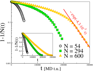
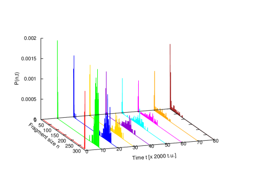
Figure 8: (a) Semi-log plot of time variation of mean fragment size $N(t)$ for membranes made of different size as indicated. Symbols represent simulation results whereas a red line stands for the fitting function $1-1/N(t)\propto\exp{(-kt)}$. The kinetic constant $k=4.3^{-5}s^{-1}$. In the inset the same is shown in normal coordinates. (b) Probability distribution of fragment sizes $P(n,t)$ at different times $t$ (in MD time units) after beginning of the thermal degradation process for a membrane with $N=294$. Parameters of a heat bath are $T=0.12$ and $\gamma=0.25$.

probability distribution of fragment sizes, $P(n,t)$, so that the first moment $N(t)=\int n(t)P(n,t)dn$ gives the cluster mean size $N(t)$. Thus, for a given time moment $t$ we average data over more than $10^{3}$ independent runs, each starting from a different initial conformation of the honeycomb membrane. In Fig. 8b we show the time variation of the ensuing PDF $P(n,t)$ whereby the system is seen to start with a single sharp peak at $t=0$ when the membrane is still intact. As time goes by, $P(n,t)$ becomes bimodal, the maximum of the distribution is seen to shift to smaller values of cluster size whereas an accumulation of fragments of size $1$ or $2$ is observed to contribute to a second peak at $n\approx 1$. Eventually, as $t\rightarrow\infty$, the PDF $P(n,t)$ settles to a shape with a single sharp peak (a $\delta$-function) at $n\approx 1$ (not shown here).

One can readily see from Fig. 8a that the quantity $1-N^{-1}(t)$ does not immediately follow a straight line of decay when plotted in semi-logarithmic coordinates, rather, such a decay is observed after an initial period of slower decline. This effect is due to averaging over many realizations of the fragmentation process. In each run the degradation of bonds starts earlier or later at a particular time $\tau$ (the Mean First Breakage Time) that is distributed according to $W(\tau)$ - cf. Fig. 4b. As a result a clear cut exponential course of $1-N^{-1}(t)$ is only observed in the late stages of fragmentation. Such behavior is found independently of the membrane size - Fig. 8a.

In addition, one could expect that the fragmentation process is not governed by a single rate constant in a presumably $1^{st}-$order chemical reaction even though the bonds that undergo rupture are chemically identical. Therefore, from the temporal mean cluster size behavior, presented in Fig. 8a, one may conclude that even in the case of a homogeneous membrane the thermal degradation process is more adequately described by several reaction constants which govern the dissociation of different groups of bonds. In the next section we suggest a simple model of reaction kinetics which takes into account this conjecture.

III.3 Reaction kinetics

One may try to reproduce the bond scission kinetics during in the course of thermal fragmentation by a set of several $1^{st}$-order chemical reactions. The nodes of the membrane can be subdivided into several groups, depending on the number of intact bonds that connect them to neighboring nodes. In the case of a honeycomb membrane one may distinguish four such groups, and denote the instantaneous number of such nodes (monomers) by $n_{0},\;n_{1},\;n_{2}$ and $n_{3}$ whenever $0,\;1,\;2,$ or $3$ intact bonds exist around such a node. If self-recombination of bonds is ignored, which is reasonable in view of large value of the threshold, and simultaneous scission of two and more bonds is disregarded as hardly probable, one can write down a strongly simplified set of $1^{st}$-order kinetic differential equations (DE) that describes the evolution of $n_{0}(t),\;n_{1}(t),\;n_{2}(t)$ and $n_{3}(t)$ with time:

$$\dot{n}_{1}(t) = -k_{1}n_{1}(t)+k_{2}n_{2}(t)$$ (4)

$$\dot{n}_{2}(t) = -k_{2}n_{2}(t)+k_{3}n_{3}(t)$$

$$\dot{n}_{3}(t) = -k_{3}n_{3}(t)$$

Thus, for example, the number of double-bonded nodes decreases as one of the two bonds breaks, however, if a bond breaks around a node with triple coordination this would increase the population of double-bonded nodes. Note, that the total number of nodes of all kinds remains thereby conserved,

$$n_{0}(t)+n_{1}(t)+n_{2}(t)+n_{3}(t)=N=6L^{2}.$$ (5)

If the degradation process starts with an intact membrane conformation at $t=0$ (no broken bonds exist), one can fix the initial conditions as $n_{0}(0)=0,\;n_{1}(0)=0,n_{2}(0)=6L$ and $n_{3}(0)=N-n_{2}(0)=6L(L-1)$. Thus, initially one has only $n_{2}(0)=6L$ double-bonded nodes at the membrane periphery along with $n_{3}(0)=6L(L-1)$ triple-bonded nodes in the bulk of the flake. Then, as the decomposition process develops, nodes from a given class $r=1,\;2,\;3$ will transform into a lower class $r=0,\;1,\;2$ ones (we neglect hereby the simultaneous scission of more than one bond of a node as highly improbable event). Eventually, at $t\rightarrow\infty$ the fragmentation process ends and one expects $n_{1}(\infty)=n_{2}(\infty)=n_{3}(\infty)=0$ and $n_{0}(\infty)=N$.

One may solve analytically the system of $1^{st}$-order DE Eqs. (4) to a set of functions $n_{i}(t)$ with $0\leq i\leq 3$:

$$n_{0}(t) = 6L^{2}-n_{1}(t)-n_{2}(t)-n_{3}(t)$$

$$n_{1}(t) = \frac{6L}{(k_{1}-k_{2})(k_{1}-k_{3})(k_{2}-k_{3})}\left[k_{1}(k_{2}-k_{3})\left(e^{-k_{3}t}-e^{-k_{1}t}\right)+k_{2}k_{3}\left(e^{-k_{3}t}-e^{-k_{2}t}\right)\right.$$

$$+ \left.k_{1}k_{3}L\left(e^{-k_{3}t}-e^{-k_{2}t}\right)-k_{2}k_{3}L\left(e^{-k_{3}t}-e^{-k_{1}t}\right)+k_{3}^{2}L\left(e^{-k_{2}t}-e^{-k_{1}t}\right)\right]$$

$$n_{2}(t) = 6L\frac{\left(k_{2}e^{-k_{2}t}-k_{3}e^{-k_{3}t}-k_{3}Le^{-k_{2}t}+k_{3}Le^{-k_{3}t}\right)}{k_{2}-k_{3}}$$ (7)

$$n_{3}(t) = 6L(L-1)e^{-k_{3}t}$$

where the rate constants $k_{1},\;k_{2}$ and $k_{3}$ are still to be determined, for example, by comparison with simulation data. As one may readily verify from Fig. 3, our simulation data suggest that a bond to a triple-bonded node at $T=0.12$ is much more stable (by about two orders of magnitude) than a bond at the flake periphery where each node is connected by only two bonds to the network. Thus the system of Eqs. (6) can be tested for a set of reaction constants $k_{1}\gg k_{2}>k_{3}$ directly by means of our Molecular Dynamics computer experiment.

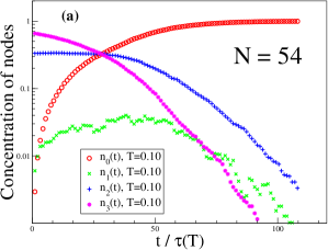
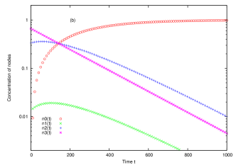
Figure 9: (a) Variation of the number of nodes $n_{m}(t)$ with $m=0$–$3$ intact bonds with elapsed dimensionless time $t/\tau(T)$ for a membrane with $N=54$ and $T=0.10$. Here $\tau(T)$ denotes the characteristic time of degradation at the respective temperature $T$. The $n_{1}(t)$ (monomers bound by a single bond) are shown by shaded area. (b) The same as in (a) for the same membrane size $N=54$ according to the analytic result Eqs. (6). The values of the kinetics rate constants are $k_{1}=20.0,\;k_{2}=0.007,\;k_{3}=0.005$.

Indeed, one finds by comparing the simulation result, Fig. 9a for a membrane of size $N=54$ at $T=0.10$, and the analytical solution, Eqs. (6), Fig. 9b, that the observed kinetics agree qualitatively, provided one allows for the absence of fluctuation in Eqs. (4) (i.e., for the disarray and averaging of the MFBT $\tau$ in the simulation data). We should like to point out here that the values of the rate constants $k_{1},\;k_{2},\;k_{3}$ are not best fit values. Because of the additional effect of averaging discussed in Sec. III.2 and shown in Fig. 8, a straight fitting procedure with three parameters $k_{1},k_{2},k_{3}$ would be both inefficient and hardly successful. Therefore we tried different combinations of values for $k_{1},k_{2},k_{3}$ subject to the condition that $k_{1}\gg k_{2}>k_{3}$. Even though the general qualitative shapes turn out to be rather sensitive to the values of $k_{1},k_{2},k_{3}$ (being capable of reproducing, e.g., the existence of a common intersection point of $n_{0}(t),n_{2}(t)$ and $n_{3}(t)$ - see Fig. 9a - for particular choice of parameters), one finds thus easily a combination which qualitatively matches well the simulation data shown in Fig. 9a.

One may conclude therefore that the simplified set of $1^{st}-$order DE Eqs. (4) captures qualitatively the main features of the fragmentation kinetics and the principal mechanism at work is a combination of few $1^{st}-$order chemical reactions of bond scission. Nonetheless, it is conceivable to expect that for a full quantitative description of the thermal degradation process the set of kinetic equations, Eqs. (4), should be extended by few additional reactions: $n_{1}(t)\rightarrow n_{2}(t),\;n_{2}(t)\rightarrow n_{3}(t)$ that may in principle also take place (with respective rate constants). One can then still derive an analytical solution of the extended set of DE that describes the full kinetics of fragmentation and try to fit the ensuing rate constants to the simulation data. In view of the growing number of fit parameters, however, a detailed analysis of such system is beyond the scope of the present work and should be left for future work.

IV CONCLUSION

In the present investigation we use Langevin Molecular Dynamics simulation and also solve a set of $1^{st}-$order kinetic DE so as to model the process of thermal destruction of a polymerized membrane sheet with honeycomb structure. Results of our work can be treated as generally applicable due to the fact that a two-dimensional regular lattice can only be created in few ways: honeycomb, triangular and square lattice with second neighbor interactions because of the zero-shear modulus (apart from exotic cases like quasi-crystalline, kagome, etc. lattices of little relevance). The differences in lattice coordination among the first three periodic networks induce only quantitative renormalization of the Young modulus. However they don’t change the overall elastic behavior. Our findings regarding the most salient features of thermolysis in an elastic brittle honeycomb network sheet subject to sufficiently high temperature can be summarized as follows:

• The probability of bond scission is highest at the periphery of the membrane sheet where nodes are connected by two bonds only. At higher temperature, however, the whole sheet undergoes fragmentation whereby also bonds in the bulk rupture.

• The mean time $\tau$ until a bond undergoes scission event declines with the number of nodes $N$ (with membrane size) by a power law as $\tau\propto N^{-0.5}$ independently of the geometric shape of membrane sheet. The times of bond scission are exponentially distributed, $W(t)\propto\exp(-t/\langle\tau\rangle)$.

• Bond recombination (self-healing) occurs seldom during thermal degradation, and the measured recombination times follow Poisson distribution whereas an extra-stretching of bonds (beyond the point of maximal tensile strength) before a recombination takes place is exponentially improbable.

• the fragmentation kinetics is determined by $1^{st}$-order reactions between network nodes with different number of intact bonds and follows simple exponential decay at late times.

• A set of $1^{st}$-order kinetic differential equations, describing the process of fragmentation, can be established and solved analytically. One finds results in qualitative agreement with those from computer experiment providing thereby a deeper insight into the mechanism of thermal degradation of two-dimensional honeycomb networks.

In view of the presented results, it should be clear that more work is needed (e.g., regarding the effects of randomness in brittle networks) until a full understanding of the process of thermal degradation in polymerized $2D$-membranes is reached.

V Acknowledgments

J.P. would like to thank the Institute of Physical Chemistry at the Bulgarian Academy of Sciences for hospitality during his stay. A. M. gratefully acknowledges support by the Max-Planck-Institute for Polymer Research during the time of this investigation. This study has been supported by the Deutsche Forschungsgemeinschaft (DFG), Grant Nos. SFB625/B4 and FOR597. H.P. and A.M. acknowledge the use of computing facilities of Madara Computer Center at Bulg. Acad. Sci.

References

- (1) N.S Allen and M. Edge, Fundamentals of Polymer Degradation and Stabilization, Elsevier Applied Science, New York, 1966.
- (2) G. Madras, J.M. Smith and B.J. McCoy, Ind. Eng. Chem. Res. 35, 1795 (1996).
- (3) M.R. Nyden, G.P. Forney and G.E. Brown, Macromolecules 25, 1658 (1996).
- (4) R.P. Sijbesma, F.H. Beijer, L. Brunsveld, B.J.B. Folmer, J.H.K.K. Hirschberg, R.F. Lange, J.K.L. Lowe, and E.W. Meijer Science 278, 1601 (1997).
- (5) R.P. Sijbesma and E.W. Meijer, Chem. Commun. 1, 5 (2003).
- (6) M. Neek-Amal and F.M. Peeters, Phys. Rev. B 81, 235437 (2010); Phys. Rev. B 82, 085432 (2010); Appl. Phys. Lett. 97, 153118 (2010).
- (7) H. Zhao, K. Min and N.R. Aluru, Nano Letters, 9 (8) 3012 (2009); H. Zhao, and N.R. Aluru, Jour. Appl. Phys. 108, 064321 (2010); K. Min and N.R. Aluru N.R. Appl. Phys. Lett. 98, 013113 (2011).
- (8) M. Sarikaya, C. Tamerler, A.K.Jen, K.L. Schulten and F. Banyex, Nature Mater. 2, 577 (2003).
- (9) T.H. Han, J. Kim, J.S. Park, C.B. Park, H. Ihee and S.O. Kim, Adv. Mater. 19, 3924 (2007).
- (10) T. Lindahl, Nature (London) 362, 709 (1993).
- (11) R.P. Sinha and D.-P. Hader, Photochem. Photobiol. Sci. 1, 225 (2002).
- (12) W.V. Metanomski, R.E. Bareiss, J. Kahovec, K.L. Loening, L. Shi and V.P. Shibaev, Pure Appl. Chem. 65, 1561 (2002).
- (13) H.H.G. Jellinek, Trans. Faraday Soc. 1944, 266 (1944)
- (14) M. Ballauff and B. A. Wolf, Macromolecules, 14, 654 (1981).
- (15) R.M. Ziff and E.D. McGrady, Macromolecules 19, 2513 (1986); E.D. McGrady and R.M. Ziff, Phys. Rev. Lett. 58, 892 (1987).
- (16) Z. Cheng and S. Redner, Phys. Rev. Lett. 60, 2450 (1988).
- (17) E. Blaisten-Barojas and M. R. Nyden, Chem. Phys. Lett. 171, 499 (1990); M.R. Nyden and D.W. Noid, J. Phys. Chem. 95, 940 (1991).
- (18) T.P. Doerr and P.L. Taylor, J. Chem. Phys. 101, 10107 (1994).
- (19) M. Wang, J.M. Smith, and B.J. McCoy, AIChE Journal, 41, 1521 (1995).
- (20) B. C. Hathorn, B. G. Sumpter, and D. W. Noid, Macromol. Theory Simul. 10, 587 (2001).
- (21) P. Doruker, Y. Wang, and W. L. Mattice, Comp. Theor. Polym. Sci. 11, 155 (2001).
- (22) M.B. Flegg, P.K. Pollett and D.K. Gramotnev, Phys. Rev. E 77, 021105 (2007); Phys. Rev. E , 78, 031117 (2008).
- (23) J. Paturej, A. Milchev, V.G. Rostiashvili and T.A. Vilgis, J. Chem. Phys. 134, 224901 (2011).
- (24) J. Paturej, A. Milchev, V.G. Rostiashvili and T.A. Vilgis, EPL 94, 48003 (2011).
- (25) A. Milchev, J. Paturej, V.G. Rostiashvili, T.A. Vilgis, Macromolecules 44, 3981 (2011).
- (26) J. Paturej, L. Kuban, A. Milchev, T.A. Vilgis, EPL 97, 4371 (2012).
- (27) J.C. Hansen, R. Skalak, S. Chien and A. Hoger. Biophys. J. 70, 146 (1996).
- (28) P.D. Beale, and D.J. Srolovitz, Phys. Rev. E 37, 5500 (1988).
- (29) M.J. Saxton, Biophys. J. 57, 1167 (1990).
- (30) D.H. Boal, U. Seifert and A. Zilker Phys. Rev. Lett. 69, 3405 (1992).
- (31) L. Monette and M.P. Anderson, Modelling Simul. Mater. Sci. 2, 53 (1994).
- (32) M. Dao, J. Li and S. Suresh Mater. Sci. Eng. C, 26, 1232 (2006).
- (33) A.S. Barnard and I.K. Snook, J. Chem. Phys. 128, 094707 (2008).
- (34) D.S. Argyropoulos and H.I. Bolker, Macromolecules, 20, 2915 (1987); Macromol. Chem., 189, 607 (1988).
- (35) L. Barral, F.J. Diez, S. Garcia-Garabal, J. Lopez, B. Montero, R. Montes, C. Ramirez and M. Rico, Europ. Polym. J. 41, 1662 (2005).
- (36) Z. Zhang, G. Liang, P. Ren and J. Wang, J. Polym. Composites 28, 755 (2007).
- (37) K. Chenoweth, S. Cheung, A.C.T. van Duin, W.A. Goddard III, E.M. Kober, J. Am. Chem. Soc. 127, 7192 (2005).
- (38) J. Hoshen and R. Kopelman, R. Phys. Rev. B 14, 3438 (1976).
- (39) A. Al-Futaisi and T.W. Patzek, Physica A 321, 665 (2003).
- (40) C.F. Lee, Phys. Rev. E 80, 031134 (2009).
- (41) J. Paturej, H. Popova, A. Milchev, T.A. Vilgis Phys. Rev. E 85, 021805 (2012).
- (42) C.L. Dias, J. Kröger, D. Vernon and M. Grant, Phys. Rev. E 80, 066109 (2009).
- (43) P. Meakin and Z. Xu, Prog. Comp. Fluid Dyn. 9, 399 (2009) (doi: 10.1504/PCFD.2009.027371).