Measuring reproducibility of high-throughput experiments

Abstract

Reproducibility is essential to reliable scientific discovery in high-throughput experiments. In this work we propose a unified approach to measure the reproducibility of findings identified from replicate experiments and identify putative discoveries using reproducibility. Unlike the usual scalar measures of reproducibility, our approach creates a curve, which quantitatively assesses when the findings are no longer consistent across replicates. Our curve is fitted by a copula mixture model, from which we derive a quantitative reproducibility score, which we call the “irreproducible discovery rate” (IDR) analogous to the FDR. This score can be computed at each set of paired replicate ranks and permits the principled setting of thresholds both for assessing reproducibility and combining replicates.

Since our approach permits an arbitrary scale for each replicate, it provides useful descriptive measures in a wide variety of situations to be explored. We study the performance of the algorithm using simulations and give a heuristic analysis of its theoretical properties. We demonstrate the effectiveness of our method in a ChIP-seq experiment.

, , and TT1Supported in part by NIH 1U01HG004695-01, 1-RC2-HG005639-01 and R21EY019094.

1 Introduction

High-throughput profiling technologies play an indispensable role in modern biology. By studying a large number of candidates in a single experiment and assessing their significance using data analytical tools, high-throughput technologies allow researchers to effectively select potential targets for further studies. Despite their ubiquitous presence in biological research, it is known that any single experimental output from a high-throughput assay is often subject to substantial variability. Reproducibility of high-throughput assays, such as the level of agreement between results from replicate experiments across (biological or technical) replicate samples, test sites or experimental or data analytical platforms, is a constant concern in their scientific applications [e.g., MAQC consortium (2006) in microarray experiments, Park (2009) in ChIP-seq technology]. Metrics that objectively assess the reproducibility of high-thoughput assays are important for producing reliable scientific discoveries and monitoring the performances of data generating procedures.

An important criterion for assessing reproducibility of results from high-throughput experiments is how reproducibly top ranked signals are reported in replicate experiments. These signals and their significance scores, often presented as the primary results to be accessed by downstream steps, are critical for prioritizing follow-up studies. A common approach to assess this reproducibility is to compute the Spearman’s pairwise rank correlation coefficient between the significance scores for signals that pass a prespecified significance threshold on each replicate [see MAQC consortium (2006) and Kuo et al. (2006) for examples in microarray studies]. However, the Spearman’s correlation coefficient actually is not entirely suitable for measuring the reproducibility between two rankings in this type of application. First, this summary depends on the choice of significance thresholds and may render false assessments that reflect the effect of thresholds rather than the data generating procedure to be evaluated. For instance, with everything else being equal, stringent thresholds generally produce higher rank correlations than relaxed thresholds when applied to the same data. Although standardizing thresholds in principle can remove this confounding effect, calibration of scoring systems across replicate samples or different methods is challenging in practice, especially when the scores or their scales are incomparable on replicate outputs. Though this difficulty seemingly is associated only with heuristics-based scores, indeed, it is also present for probabilistic-based scores, such as $p$-values, if the probabilistic model is ill-defined. For example, it has been reported in large-scale systematic analyses that strict reliance on $p$-values in reporting differentially expressed genes causes an apparent lack of inter-platform reproducibility in microarray experiments [MAQC consortium (2006)]. Second, the rank correlation treats all ranks equally, though the differences in the top ranks seem to be more critical for judging the reproducibility of findings from high-throughput experiments. Alternative measures of correlation that give more importance to higher ranks than lower ones, for instance, by weighing the difference of ranks differently, have been developed in more general settings [e.g., Blest (2000); Genest and Plante (2003); da Costa and Soares (2005)] and applied to this application [see Boulesteix and Slawski (2009) for a review]. However, all these measures are also subject to prespecified thresholds and raise the question of how to select the optimal weighing scheme.

In this work we take an alternative approach to measure the reproducibility of results in replicate experiments. Instead of depending on a prespecified threshold, we describe reproducibility as the extent to which the ranks of the signals are no longer consistent across replicates in decreasing significance. We propose a copula-based graphical tool to visualize the loss of consistency and localize the possible breakdown of consistency empirically. We further quantify reproducibility by classifying signals into a reproducible and an irreproducible group, using a copula mixture model. By jointly modeling the significance of scores on individual replicates and their consistency between replicates, our model assigns each signal a reproducibility index, which estimates its probability to be reproducible. Based on this index, we then define the irreproducible discovery rate (IDR) and a selection procedure, in a fashion analogous to their counterparts in multiple testing, to rank and select signals. As we will illustrate, the selection by this reproducibility criterion provides the potential for more accurate classification. The overall reproducibility of the replicates is described using IDR as the average amount of irreproducibility in the signals selected.

The proposed approach, indeed, is a general method that can be applied to any ranking systems that produce scores without ties, though we discuss it in the context of high-throughput experiments. Because our copula-based approach does not make any parametric assumptions on the marginal distributions of scores, it is applicable to both probabilistic- and heuristic-based scores. When a threshold is difficult to determine in a scoring system, for example, heuristic-based scores, it provides a reproducibility-based criterion for setting selection thresholds.

In the next section we present the proposed graphical tool (Section 2.1), the copula mixture model and its estimation procedure (Section 2.2), and the reproducibility criterion (Section 2.3). In Section 3 we use simulations to evaluate the performance of our model, and compare with some existing methods. In Section 4 we apply our method to a data set that motivated this work. The data set was generated by the ENCODE consortium [ENCODE Project Consortium (2004)] from a ChIP-seq assay, a high-throughput technology for studying protein-binding regions on the genome. The primary interest is to assess the reproducibility of several commonly used and publicly available algorithms for identifying the protein-binding regions in ChIP-seq data. Using this data, we compare the reproducibility of these algorithms in replicate experiments, infer the reliability of signals identified by each algorithm, and demonstrate how to use our method to identify suboptimal results. Section 5 is a general discussion. Finally, we present a heuristic justification of our algorithm on optimality grounds in the supplementary materials [Li et al. (2011)].

2 Statistical methods

The data that we consider consist of a large number of putative signals measured on very few replicates of the same underlying stochastic process, for example, protein binding sites identified on the genomes of biological replicates in ChIP-seq experiments. We assume that each putative signal has been assigned a score that relates to the strength of the evidence for the signal to be real on the corresponding replicate by some data analysis method. The score can be either heuristic based (e.g., fold enrichment) or probabilistic based (e.g., $p$-value). We further assume that all the signals are assigned distinct significance scores and that the significance scores reasonably represent the relative ranking of signals. However, the distribution and the scale of the scores are unknown and can vary on different replicates. We assume without loss of generality that high scores represent strong evidence of being genuine signals and are ranked high. By convention, we take the “highest” rank to be 1 and so on. We shall use the scores as our data.

We assume $n$ putative signals are measured and reported on each replicate. Then the data consist of $n$ signals on each of the $m$ replicates, with the corresponding vector of scores for signal $i$ being $(x_{i,1},\ldots,x_{i,m})$. Here $x_{i,j}$ is a scalar score for the signal on replicate $j$. Our goal is to measure the reproducibility of scores across replicates and select reliable signals by considering information on the replicates jointly. In what follows, we focus on the case of two replicates (i.e., $m=2$), although the methods in this paper can be extended to the case with more replicates (see supplementary materials [Li et al. (2011)]).

If replicates measure the same underlying stochastic process, then for a reasonable scoring system, the significance scores of genuine signals are expected to be ranked not only higher but also more consistently on the replicates than those of spurious signals. When ranking signals by their significance scores, a (high) positive association is expected between the ranks of scores for genuine signals. A degradation or a breakdown of consistency between ranks may be observed when getting into the noise level. This change of association provides an internal indicator of the transition from real signal to noise. We will use this information in measuring the reproducibility of signals.

In this section we first present a graphical tool (Section 2.1) for visualizing the change of association and localizing the possible breakdown of association, empirically without model assumptions. We then present a model-based approach (Section 2.2), which quantifies the heterogeneity of association and leads to a reproducibility criterion for threshold selection.

2.1 Displaying the change of association

As we mentioned, the bivariate association between the significance scores is expected to be positive for significant signals, then transits to zero when getting into noise level. By visualizing how association changes in the decreasing order of significance, one may localize the transition of association and describe reproducibility in terms of how soon consistency breaks down and how much empirical consistency departs from perfect association before the breakdown.

Rank-based graphs are useful tools for displaying bivariate dependence structure, because they are invariant with respect to monotone transformations of the variables and are thus scale free. Earlier papers have proposed rank-based graphical tools, such as the Chi-plot [Fisher and Switzer (1985, 2001)] and the Kendall plot [Genest and Boies (2003)], for visualizing the presence of association in samples from continuous bivariate distributions. Related to nonparametric tests of independence, these graphs primarily are designed for detecting bivariate dependence by representing the presence of association as departures from the pattern under independence. The type and the level of simple bivariate association may be inferred by comparing the patterns of dependence observed in these plots with the prototypical patterns in Fisher and Switzer (1985, 2001), Genest and Boies (2003). However, these graphs are less informative, when heterogeneity of association, such as the one described here, is present. (See Figure 2 in Section 2.1.2 for an illustration on a real data set with mixed populations.)

We now present our rank-based graph, which we refer to as a correspondence curve, intended to explicitly display the aforementioned change of association.

2.1.1 Correspondence curves

Let $(X_{1,1},X_{1,2}),\ldots,(X_{n,1},X_{n,2})$ be a sample of scores of $n$ signals on a pair of replicates. Define

$$\Psi_{n}(t,v)=\frac{1}{n}\sum_{i=1}^{n}1\bigl{(}X_{i,1}>x_{(\lceil(1-t)n\rceil),1},X_{i,2}>x_{(\lceil(1-v)n\rceil),2}\bigr{)},$$ (1)

$$\eqntext{0<t\leq 1,0<v\leq 1,}$$ (2)

where $x_{(\lceil(1-t)n\rceil),1}$ and $x_{(\lceil(1-v)n\rceil),2}$ denote the order statistics of $X_{1}$ and $X_{2}$, respectively. $\Psi_{n}(t,v)$ essentially describes the proportion of the pairs that are ranked both on the upper $t\%$ of $X_{1}$ and on the upper $v\%$ of $X_{2}$, that is, the intersection of upper ranked identifications. As consistency usually is deemed a symmetric notion, we will just focus on the special case of $t=v$ and use the shorthand notation $\Psi_{n}(t)$ in what follows. In fact, $\Psi_{n}(t,v)$ is an empirical survival copula [Nelson (1999)], and $\Psi_{n}(t)$ is the diagonal section of $\Psi_{n}(t,v)$ [Nelson (1999)]. (See Section 2.2.1 for a brief introduction of copulas.) Define the population version $\Psi(t)\equiv\lim_{n}\Psi_{n}(t)$. Then $\Psi(t)$ and its derivative $\Psi^{\prime}(t)$, which represent the change of consistency, have the following properties. (See supplementary materials [Li et al. (2011)] for derivation.)

Let $R(X_{i,1})$ and $R(X_{i,2})$ be the ranks of $X_{i,1}$ and $X_{i,2}$, respectively. [(3)]

If $R(X_{i,1})=R(X_{i,2})$ for $X_{i,j}\in(F_{j}^{-1}(1-t),F_{j}^{-1}(1-t_{0})],j=1,2$, with $0\leq t_{0}\leq t\leq 1$, $\Psi(t)=\Psi(t_{0})+t-t_{0}$ and $\Psi^{\prime}(t)=1$.

If $R(X_{i,1})\perp R(X_{i,2})$ for $X_{i,j}\in(F_{j}^{-1}(1-t),F_{j}^{-1}(1)],j=1,2$, with $0\leq t\leq 1$, $\Psi(t)=t^{2}$ and $\Psi^{\prime}(t)=2t$.

If $R(X_{i,1})=R(X_{i,2})$ for $X_{i,j}\in(F_{j}^{-1}(1-t_{0}),F_{j}^{-1}(1)]$ and $R(X_{1})\perp R(X_{2})$ for $X_{i,j}\in(F_{j}^{-1}(0),F_{j}^{-1}(1-t_{0})],j=1,2$, with $0\leq t_{0}\leq 1$, then for $t_{0}\leq t\leq 1$, $\Psi(t)=\frac{t^{2}-2tt_{0}+t_{0}}{1-t_{0}}$ and $\Psi^{\prime}(t)=\frac{2(t-t_{0})}{1-t_{0}}$.

The last case describes an idealized situation in our applications, where all the genuine signals are ranked higher than any spurious signals, and the ranks on the replicates are perfectly correlated for genuine signals but completely independent for spurious signals. The same properties are approximately followed in the corresponding sample version $\Psi_{n}$ and $\Psi_{n}^{\prime}$ with finite differences replacing derivatives.

To visualize the change of consistency with the decrease of significance, a curve can be constructed by plotting the pairs $(t,\Psi_{n}(t))$ [or $(t,\Psi^{\prime}_{n}(t))$] for $0\leq t\leq 1$. The resulting graphs, which we will refer to as a correspondence curve (or a change of correspondence curve, resp.), depend on $X_{i,1}$ and $X_{i,2}$ only through their ranks, and are invariant to both location and scale transformation on $X_{i,1}$ and $X_{i,2}$. Corresponding to the three special cases described earlier, the curves have the following patterns: [(3)]

When $R(X_{i,1})$ and $R(X_{i,2})$ are perfectly correlated for $i=1,\ldots,n$, all points on the curve of $\Psi_{n}$ will fall on a straight line of slope 1, and all points on the curve of $\Psi^{\prime}_{n}$ will fall on a straight line with slope 0.

When $R(X_{i,1})$ and $R(X_{i,2})$ are independent for $i=1,\ldots,n$, all points on the curve of $\Psi_{n}$ will fall on a parabola $t^{2}$, and all points on the curve of $\Psi_{n}^{\prime}$ fall on a straight line of slope of $2t$.

When $R(X_{i,1})$ and $R(X_{i,2})$ are perfectly correlated for the top $t_{0}n$ observations and independent for the remaining $(1-t_{0})n$, top $t_{0}n$ points fall into a straight line of slope 1 on the curve of $\Psi_{n}$ and slope 0 on the curve of $\Psi_{n}^{\prime}$, and the rest $(1-t_{0})n$ points fall into a parabola $\Psi_{n}(t)=\frac{t^{2}-2tt_{0}+t_{0}}{1-t_{0}}$ ($t>t_{0}$) on the curve of $\Psi_{n}$ and a straight line of slope $\frac{2(t-t_{0})}{1-t_{0}}$ on the curve of $\Psi_{n}^{\prime}$.

These properties show that the level of positive association and the possible change of association can be read off these types of curves. For the curve of $\Psi_{n}$, strong association translates into a nearly straight line of slope 1, and lack of association shows as departures from the diagonal line, such as curvature bending toward the $x$-axis [i.e., $\Psi_{n}(t)<t$]; if almost no association is present, the curve shows a parabolic shape. Similarly, for the curve of $\Psi_{n}^{\prime}$, strong association translates into a nearly straight line of slope 0, and lack of association shows as a line with a positive slope. The transition of the shape of the curves, if present, indicates the breakdown of consistency, which provides guidance on when the signals become spurious.

2.1.2 Illustration of the correspondence curves

We first demonstrate the curves using an idealized case (Figure 1), where $R(X)$ and $R(Y)$ agree perfectly for the top $50\%$ of observations and are independent for the remaining $50\%$ of observations. The curves display the pattern described in case 3 above. The transition of the shape of the curves occurs at $50\%$, which corresponds to the occurence of the breakdown of consistency. Transition can be seen more visibly on the curve of $\Psi_{n}^{\prime}$ by the gap between the disjoint lines with 0 and positive slopes, which makes $\Psi_{n}^{\prime}$ a better choice for inspecting and localizing the transition than $\Psi_{n}$, especially when the transition is less sharp. More simulated examples are presented in Section 3 to illustrate the curves in the presence and absence of the transition of association in more realistic settings.

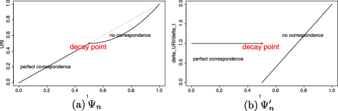
Figure 1: An illustration of the correspondence profile in an idealized case, where top 50% are genuine signals and bottom 50% are noise. In this case, all signals are ranked higher than noise; two rank lists have perfect correspondence for signals and no correspondence for noise. (a) Correspondence curve. (b) Change of correspondence curve.

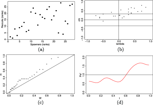
Figure 2: Rank scatterplot (a), Chi-plot (b), $K$-plot (c) and the change of correspondence curve (d) for salmon data, which consists of 28 measurements of size of the annual spawning stock of salmon and corresponding production of new catchable-sized fish in the Skeena River. The curve of $\Psi_{n}^{\prime}$ is produced by taking derivative on the spline that fits $\Psi_{n}$ with df${}={}$6.4.

We now compare the $\Psi_{n}^{\prime}$ plot with the Chi-plot and the $K$-plot using a real example considered in Kallenberg and Ledwina (1999), Fisher and Switzer (2001), Genest and Boies (2003). This data set consists of 28 measurements of size of the annual spawning stock of salmon and corresponding production of new catchable-sized fish in the Skeena River. It was speculated by Fisher and Switzer (2001) to contain a mixed populations with heterogeneous association. Though the dissimilarity of Chi-plot or $K$-plot to their prototypical plots [cf. Fisher and Switzer (2001); Genest and Boies (2003)] suggests the data may involve more than simple monotone association [Fisher and Switzer (2001); Genest and Boies (2003)], neither of these plots manifest heterogeneity of association. In the $\Psi^{\prime}_{n}$ curve [Figure 2(d)], the characteristic pattern of transition is observed at about $t=0.5$, which indicates that the data is likely to consist of two groups, with roughly the top 50% from a strongly associated group and the bottom 50% from a weakly associated group. It agrees with the speculation in Fisher and Switzer (2001).

2.2 Inferring the reproducibility of signals

In this section we present a statistical model that quantifies the dependence structure and infers the reliability of signals. Throughout this section, we will suppose, for simplicity, that we are dealing with a sample of i.i.d. observations from a population. Though this is in fact unrealistic in many applications, in particular, for the signals from genome-wide profiling (e.g., ChIP-seq experiments), where observations are often dependent, the descriptive and graphical value of our method remains, as we are concerned with first order effects.

In general, genuine signals tend to be more reproducible and score higher than spurious ones. The scores on replicates may be viewed as a mixture of two groups, which differ in both the strength of association and the level of significance. Recall that in these applications, the distributions and the scales of scores are usually unknown and may vary across data sets. To model such data, a semiparametric copula model is appropriate, in which the associations among the variables are represented by a simple parametric model but the marginal distributions are estimated nonparametrically using their ranks to permit arbitrary scales. Though using ranks, instead of the raw values of scores, generally causes some loss of information, this loss is known to be asymptotically negligible [Lehmann (2006)]. In view of the heterogeneous association in the genuine and spurious signals, we further model the heterogeneity of the dependence structure in the copula model using a mixture model framework.

Before proceeding to our model, we first provide a brief review of copula models, and refer to Joe (1997) and Nelson (1999) for a modern treatment of copula theory.

2.2.1 Copulas

The multivariate function $C=C(u_{1},\ldots,u_{p})$ is called a copula if it is a continuous distribution function and each marginal is a uniform distribution function on $[0,1]$. That is, $C\dvtx[0,1]^{p}\rightarrow[0,1]$, with $C(u)=P(U_{1}\leq u_{1},\ldots,U_{p}\leq u_{p})$, in which each $U_{j}\sim\operatorname{Unif}[0,1]$ and $u=(u_{1},\ldots,u_{p})$. By Sklar’s theorem [Sklar (1959)], every continuous multivariate probability distribution can be represented by its univariate marginal distributions and a copula, described using a bivariate case as follows.

Let $X_{1}$ and $X_{2}$ be two random variables with continuous CDFs $F_{1}$ and $F_{2}$. The copula $C$ of $X_{1}$ and $X_{2}$ can be found by making the marginal probability integral transforms on $X_{1}$ and $X_{2}$ so that

$$C(u_{1},u_{2})=F(F_{1}^{-1}(u_{1}),F_{2}^{-1}(u_{2})),\qquad u_{1},u_{2}\in[0,1],$$ (3)

where $F$ is the joint distribution function of $(X_{1},X_{2})$, $F_{1}$ and $F_{2}$ are the marginal distribution functions of $X_{1}$ and $X_{2}$, respectively, and $F_{1}^{-1}$ and $F_{2}^{-1}$ are the right-continuous inverses of $F_{1}$ and $F_{2}$, defined as $F_{j}^{-1}(u)=\operatorname{inf}\{z\dvtx\break F_{j}(z)\geq u\}$. That is, the copula is the joint distribution of $F_{1}(X_{1})$, $F_{2}(X_{2})$. These variables are unobservable but estimable by the normalized ranks $F_{n1}(X_{1})$, $F_{n2}(X_{2})$ where $F_{n1}$, $F_{n2}$ are the empirical distribution functions of the sample. The function $\delta_{C}(t,t)=C(t,t)$ is usually referred to as the diagonal section of a copula $C$. We will use the survival function of the copula $C$, $\bar{C}(u_{1},u_{2})=P(U_{1}>1-u_{1},U_{2}>1-u_{2})$, which describes the relationship between the joint survival function [$\bar{F}(x_{1},x_{2})=P(X_{1}>x_{1},X_{2}>x_{2})$] and its univariate margins ($\bar{F}_{j}=1-F_{j}$) in a manner completely analogous to the relationship between univariate and joint functions, as $\bar{C}(u_{1},u_{2})=\bar{F}(\bar{F}_{1}^{-1}(u_{1}),\bar{F}_{2}^{-1}(u_{2}))$. The sample version of (3) is called an empirical copula [Deheuvels (1979); Nelson (1999)], defined as

$$C_{n}\biggl{(}\frac{i}{n},\frac{j}{n}\biggr{)}=\frac{1}{n}\sum_{k=1}^{n}1\bigl{(}x_{k,1}\leq x_{(i),1},x_{k,2}\leq x_{(j),2}\bigr{)},\qquad 1\leq i,j\leq n,$$ (4)

for a sample of size $n$, where $x_{(i),1}$ and $x_{(j),2}$ denote order statistics on each coordinate from the sample. The sample version of survival copulas follows similarly.

This representation provides a way to parametrize the dependence structure between random variables separately from the marginal distributions, for example, a parametric model for the joint distribution of $u_{1}$ and $u_{2}$ and a nonparametric model for marginals. Copula-based models are natural in situations where learning about the association between the variables is important, but the marginal distributions are assumably unknown. For example, the 2-dimensional Gaussian copula $C$ is defined as

$$C(u_{1},u_{2}|\rho)=\Phi_{2}(\Phi^{-1}(u_{1}),\Phi^{-1}(u_{2})|\rho),$$ (5)

where $\Phi$ is the standard normal cumulative distribution function, $\Phi_{2}(\cdot,\cdot|\rho)$ is the cumulative distribution function for a bivariate normal vector $(z_{1},z_{2})\sim N\left(\left(0\atop 0\right),\left({1\atop\rho}\enskip{\rho\atop 1}\right)\right)$, and $\rho$ is the correlation coefficient. Modeling dependence with arbitrary marginals $F_{1}$ and $F_{2}$ using the Gaussian copula (5) amounts to assuming data is generated from latent variables $(z_{1},z_{2})$ by setting $x_{1}=F_{1}^{-1}(\Phi(z_{1}))$ and $x_{2}=F_{2}^{-1}(\Phi(z_{2}))$. Note that if $F_{1}$ and $F_{2}$ are not continuous, $u_{1}$ and $u_{2}$ are not uniform. For convenience, we assume that $F_{1}$ and $F_{2}$ are continuous throughout the text.

2.2.2 A copula mixture model

We now present our model for quantifying the dependence structure and inferring the reproducibility of signals. We assume throughout this part that our data is a sample of i.i.d. bivariate vectors $(x_{i,1},x_{i,2})$.

We assume the data consists of genuine signals and spurious signals, which in general correspond to a more reproducible group and a less reproducible group. We use the indicator $K_{i}$ to represent whether a signal $i$ is genuine ($K_{i}=1$) or spurious ($K_{i}=0$). Let $\pi_{1}$ and $\pi_{0}=1-\pi_{1}$ denote the proportion of genuine and spurious signals, respectively. Given $K_{i}=1$, we assume the pairs of scores for genuine (resp., spurious) signals are independent draws from a continuous bivariate distribution with density $f_{1}(\cdot,\cdot)$ [resp., $f_{0}(\cdot,\cdot)$, given $K_{i}=0$] with joint distribution $F_{1}(\cdot,\cdot)$ [resp., $F_{0}(\cdot,\cdot)$]. Note, however, that even if the marginal scales are known, $K_{i}$ would be unobservable so that the copula is generated by the marginal mixture (with respect to $K_{i}$), $F_{j}=\pi_{0}F_{j}^{0}+\pi_{1}F_{j}^{1}$, where $F_{j}$ is the marginal distribution of the $j$th coordinate and $F_{j}^{k}$ is the marginal distribution of the corresponding $k$th component.

Because genuine signals generally are more significant and more reproducible than spurious signals, we expect the two groups to have both different means and different dependence structures between replicates. We assume that, given the indicator $K_{i}$, the dependence between replicates for genuine (resp., spurious) signals is induced by a bivariate Gaussian distribution $\mathbf{z}_{1}=(z_{1,1},z_{1,2})$ [or resp., $\mathbf{z}_{0}=(z_{0,1},z_{0,2})$]. The choice of Gaussian distribution for inducing the dependence structure in each component is made based on the observation that the dependence within a component in the data we consider generally is symmetric and that an association parameter with a simple interpretation, such as the correlation coefficient for a Gaussian distribution, is natural.

As the scores from $F_{1}(\cdot,\cdot)$ are expected to be higher than the scores from $F_{0}(\cdot,\cdot)$, we assume $\mathbf{z}_{1}$ has a higher mean than $\mathbf{z}_{0}$. Since spurious signals are presumably less reproducible, we assume corresponding signals on the replicates to be independent, that is, $\rho_{0}=0$; whereas, since genuine signals usually are positively associated between replicates, we expect $\rho_{1}>0$, though $\rho_{1}$ is not required to be positive in our model. It also seems natural to assume that the underlying latent variables, reflecting replicates, have the same marginal distributions. Finally, we note that if the marginal scales are unknown, we can only identify the difference in means of the two latent variables and the ratio of their variances, but not the means and variances of the latent variables. Thus, the parametric model generating our copula can be described as follows:

Let $K_{i}\sim\operatorname{Bernoulli}(\pi_{1})$ and $(z_{i,1},z_{i,2})$ be distributed as

$$\pmatrix{z_{i,1}\cr z_{i,2}}\Bigm{|}K_{i}=k\sim N\left(\pmatrix{\mu_{k}\cr\mu_{k}},\pmatrix{\displaystyle\sigma_{k}^{2}&\rho_{k}\sigma_{k}^{2}\vspace*{1pt}\cr\displaystyle\rho_{k}\sigma_{k}^{2}&\sigma_{k}^{2}}\right),\qquad k=0,1,$$ (6a)

where $$\mu_{0}=0 \mu_{1}>0 \sigma_{0}^{2}=1 \rho_{0}=0 0<\rho_{1}\leq 1$$, , , , .

Let

$$u_{i,1} \equiv G(z_{i,1})=\frac{\pi_{1}}{\sigma_{1}}\Phi\biggl{(}\frac{z_{i,1}-\mu_{1}}{\sigma_{1}}\biggr{)}+\pi_{0}\Phi(z_{i,1}),$$

$$u_{i,2} \equiv G(z_{i,2})=\frac{\pi_{1}}{\sigma_{1}}\Phi\biggl{(}\frac{z_{i,2}-\mu_{1}}{\sigma_{1}}\biggr{)}+\pi_{0}\Phi(z_{i,2}).$$

Our actual observations are

$$x_{i,1} = F_{1}^{-1}(u_{i,1}),$$

$$x_{i,2} = F_{2}^{-1}(u_{i,2}),$$

where $F_{1}$ and $F_{2}$ are the marginal distributions of the two coordinates, which are assumed continuous but otherwise unknown.

Thus, our model, which we shall call a copula mixture model, is a semiparametric model parametrized by $\theta=(\pi_{1},\mu_{1},\sigma_{1}^{2},\rho_{1})$ and $(F_{1},F_{2})$. The corresponding mixture likelihood for the data is

$$L(\theta) = \prod_{i=1}^{n}[\pi_{0}h_{0}(G^{-1}(F_{1}(x_{i,1})),G^{-1}(F_{2}(x_{i,2})))$$ (7a)

$$\hphantom{\prod_{i=1}^{n}[}{}+\pi_{1}h_{1}(G^{-1}(F_{1}(x_{i,1})),G^{-1}(F_{2}(x_{i,2})))]$$

$$= \prod_{i=1}^{n}[c(F_{1}(x_{i,1}),F_{2}(x_{i,2}))g(G^{-1}(F_{1}(x_{i,1})))g(G^{-1}(F_{2}(x_{i,2})))],$$ (7b)

where

$$c(u_{1},u_{2})=\frac{\pi_{0}h_{0}(G^{-1}(u_{1}),G^{-1}(u_{2}))+\pi_{1}h_{1}(G^{-1}(u_{1}),G^{-1}(u_{2}))}{g(G^{-1}(u_{1}))g(G^{-1}(u_{2}))}$$ (7)

is a copula density function with

$$h_{0}\sim N\left(\left(\matrix{0\cr 0}\right),\left(\matrix{1&0\cr 0&1}\right)\right)\quad\mbox{and}\quad h_{1}\sim N\left(\left(\matrix{\mu_{1}\cr\mu_{1}}\right),\left(\matrix{\sigma_{1}^{2}&\rho_{1}\sigma_{1}^{2}\vspace*{1pt}\cr\rho_{1}\sigma_{1}^{2}&\sigma_{1}^{2}}\right)\right),$$

$G$ is defined in (2.2.2) and $g$ is the density function of $G$. Note that $G$ depends on $\theta$.

Given the parameters $\theta$, the posterior probability that a signal $i$ is in the irreproducible group can be computed as

$$\qquad\operatorname{Pr}\bigl{(}K_{i}=0\mid(x_{i1},x_{i2});\theta\bigr{)}=\frac{\pi_{0}h_{0}(G^{-1}(F_{1}(x_{i,1}),G^{-1}(F_{2}(x_{i,2}))))}{\sum_{k=0,1}\pi_{k}h_{k}(G^{-1}(F_{1}(x_{i,1}),G^{-1}(F_{2}(x_{i,2}))))}.$$ (8)

We estimate values for these classification probabilities by estimating the parameters $\theta$ using an estimation procedure described in Section 2.2.3, and substituting these estimates into the above formulas.

The idea of using a mixture of copulas to describe complex dependence structures is not entirely new. For example, the mixed copula model [Hu (2006)] in economics uses a mixture of copulas [$C_{\mathit{mix}}(u_{1},u_{2}\mid(\theta_{1},\ldots,\theta_{k}))=\sum_{i=1}^{k}C(u_{1},u_{2}\mid\theta_{i})$] to generate flexible fits to the dependence structures that do not follow any standard copula families. In this model, all the copulas in $C_{\mathit{mix}}$ are assumed to have identical marginal distributions. In contrast, the copula in our model not only has mixed associations, but also allows different associations to occur with different marginal distributions ($F_{j}^{0}$ and $F_{j}^{1}$), thus can be viewed as a generalization of the case with the same marginal distribution. In addition, our modeling goal is to cluster the observations into groups with homogeneous associations, instead of data fitting. This difference in marginal distributions calls for nonstandard estimation, which we expect to be efficient, as we shall see in Section 2.2.3.

2.2.3 Estimation of the copula mixture model

In this section we describe an estimation procedure that estimates the parameters $\theta$ in (7) and the membership $K_{i}$ of each observation.

A common strategy to estimate the association parameters in semiparametric copula models is a “pseudo-likelihood” approach, which is described in broad, nontechnical terms by Oakes (1994). In this approach, the empirical marginal distribution functions $\hat{F}_{j}$, after rescaling by multiplying by ($\frac{n}{n+1}$) to avoid infinities, are plugged into the copula density in (7b), ignoring the terms involving $g$. The association parameters are then estimated by maximizing the pseudo-copula likelihood. Genest, Ghoudi and Rivest (1995) showed, without specifying the algorithms to compute them, that under certain technical conditions, the estimators obtained from this approach are consistent, asymptotically normal, and fully efficient only if the coordinates of the copula are independent.

We adopt a different approach which, in principle, leads to efficient estimators under any choice of parameters and $F_{1}$, $F_{2}$. Note that the estimation of the association parameter $\rho_{1}$ depends on the estimation of $\mu_{1},\sigma_{1}^{2}$ and $\pi_{1}$ due to the presence of the mixture structure on marginal distributions, which makes the log-likelihood (7) difficult to maximize directly. Our approach is to estimate the parameters $\hat{\theta}$ by maximizing the log-likelihood (7) of pseudo-data $G^{-1}(\frac{n}{n+1}\hat{F}_{i,j};\theta)$, where $\hat{F}_{i,j}\equiv\hat{F}_{j}(x_{i,j})$.

As the latent variables $z_{0,j}$ and $z_{1,j}$ in our model form a mixture distribution, it is natural to use an expectation–maximization (EM) algorithm [Dempster, Laird and Rubin (1977)] to estimate the parameters $\hat{\theta}$ and infer the status of each putative signal for pseudo-data. In our approach, we first compute the pseudo-data $G^{-1}(\frac{n}{n+1}\hat{F}_{i,j};\theta_{0})$ from some initialization parameters $\theta^{(0)}$, then iterate between two stages: (1) maximizing $\theta$ based on the pseudo-data using EM and (2) updating the pseudo-data. The detailed procedure is given in the supplementary materials [Li et al. (2011)]. The EM stage may be trapped in local maxima, and the stage of updating pseudo-data may not converge from all starting points. However, in the simulations we performed (Section 3), it behaves well and finds the global maxima, when started from a number of initial points.

We sketch in the supplementary materials [Li et al. (2011), Section 2] a heuristic argument that a limit point of our algorithm close to the true value satisfies an equation whose solution is asymptotically efficient. Although our algorithm converges in practice, we have yet to show its convergence in theory. However, a modification which we are investigating does converge to the fixed point mentioned above. This work will appear elsewhere.

2.3 Irreproducible identification rate

In this section we derive a reproducibility criterion from the copula mixture model in Section 2.2.2 based on an analogy between our method and the multiple hypothesis testing problem. This criterion can be used to assess the reproducibility of both individual signals and the overall replicate outputs.

In the multiple hypothesis testing literature, the false discovery rate (FDR) and its variants, including positive false discovery rate (pFDR) and marginal false discovery rate (mFDR), are introduced to control the number of false positives in the rejected hypotheses [Benjamini and Hochberg (1995); Storey (2002); Genovese and Wasserman (2002)]. In the FDR context, when hypotheses are independent and identical, the test statistics can be viewed as following a mixture distribution of two classes, corresponding to whether or not the statistic is generated according to the null hypothesis [e.g., Efron (2004); Storey (2002)]. Based on this mixture model, the local false discovery rate, which is the posterior probability of being in the null component $\operatorname{Lfdr}(\cdot)=(1-\pi)f_{0}(\cdot)/f(\cdot)$, was introduced to compute the individual significance level [Efron (2004)]. Sun and Cai (2007) show, again for the i.i.d. case, that Lfdr is also an optimal statistic in the sense that the thresholding rule based on Lfdr controls the marginal false discovery rate with the minimum marginal false nondiscovery rate.

As in multiple hypothesis testing, we also build our approach on a mixture model and classify the observations into two classes. However, the two classes have different interpretation and representation: The two classes represent irreproducible measurements and reproducible measurements in our model, in contrast to nulls and nonnulls in the multiple testing context, respectively.

In analogy to the local false discovery rate, we define a quantity, which we call the local irreproducible discovery rate, to be

$$\operatorname{idr}(x_{i,1},x_{i,2})=\frac{\pi_{0}h_{0}(G^{-1}(F_{1}(x_{i,1})),G^{-1}(F_{2}(x_{i,2})))}{\sum_{k=0,1}\pi_{k}h_{k}(G^{-1}(F_{1}(x_{i,1})),G^{-1}(F_{2}(x_{i,2})))}.$$ (9)

This quantity can be thought of as the a posteriori probability that a signal is not reproducible on a pair of replicates [i.e., (8)], and can be estimated from the copula mixture model.

Similarly, we define the irreproducible discovery rate (IDR) in analogy to the mFDR,

$$\operatorname{IDR}(\gamma) = P(\mathit{irreproducible}\mid i\in I_{\gamma})$$

$$= \frac{\pi_{0}\int_{I_{\gamma}}dH_{0}(G^{-1}(F_{1}(x_{i,1})),G^{-1}(F_{2}(x_{i,2})))}{\int_{I_{\gamma}}dH(G^{-1}(F_{1}(x_{i,1})),G^{-1}(F_{2}(x_{i,2})))},$$

where $I_{\gamma}=\{(x_{i,1},x_{i,2})\dvtx\operatorname{idr}(x_{i,1},x_{i,2})<\gamma\}$, $H_{0}$ and $H$ are the CDF of density functions $h_{0}$ and $h=\pi_{0}h_{0}+\pi_{1}h_{1}$, respectively. For a desired control level $\alpha$, if $(x_{(i),1},x_{(i),2})$ are the pairs ranked by $\mathit{idr}$ values, define $l=\max\{i\dvtx\frac{1}{i}\sum_{j=1}^{i}\mathit{idr}_{j}\leq\alpha\}$. By selecting all $(x_{(i),1},x_{(i),2})$ ($i=1,\ldots,l$), we can think of this procedure as giving an expected rate of irreproducible discoveries no greater than $\alpha$. It is analogous to the adaptive step-up procedure of Sun and Cai (2007) for the multiple testing case.

This procedure essentially amounts to re-ranking the identifications according to the likelihood ratio of the joint distribution of the two replicates. The resulting rankings are generally different from the ranking of the original significance scores on either replicate.

Unlike the multiple testing procedure, our procedure does not require $x_{i,j}$ to be $p$-values; instead, $x_{i,j}$ can be any scores with continuous marginal distributions. When $p$-values are used as scores, our method can also be viewed as a method to combine $p$-values. We compare our method and two commonly-used $p$-value combinations through simulations in Section 3.

3 Simulation studies

3.1 Illustration of correspondence curves

To show the prototypical plots of more realistic cases, we use simulated data to compare and contrast the curves in presence and absence of the transition of association described in Section 2.1. (Figure 3). The case where no transition occurs is illustrated using two single-component bivariate Gaussian distributions with homogeneous association, $\rho=0$ [Figure 3(a)] and $\rho=0.8$ [Figure 3(b)], respectively. The presence of the transition is illustrated using two two-component bivariate Gaussian mixtures, whose lower ranked component has independent coordinates (i.e., $\rho_{0}=0$) and the higher ranked component has positively correlated coordinates with $\rho_{1}=1$ [Figure 3(c)] and $\rho_{1}=0.8$ [Figure 3(d)], respectively.

As in the idealized example (Figure 1), the characteristic transition of curves is observed when the transition of association is present [Figure 3(c), (d)], but not seen when the data consists of only one component with homogeneous association. This shows that the transition of the shape of the curve may be used as an indicator for the presence of the transition of association.

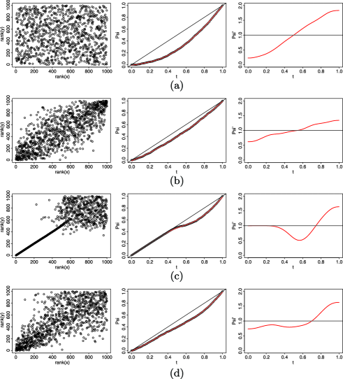
Figure 3: Behavior of correspondence curves when data consists of homogeneous and heterogeneous association. From left to right, the three columns are the scatterplot of ranks, the curve of $\Psi$ and the curve of $\Psi^{\prime}$. (a) Bivariate Gaussian distribution with $\rho=0$. (b) Bivariate Gaussian distribution with $\rho=0.8$. (c) A mixture of two bivariate Gaussian distributions with marginals on both coordinates as $f_{0}=N(0,1)$ and $f_{1}=N(3,1)$, $\rho_{0}=0$ and $\rho_{1}=1$ and mixing proportion $\pi_{1}=0.5$. (d) A mixture of two bivariate Gaussian distributions with marginals on both coordinates as $f_{0}=N(0,1)$ and $f_{1}=N(2,1)$, $\rho_{0}=0$ and $\rho_{1}=0.8$ and mixing proportion $\pi_{1}=0.5$. The curve of $\Psi_{n}^{\prime}$ is produced by taking the derivative on the spline that fits $\Psi_{n}$ with df${}={}$6.4.

3.2 Copula mixture model

We first use simulation studies to examine the performance of our approach. In particular, we aim to assess the accuracy of our classification, to evaluate the benefit of combining information between replicates over using only information on one replicate, and to assess the robustness of our method to the violation of one of its underlying model assumptions. In each simulation, we also compare the performance with two existing methods for combining significance scores across samples. However, as existing combination methods can be applied to only $p$-values, we use $p$-values as the significance scores in the comparison, though our method can be applied to arbitrary scores with continous marginal distributions. Here we consider the scenario when the $p$-values are not well calibrated but are reflective of the relative strength of evidence that the signals are real, and assess the accuracy of thresholds selected by all methods of comparison. These simulations also provide a helpful check on the convergence of our estimation procedure.

In each simulation study, we generate a sample of $n$ pairs of signals on two replicates. Each pair of observed signals $(Z_{i1},Z_{i,2})$ ($i=1,\ldots,n$) is a noisy realization of a latent signal $Z_{i}$, which is independently and identically generated from the following normal mixture model:

$$\displaystyle K_{i}\sim\operatorname{Bernoulli}(\pi_{1}),$$

$$\displaystyle Z_{i}\mid K_{i}=k\sim N(\mu_{k},\tau_{k}^{2}),\qquad k=0,\ldots,K-1,$$

$$\displaystyle Z_{i,j}\mid K_{i}=k,Z_{i}=Z_{i}+\varepsilon_{ijk},\qquad j=1,2,$$

$$\displaystyle\varepsilon_{ijk}\sim N(0,\omega_{k}^{2}).$$

As can easily be seen from the joint distribution of $(Z_{i,1},Z_{i,2})\mid K_{i}$,

$$\pmatrix{Z_{i,1}\cr Z_{i,2}}\Bigm{|}K_{i}=k\sim N\left(\pmatrix{\mu_{k}\cr\mu_{k}},\pmatrix{\displaystyle\tau_{k}^{2}+\omega_{k}^{2}&\rho_{k}(\tau_{k}^{2}+\omega_{k}^{2})\cr\displaystyle\rho_{k}(\tau_{k}^{2}+\omega_{k}^{2})&\tau_{k}^{2}+\omega_{k}^{2}}\right),$$

$$\eqntext{k=0,\ldots,K-1,}$$ (12)

where $\rho_{k}=\frac{\tau_{k}^{2}}{\tau_{k}^{2}+\omega_{k}^{2}}$; this model is in fact a reparameterization of our model (6a) when $K=2$: $(Z_{i,1},Z_{i,2})$ directly corresponds to the latent Gaussian variables in (6a) when setting $\mu_{0}=0,\mu_{1}>0,\tau^{2}_{k}+\omega_{k}^{2}=1,\rho_{0}=0$ and $k=0,1$. When $K>2$, this model is convenient for simulating data from multiple components and investigating the robustness of our method to the violation of the assumption that the data consists of a reproducible and an irreproducible component. After $Z_{i,j}$ is simulated, we transform $Z_{i,j}$ to a Student’s $t$ distribution by a probability integral transformation $F_{t_{5}}^{-1}(G(Z_{i,j}))$, where $F_{t_{5}}$ is the cdf of $t$ distribution with $\mathit{df}=5$ and $G$ is as defined in (2.2.2). We then obtain $p$-values from a one-sided $z$-test for $H_{0}\dvtx\mu=0$ vs $H_{1}\dvtx\mu>0$, and use them as the significance score $X_{i,j}$. This procedure is equivalent to applying a $z$-test to a t distribution, thus generating $p$-values that are not calibrated but are reflective of the relative strength of evidence that the signals are real. It is equivalent to letting $F_{j}^{-1}(\cdot)=1-\Phi(F_{t_{5}}^{-1}(\cdot))$ in (2.2.2) for our model.

With $p$-values as the significance score, our method can also be viewed as a way to combine $p$-values for ranking signals by their consensus. The two most commonly-used methods for combining $p$-values of a set of independent tests are Fisher’s combined test [Fisher (1925)] and Stouffer’s $z$ method [Stouffer et al. (1949)]. In Fisher’s combination for the given one-sided test, the test statistic $Q_{i}=-2\sum_{j=1}^{m}\log(p_{i,j})$ for each pair of signals has the $\chi^{2}_{2m}$ distribution under $H_{0}$, where $p_{i,j}$ is the $p$-value for the $i$th signal on the $j$th replicate, $m$ is the number of studies and $m=2$ here. In Stouffer’s method, the test statistic $S_{i}=\frac{1}{\sqrt{m}}\sum_{j=1}^{m}\Phi^{-1}(1-p_{i,j})$ has distribution $N(0,1)$ under $H_{0}$, where $\Phi$ is the standard normal CDF. For each pair of signals, we compute $Q_{i}$ ($S_{i}$, resp.) and its corresponding $p$-values $p^{Q}_{i}$ ($p^{S}_{i}$, resp.), then estimate the corresponding false discovery rates (FDR) by computing $q$-values [Storey (2003)] based on $p^{Q}_{i}$ ($p^{S}_{i}$, resp.), using R package “qvalue.” FDR is estimated similarly for $p$-values on the individual replicates.

For our method, we classify a call as correct (or incorrect), when a genuine (or spurious) signal is assigned an idr value smaller than an idr threshold. Correspondingly, for a call from individual replicates, Fisher’s method or Stouffer’s method, the same classification applies, when its corresponding $q$-value is smaller than the threshold. We compare the discriminative power of these methods by assessing the trade-off between the number of correct and incorrect calls made at various thresholds.

Table 1: Simulation parameters and parameter estimation in the simulation studies of 100 data sets. Each data set consists of 10,000 pairs of observations. The simulation parameters are estimated from a ChIP-seq data set. In all simulations, $\mu_{0}=0$, $\sigma_{0}^{2}=1$ and $\rho_{0}=0$. In S1–S3, $\pi_{0}=1-\pi_{1}$. S4 has a third component with $\mu_{2}=0$, $\sigma_{0}^{2}=1$, $\rho_{2}=0.64$, $\pi_{2}=0.07$ and $\pi_{0}=1-\pi_{1}-\pi_{2}$. The table shows the mean and the standard deviation of the estimated parameters over the 100 data sets using our model

		$\bolds{\pi_{1}}$	$\bolds{\rho_{1}}$	$\bolds{\mu_{1}}$	$\bolds{\sigma_{1}^{2}}$
S1	True parameter	0.650	0.840	2.500	1.000
	Estimated values	0.648 (0.005)	0.839 (0.005)	2.524 (0.033)	1.003 (0.024)
S2	True parameter	0.300	0.400	2.500	1.000
	Estimated values	0.302 (0.004)	0.398 (0.024)	2.549 (0.037)	1.048 (0.032)
S3	True parameter	0.050	0.840	2.500	1.000
	Estimated values	0.047 (0.004)	0.824 (0.026)	2.536 (0.110)	0.876 (0.087)
S4	True parameter	0.650	0.840	3.000	1.000
	Estimated values	0.669 (0.005)	0.850 (0.005)	3.021 (0.031)	1.058 (0.029)

In an attempt to generate realistic simulations, we first estimated parameters from a ChIP-seq data set (described in Section 4 using the model in Section 2.2), then simulated the signals on a pair of replicates using the sampling model (3.2). We performed four simulations, S1, S2, S3 and S4, as follows, with simulation parameters in Table 1:

1. [S3]

2. This simulation was designed to demonstrate performance when the data are generated from the same copula mixture model we use for estimation. Data were simulated from the model (3.2) with $K=2$, using the parameters estimated from the ChIP-seq data set considered below. The resulting data contained $\pi_{1}=65\%$ signals and $\pi_{0}=35\%$ noise.

3. A simulation to assess performance of our method when the correlation between genuine signals is low. Data were simulated as in S1 ($K=2$), except that $\rho_{1}=0.4$ and $\pi_{1}=0.3$.

4. A simulation to assess performance of our method when only a small proportion of real but highly correlated signals are present. Data were simulated as in S1 ($K=2$), except that $\pi_{1}=0.05$.

5. Here simulation parameters were chosen to illustrate a scenario when reproducible noise is present in addition to random noise and real signals. The goal is to assess the sensitivity of our method to deviations from the assumption that genuine signals are reproducible and noise is irreproducible. Data were simulated from a three-component model (i.e., $K=3$) using (3.2), where $\pi_{2}=7\%$ reproducible noise is added as the third component with $\rho_{2}=0.64$, $\mu_{2}=0$ and $\sigma_{2}^{2}=1$, and the parameters for signals and random noise are as in S1, except $\pi_{0}=28\%$ and $\mu_{1}=3$.

For each parameter set, we simulated 100 data sets, each of which consists of two replicates with 10,000 signals on each replicate. In each simulation, we ran the estimation procedure from 10 random initializations, and stopped the procedure when the increment of log-likelihood is $<$0.01 in an iteration or the number of iterations exceeds 100. All the simulations converge, when starting points are close to the true parameters. The results that converge to the highest likelihood are reported.

3.2.1 Parameter estimation and calibration of IDR

In S1–S3, the parameters estimated from our models are close to the true parameters (Table 1). The only exception is that $\sigma_{1}$ was underestimated when the proportion of true signals is small, $\pi_{1}=0.05$, a case hard to distinguish from that of a single component.

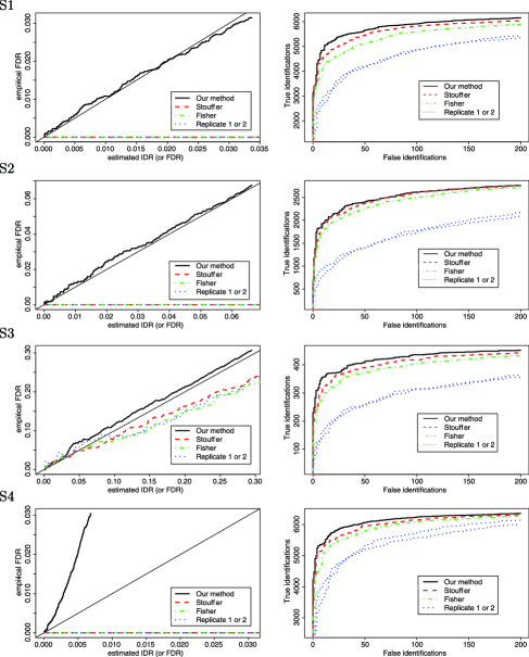
Figure 4: Calibration of IDR (Left) and comparison of discriminative power (Right) in simulation studies. Left: Estimated error rate ($x$-axis: IDR for our method and FDR for other methods) is compared with the actual frequency of false identifications ($y$-axis). Right: The number of correct and incorrect calls made at various thresholds in simulation studies. Incorrect calls: The number of spurious signals assigned idr values smaller than the thresholds (our method) or with $q$-values smaller than the cutoffs (other methods). Correct calls: The number of genuine signals assigned idr values smaller than the thresholds (our method) or with $q$-values smaller than the cutoffs (other methods).

The irreproducible discovery rate as a guide for the selection of the signals needs to be well calibrated. To check the calibration of thresholds, we compare the actual frequency of false calls, that is, empirical FDR, with the estimated IDR for our method and with the $q$-values for other methods (Figure 4, left column).

As shown in Figure 4, the original significance scores and other combination methods are overly conservative in their estimated FDR in all simulations, whereas our method is reasonably well calibrated in S1, S2 and S3. When reproducible noise is present (S4), our method slightly overestimates the proportion and the correlation of the real signals, and underestimates the empirical FDR (Figure 4-S4). This reflects that the data contains some artifacts that receive reproducible high scores on their original measures and consequently receive relatively low idr values. These artifacts are difficult to distinguish from genuine signals. We will compare the discriminative power of all four methods in the next section.

3.2.2 Comparison of discriminative power

To assess the benefit of combining information on replicates and compare with existing methods of combining $p$-values, we compared our method with the $p$-values on individual replicates, Fisher’s method and Stouffer’s method, by assessing the trade-off between the numbers of correct and incorrect calls made at various thresholds. As a small number of false calls is desired in practice, the comparison focuses on the performance in this region.

In all simulations, our method consistently identifies more true signals than the original significance score and the two $p$-value combination methods, at a given number of false calls in the studied region. Even when reproducible artifacts are present (S4) or only a small proportion of genuine signal is present (S3), our method still outperforms all methods compared here.

4 Applications on real data

4.1 Comparing the reproducibility of multiple peak callers for ChIP-seq experiments

We now consider an application arising from a collaborative project with the ENCODE consortium [ENCODE Project Consortium (2004)]. This project has three primary goals: comparing the reproducibility of multiple algorithms for identifying protein-binding regions in ChIP-seq data (described below), selecting binding regions using a uniform criterion for data from different sources (e.g., labs), and identifying experiment results in poor quality.

We now state the background of ChIP-Seq data in more detail and refer to Park (2009) for a recent review. A ChIP-seq experiment is a high-throughput assay to study protein binding sites on DNA sequences in a genome. In a typical ChIP-seq experiment, DNA regions that are specifically bound by the protein of interest are first enriched by immunoprecipitation, then the enriched DNA regions are sequenced by high-throughput sequencing, which generates a genome-wide scan of tag counts that correspond to the level of enrichment at each region. The relative significance of the regions are determined by a computational algorithm (usually referred to as a peak caller), largely according to local tag counts, based on either heuristics or some probabilistic models. The regions whose significance are above some prespecified threshold then are identified. To date, more than a dozen of the peak callers have been published. Some common measures of significance are fold enrichment, $p$-value or $q$-value [Storey (2003)].

Though these scores may reflect the relative strength of evidence for putative binding regions to be real, determination of a proper threshold is not straightforward, especially for heuristic-based scores, where arbitrary judgment often has to be involved. In fact, this difficulty could also exist for probabilistic-based scores if the underlying probabilistic models are inadequate to capture the complexity of the data. Because tuning parameters for each data set are usually infeasible due to lack of ground truth, default thresholds are often used in practice, though they may not be the optimal choices for the data to be analyzed. Ideally, an objective performance assessment should reflect the behavior of peak callers instead of the effect of thresholds.

Here we use the binding regions identified at untuned thresholds in a CTCF ChIP-seq experiment (described below) to illustrate how our method is used for assessing and comparing the reproducibility of peak callers when tuning thresholds are unavailable, for setting a reproducibility-based threshold that is appliable to both heuristic and probabilistic-based significance scores, and for identifying results with low reproducibility. A detailed analysis on a comprehensive set of ENCODE data will appear elsewhere.

4.1.1 Description of the data

In this comparison the ChIP-seq experiments of a transcription factor CTCF from two biological replicates were generated from the Bernstein Laboratory at the Broad Institute on human K526 cells. Peaks were identified in biology labs, using nine commonly used and publicly available peak callers, namely, Peakseq [Rozowsky et al. (2009)], MACS [Zhang et al. (2008)], SPP [Kharchenko, Tolstorukov and Park (2008)], Fseq [Boyle et al. (2008)], Hotspot [Thurman et al. (2011)], Erange [Mortazavi et al. (2008)], Cisgenome [Ji et al. (2008)], Quest [Valouev et al. (2008)] and SISSRS [Jothi et al. (2008)], using their default significance measures and default parameter settings with either default thresholds (all peak callers except Hotspot) or more relaxed thresholds (Hotspot). Among them, Peakseq and SPP use $q$-value, MACS, Hotspot and SISSRS use $p$-value, and the rest use fold enrichment, as their significance measures. Only the outputs from peak callers were available for our analysis.

The peaks generated from different algorithms have substantially different peak widths. SPP and SISSRS generate peaks with fixed width of 100 bp and 40 bp, respectively; all other algorithms generate peaks with varying peak width (median${}={}$130–760 bp). Because wider peaks are more likely to hit true binding sites by chance than shorter peaks, we normalized peak width by truncating the peaks wider than 40 bp down to intervals of 40 bp centered at the reported summits of peaks, so that reproducibility is compared on the same basis. The choice of 40 bp was made because the peak caller with the narrowest average peak width in our comparison reports peaks with a fixed width of 40 bp. Prior to applying our method, peaks on different replicates are paired as identifying the same binding region, if their coverage regions overlap (i.e., overlap $\geq$ 1 bp). Because peaks without matches do not have replicate measurements and are apparently irreproducible, here we elected to assess reproducibility of paired peaks in our analysis. Around 23–78% of peaks are retained for this analysis.

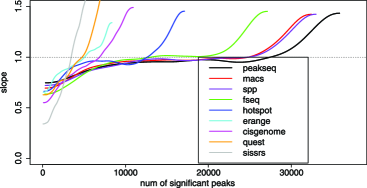
Figure 5: The change of correspondence ($\Psi_{n}^{\prime}$) along the decreasing order of significance, plotted for 9 peak callers on a CTCF ChIP-seq experiment from ENCODE. $X$-axis: The rank list of peaks identified on a replicate. $Y$-axis: $\Psi_{n}^{\prime}$.

4.2 Results

4.2.1 Correspondence profiles

Figure 5 shows the correspondence profiles for the nine peak callers. By referring to the prototypical plots in Figure 3, five peak callers (Peakseq, MACS, SPP, Fseq and Hotspot) show the characteristic transition from strong association to near independence [Figure 5(b)]. As described in Section 2.1, when heterogeneity of association is present, a high reproducibility translates to late occurrence of the transition to a segment with a positive slope. According to how much down the rank list the transition is observed, the three peak callers that show the highest reproducibility on this data set are Peakseq, MACS and SPP (Figure 5). For the other four peak callers (Erange, Cisgenome, Quest and SISSRS), the curves display a less clear transition and report substantially fewer (reproducible) peaks. This indicates that the default thresholds for these peak callers are likely to be too stringent to reach the breakdown of consistency, and that the reported peaks have relatively low reproducibility across replicates. This conclusion was confirmed later by biological verification (see Section 4.2.3).

4.2.2 Inference from the copula mixture model

We applied the copula mixture model to the peaks identified on the replicates for each peak caller. As data may consist of only one group with homogeneous association, we also estimated the fit using a one-component model that corresponds to setting $\pi_{1}=1,\mu_{1}=0$ and $\sigma_{1}^{2}=1$ in (6). We then tested for the smallest number of components compatible with the data, using a likelihood ratio test statistic ($\lambda=\frac{L_{2}}{L_{1}}$), where $L_{2}$ and $L_{1}$ are the likelihood of two-component and one-component models, respectively. With mixture models, it is well known that the regularity conditions do not hold for $2\log(\lambda)$ to have its usual asymptotic Chi-square null distribution. We therefore used a parametric bootstrap procedure to obtain appropriate $p$-values [McLachlan (1987)]. In our procedure, 100 bootstrap samples were sampled from the null distribution under the one component hypothesis using the parametric bootstrap, where the parameter estimate was obtained by maximizing the pseudo-likelihood of the data under the null hypothesis of the one-component model. Then $p$-values were obtained by referring to the distribution of the likelihood ratio computed from the bootstrap samples. Table 2 summarizes the parameter estimation from both models and the bootstrap results.

Based on the likelihood ratio test, it seems that the one-component model fits the results from SISSRS, Quest and Cisgenome better, and the two-component model fits the results from other peak callers. This is consistent with the pattern of transition in the correspondence profiles (Figure 5).

To select binding sites, we rank putative peaks by the values of local idr and compute the irreproducible discovery rate (IDR) for peaks selected at various local idr cutoffs using (2.3), as described in Section 2.3. We illustrate the IDR as a function of the numbers of top peaks (ranked by local idr) for all peak callers in Figure 6. For a given IDR level, one can determine the number of peaks to be called from this plot, regardless of what type of scores are used to measure the significance of peaks. For example, at $5\%$ IDR, the top 27,500 peaks with the smallest local idr can be called using MACS. Using the same reproducibility criterion, peaks can be selected for other peak callers similarly.

Table 2: Parameters estimated from the copula mixture model and the one-component model, and model selection for determining the number of components. $(\pi_{1},\rho_{1},\mu_{1},\sigma_{1})$ are parameters estimated from the copula mixture model; $\rho$ is estimated from the single-component model. The number of components is selected using a likelihood ratio test and the $p$-value of the test statistics is determined using a parametric bootstrap approach based on 100 bootstrap samples

	Peakseq	MACS	SPP	Fseq	Hotspot	Cisgenome	Erange	Quest	Sissrs
$\pi_{1}$	0.69	0.84	0.77	0.74	0.69	0.85	0.72	0.72	1.00
$\rho_{1}$	0.89	0.89	0.88	0.82	0.88	0.65	0.81	0.67	0.24
$\mu_{1}$	2.27	2.07	2.28	2.12	1.62	2.05	2.04	2.01	7.27
$\sigma_{1}$	0.87	1.34	1.05	0.86	0.64	1.35	0.90	1.39	0.03
$\rho$	0.87	0.87	0.86	0.83	0.78	0.66	0.80	0.66	0.23
$p$-value	0.00	0.00	0.00	0.00	0.00	1.00	0.00	1.00	1.00

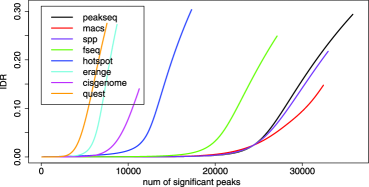
Figure 6: Irreproducible discovery rate (IDR) at different numbers of selected peaks, plotted at various idr cutoffs for eight peak callers on a CTCF Chip-seq experiment from ENCODE. Peaks are selected using local idr. $X$-axis: The rank list of peaks, ranked by local idr, $Y$-axis: Irreproducible discovery rate (IDR). SISSRS is not shown because its results are highly inconsistent and all peaks are grouped into a low correlation group.

We also compare the overall reproducibility of different peak callers using Figure 6. For example, while Peakseq, MACS and SPP on average have about $3\%$ irreproducible peaks when selecting the top 25,000 peaks, most of the other peak callers have already reached a much higher IDR before identifying the top 10,000 peaks. According to the number of peaks identified before reaching $5\%$ IDR, the three most reproducible peak callers on this data set are Peakseq, MACS and SPP, then followed by Fseq, then others. This result is consistent with the graphical comparison based on the correspondence profile (Figure 5).

4.2.3 Evaluating the biological relevance of the reproducibility assessment

To evaluate the biological relevance of our reproducibility assessment, we check the accuracy of peak identifications using external biological information. Because a complete list of true binding regions is not known for the examined data set, the accuracy of peak identifications is assessed using high-confidence binding motifs computationally predicted using sequence information [Kheradpour et al. (2007)], which is a commonly used device in this setting [e.g., Zhang et al. (2008); Kharchenko, Tolstorukov and Park (2008), among many others]. Though high-confidence motifs are not required to be bound and true binding sites are not required to exhibit a motif signature, the high-confidence motif instances are assumed, standard in this context, to contain a representative subset of true binding regions and are expected to have a relatively high occurrence in high-scored ChIP-seq peaks [Kharchenko, Tolstorukov and Park (2008)]. We selected ChIP-seq peaks reported by each peak caller at various IDR thresholds, and examined the number of high-confidence motifs (FDR $\leq 0.1$ at the PWM threshold of $p$-value${}=\frac{1}{4^{10}}$) that coincide with the reported ChIP-seq peaks (defined as overlap${}\geq 1$ bp) (Figure 7).

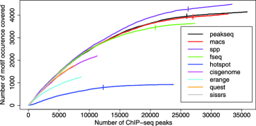
Figure 7: The coverage of high-confidence CTCF motif at different numbers of selected ChIP-seq peaks, plotted at various idr cutoffs for nine peak callers on a CTCF Chip-seq experiment from ENCODE. The bars on the curves of Peakseq, MACS, SPP, Fseq and Hotspot show the number of peaks selected at IDR${}={}$0.05. No selection is made for the rest of the peak callers because model selection favors the one-component model for peaks identified by these callers.

For the peak callers whose reported peaks fit the two-component model (i.e., Peakseq, MACS, SPP, Fseq and Hotspot), we marked the number of ChIP-seq peaks selected at IDR${}={}$5%. For these algorithms, the motif occurrences first increase with the increase of reported ChIP-seq peaks, then plateau before reaching the default thresholds (Figure 7). The mark of $5\%$ IDR approximately corresponds to the occurrences of the plateau, with few additional motif occurrences if more ChIP-seq peaks are called.

On the other hand, for the peak callers (Erange, Cisgenome, Quest and SISSRS) whose peaks fit the one-component model, the motif occurrence still shows an increasing trend at default thresholds. This confirms the observation from correspondence curves (Figure 5) that the default thresholds for these peak callers are likely to be overly stringent for this data set.

Overall, the results of this analysis agree with the assessment from our reproducibility comparison: the three peak calling results with the highest reproducibility (SPP, Peakseq and MACS) in Figure 6 show the highest rates of motif occurrence among all algorithms of comparison; the ones that are reported to be less reproducible do show lower rates of motif occurrence. This illustrates the potential of our method as a quality measure.

5 Discussion

We have presented a new statistical method for measuring the reproducibility of results in high-throughput experiments and setting selection thresholds using a reproducibility criterion. Using simulated and real data, we have illustrated the potential of our method for providing reproducibility assessment that is not confounded with prespecified threshold choices, determining biologically relevant thresholds, improving the accuracy of signal identification, and identifying suboptimal results.

As no assumption is made on the scale of the scores, the proposed method is applicable for any scoring system that produces continuous ranking to reflect the relative ordering of the signals. It provides a principled way to select signals that are scored on heuristic measures, and complements the thresholds determined on individual replicates. Moreover, because consistency between replicates is an internal standard that is independent of the scoring schemes and comparable across data sets, the proposed reproducibility criterion is suited for setting uniform standards for selecting signals for data from multiple sources, such as consortium studies. Because our measure of consistency is not confounded by platform-dependent thresholds, inter-platform consistency can be assessed easily.

Of course, reproducibility is only a necessary but not a sufficient condition to accuracy. If replicates are generated in the presence of a systematic bias that introduces false association, the threshold derived from this procedure may underestimate the empirical false discovery rate. Though the thresholds determined by our method show reasonable biological relevance in the data examined here and many other ENCODE ChIP-seq experiments (to appear in another manuscript), we emphasize that some cares are necessary to ensure that the replicates maintain the level of independence that they should.

We also note that the reproducibility of outputs from a data-analytical method (e.g., a peak caller) on replicate samples reflects the combined properties of the method and the samples. As the behavior of the data-analytical method may vary across different samples, the reproducibility assessment in our example should be interpreted as being specific to the studied data set, instead of a general conclusion. A detailed comparison of the performance of peak callers has been evaluated on a comprehensive set of data and will appear elsewhere.

The algorithm to implement the estimation strategy outlined in Section 2.2.3 is provided as supplemental material to this article. An R package is downloadable at the following website: http://cran.r-project.org/web/packages/idr/index.html.

Supplementary materials for Measuring reproducibility of high-throughput experiments [doi]10.1214/11-AOAS466SUPP [url]http://lib.stat.cmu.edu/aoas/466/supplement.pdf .pdf This supplement consists of four parts. Part 1 describes the algorithm for estimating parameters in our copula mixture model. Part 2 provides a theoretical justification for the efficiency of our estimator for the proposed copula mixture model when n is large. Part 3 derives the properties of the correspondence curves in Section 2.1.1. Part 4 provides an extension of our model to the case with multiple replicates.

References

- Benjamini and Hochberg (1995) {barticle}[mr] \bauthor\bsnmBenjamini, \bfnmYoav\binitsY. and \bauthor\bsnmHochberg, \bfnmYosef\binitsY. (\byear1995). \btitleControlling the false discovery rate: A practical and powerful approach to multiple testing. \bjournalJ. Roy. Statist. Soc. Ser. B \bvolume57 \bpages289–300. \bidissn=0035-9246, mr=1325392 \endbibitem
- Blest (2000) {barticle}[mr] \bauthor\bsnmBlest, \bfnmDavid C.\binitsD. C. (\byear2000). \btitleRank correlation—an alternative measure. \bjournalAust. N. Z. J. Stat. \bvolume42 \bpages101–111. \biddoi=10.1111/1467-842X.00110, issn=1369-1473, mr=1747465 \endbibitem
- Boulesteix and Slawski (2009) {barticle}[auto:STB—2011-03-03—12:04:44] \bauthor\bsnmBoulesteix, \bfnmA. L.\binitsA. L. and \bauthor\bsnmSlawski, \bfnmM.\binitsM. (\byear2009). \btitleStability and aggregation of ranked gene lists. \bjournalBriefings in Bioinformatics \bvolume10 \bpages556–568. \endbibitem
- Boyle et al. (2008) {barticle}[auto:STB—2011-03-03—12:04:44] \bauthor\bsnmBoyle, \bfnmA. P.\binitsA. P., \bauthor\bsnmGuinney, \bfnmJ.\binitsJ., \bauthor\bsnmCrawford, \bfnmG. E.\binitsG. E. and \bauthor\bsnmFurey, \bfnmT. S.\binitsT. S. (\byear2008). \btitleF-Seq: A feature density estimator for high-throughput sequence tags. \bjournalBioinformatics \bvolume24 \bpages2537–2538. \endbibitem
- da Costa and Soares (2005) {barticle}[mr] \bauthor\bparticleda \bsnmCosta, \bfnmJoaquim Pinto\binitsJ. P. and \bauthor\bsnmSoares, \bfnmCarlos\binitsC. (\byear2005). \btitleA weighted rank measure of correlation. \bjournalAust. N. Z. J. Stat. \bvolume47 \bpages515–529. \biddoi=10.1111/j.1467-842X.2005.00413.x, issn=1369-1473, mr=2235420 \endbibitem
- Deheuvels (1979) {barticle}[mr] \bauthor\bsnmDeheuvels, \bfnmPaul\binitsP. (\byear1979). \btitleLa fonction de dépendance empirique et ses propriétés. Un test non paramétrique d’indépendance. \bjournalAcad. Roy. Belg. Bull. Cl. Sci. (5) \bvolume65 \bpages274–292. \bidissn=0001-4141, mr=0573609 \endbibitem
- Dempster, Laird and Rubin (1977) {barticle}[mr] \bauthor\bsnmDempster, \bfnmA. P.\binitsA. P., \bauthor\bsnmLaird, \bfnmN. M.\binitsN. M. and \bauthor\bsnmRubin, \bfnmD. B.\binitsD. B. (\byear1977). \btitleMaximum likelihood from incomplete data via the EM algorithm. \bjournalJ. Roy. Statist. Soc. Ser. B \bvolume39 \bpages1–38. \bidissn=0035-9246, mr=0501537 \endbibitem
- Efron (2004) {bmisc}[auto:STB—2011-03-03—12:04:44] \bauthor\bsnmEfron, \bfnmB.\binitsB. (\byear2004). \bhowpublishedLocal false discovery rate. Technical report, Dept. Statistics, Stanford Univ. \endbibitem
- ENCODE Project Consortium (2004) {bmisc}[pbm] \borganizationENCODE Project Consortium (\byear2004). \bhowpublishedThe ENCODE (ENCyclopedia Of DNA Elements) Project. Science 306 636–640. \biddoi=10.1126/science.1105136, issn=1095-9203, pii=306/5696/636, pmid=15499007 \endbibitem
- Fisher (1925) {bbook}[auto:STB—2011-03-03—12:04:44] \bauthor\bsnmFisher, \bfnmR. A.\binitsR. A. (\byear1925). \btitleStatistical Methods for Research Workers, \bedition1st ed. \bpublisherOliver & Boyd, \baddressEdinburgh. \endbibitem
- Fisher and Switzer (1985) {barticle}[mr] \bauthor\bsnmFisher, \bfnmN. I.\binitsN. I. and \bauthor\bsnmSwitzer, \bfnmP.\binitsP. (\byear1985). \btitleChi-plots for assessing dependence. \bjournalBiometrika \bvolume72 \bpages253–265. \biddoi=10.1093/biomet/72.2.253, issn=0006-3444, mr=0801767 \endbibitem
- Fisher and Switzer (2001) {barticle}[mr] \bauthor\bsnmFisher, \bfnmN. I.\binitsN. I. and \bauthor\bsnmSwitzer, \bfnmP.\binitsP. (\byear2001). \btitleGraphical assessment of dependence: Is a picture worth 100 tests? \bjournalAmer. Statist. \bvolume55 \bpages233–239. \biddoi=10.1198/000313001317098248, issn=0003-1305, mr=1963399 \endbibitem
- Genest and Boies (2003) {barticle}[mr] \bauthor\bsnmGenest, \bfnmChristian\binitsC. and \bauthor\bsnmBoies, \bfnmJean-Claude\binitsJ.-C. (\byear2003). \btitleDetecting dependence with Kendall plots. \bjournalAmer. Statist. \bvolume57 \bpages275–284. \biddoi=10.1198/0003130032431, issn=0003-1305, mr=2016261 \endbibitem
- Genest, Ghoudi and Rivest (1995) {barticle}[mr] \bauthor\bsnmGenest, \bfnmC.\binitsC., \bauthor\bsnmGhoudi, \bfnmK.\binitsK. and \bauthor\bsnmRivest, \bfnmL. P.\binitsL. P. (\byear1995). \btitleA semiparametric estimation procedure of dependence parameters in multivariate families of distributions. \bjournalBiometrika \bvolume82 \bpages543–552. \biddoi=10.1093/biomet/82.3.543, issn=0006-3444, mr=1366280 \endbibitem
- Genest and Plante (2003) {barticle}[mr] \bauthor\bsnmGenest, \bfnmChristian\binitsC. and \bauthor\bsnmPlante, \bfnmJean-François\binitsJ.-F. (\byear2003). \btitleOn Blest’s measure of rank correlation. \bjournalCanad. J. Statist. \bvolume31 \bpages35–52. \biddoi=10.2307/3315902, issn=0319-5724, mr=1985503 \endbibitem
- Genovese and Wasserman (2002) {barticle}[mr] \bauthor\bsnmGenovese, \bfnmChristopher\binitsC. and \bauthor\bsnmWasserman, \bfnmLarry\binitsL. (\byear2002). \btitleOperating characteristics and extensions of the false discovery rate procedure. \bjournalJ. R. Stat. Soc. Ser. B Stat. Methodol. \bvolume64 \bpages499–517. \biddoi=10.1111/1467-9868.00347, issn=1369-7412, mr=1924303 \endbibitem
- Hu (2006) {barticle}[auto:STB—2011-03-03—12:04:44] \bauthor\bsnmHu, \bfnmL.\binitsL. (\byear2006). \btitleDependence patterns across financial markets: A mixed copula approach. \bjournalApplied Financial Economics \bvolume16 \bpages717–729. \endbibitem
- Ji et al. (2008) {barticle}[auto:STB—2011-03-03—12:04:44] \bauthor\bsnmJi, \bfnmH.\binitsH., \bauthor\bsnmJiang, \bfnmH.\binitsH., \bauthor\bsnmMa, \bfnmW.\binitsW., \bauthor\bsnmJohnson, \bfnmD. S.\binitsD. S., \bauthor\bsnmMyers, \bfnmR. M.\binitsR. M. and \bauthor\bsnmWong, \bfnmW. H.\binitsW. H. (\byear2008). \btitleAn integrated software system for analyzing ChIP-chip and ChIP-seq data. \bjournalNature Biotechnology \bvolume26 \bpages1293–1300. \endbibitem
- Joe (1997) {bbook}[mr] \bauthor\bsnmJoe, \bfnmHarry\binitsH. (\byear1997). \btitleMultivariate Models and Dependence Concepts. \bseriesMonogr. Statist. Appl. Probab. \bvolume73. \bpublisherChapman & Hall, \baddressLondon. \bidmr=1462613 \endbibitem
- Jothi et al. (2008) {barticle}[auto:STB—2011-03-03—12:04:44] \bauthor\bsnmJothi, \bfnmR.\binitsR., \bauthor\bsnmCuddapah, \bfnmS.\binitsS., \bauthor\bsnmBarski, \bfnmA.\binitsA., \bauthor\bsnmCui, \bfnmK.\binitsK. and \bauthor\bsnmZhao, \bfnmK.\binitsK. (\byear2008). \btitleGenome-wide identification of in vivo protein-DNA binding sites from ChIP-seq data. \bjournalNucleic Acids Res. \bvolume36 \bpages5221–5231. \endbibitem
- Kallenberg and Ledwina (1999) {barticle}[mr] \bauthor\bsnmKallenberg, \bfnmWilbert C. M.\binitsW. C. M. and \bauthor\bsnmLedwina, \bfnmTeresa\binitsT. (\byear1999). \btitleData-driven rank tests for independence. \bjournalJ. Amer. Statist. Assoc. \bvolume94 \bpages285–301. \bidissn=0162-1459, mr=1689233 \endbibitem
- Kharchenko, Tolstorukov and Park (2008) {barticle}[auto:STB—2011-03-03—12:04:44] \bauthor\bsnmKharchenko, \bfnmP. V.\binitsP. V., \bauthor\bsnmTolstorukov, \bfnmM. Y.\binitsM. Y. and \bauthor\bsnmPark, \bfnmP. J.\binitsP. J. (\byear2008). \btitleDesign and analysis of ChIP-seq experiments for DNA-binding proteins. \bjournalNature Biotechnology \bvolume26 \bpages1351–1359. \endbibitem
- Kheradpour et al. (2007) {barticle}[auto:STB—2011-03-03—12:04:44] \bauthor\bsnmKheradpour, \bfnmP.\binitsP., \bauthor\bsnmStark, \bfnmA.\binitsA., \bauthor\bsnmRoy, \bfnmS.\binitsS. and \bauthor\bsnmKellis, \bfnmM.\binitsM. (\byear2007). \btitleReliable prediction of regulator targets using 12 drosophila genomes. \bjournalGenome Res. \bvolume17 \bpages1919–1931. \endbibitem
- Kuo et al. (2006) {barticle}[auto:STB—2011-03-03—12:04:44] \bauthor\bsnmKuo, \bfnmW.\binitsW., \bauthor\bsnmLiu, \bfnmF.\binitsF., \bauthor\bsnmTrimarchi, \bfnmJ.\binitsJ., \bauthor\bsnmPunzo, \bfnmC.\binitsC., \bauthor\bsnmLombardi, \bfnmM.\binitsM., \bauthor\bsnmSarang, \bfnmJ.\binitsJ., \bauthor\bsnmWhipple, \bfnmM. E.\binitsM. E. \betalet al. (\byear2006). \btitleA sequence-oriented comparison of gene expression measurements across different hybridization-based technologies. \bjournalNature Biotechnology \bvolume24 \bpages832–840. \endbibitem
- Lehmann (2006) {bbook}[auto:STB—2011-03-03—12:04:44] \bauthor\bsnmLehmann, \bfnmErich L.\binitsE. L. (\byear2006). \btitleNonparametrics: Statistical Methods Based on Ranks, \bedition2nd ed. \bpublisherSpringer, \baddressNew York. \endbibitem
- Li et al. (2011) {bmisc}[auto:STB—2011-03-03—12:04:44] \bauthor\bsnmLi, \bfnmQ.\binitsQ., \bauthor\bsnmBrown, \bfnmJ. B.\binitsJ. B., \bauthor\bsnmHuang, \bfnmH.\binitsH. and \bauthor\bsnmBickel, \bfnmP. J.\binitsP. J. (\byear2011). \bhowpublishedSupplement to “Measuring reproducibility of high-throughput experiments.” DOI:10.1214/11-AOAS466SUPP. \endbibitem
- MAQC consortium (2006) {bmisc}[auto:STB—2011-03-03—12:04:44] \borganizationMAQC consortium (\byear2006). \bhowpublishedThe microarray quality control (MAQC) project shows inter- and intraplatform reproducibility of gene expression measurements. Nature Biotechnology 24 1151–1161. \endbibitem
- McLachlan (1987) {barticle}[auto:STB—2011-03-03—12:04:44] \bauthor\bsnmMcLachlan, \bfnmG. J.\binitsG. J. (\byear1987). \btitleOn bootstrapping the likelihood ratio test statistic for the number of components in a normal mixture. \bjournalApplied Statistics \bvolume36 \bpages318–324. \endbibitem
- Mortazavi et al. (2008) {barticle}[auto:STB—2011-03-03—12:04:44] \bauthor\bsnmMortazavi, \bfnmA.\binitsA., \bauthor\bsnmWilliams, \bfnmB. A.\binitsB. A., \bauthor\bsnmMcCue, \bfnmK.\binitsK., \bauthor\bsnmSchaeffer, \bfnmL.\binitsL. and \bauthor\bsnmWold, \bfnmB.\binitsB. (\byear2008). \btitleMapping and quantifying mammalian transcriptomes by RNA-seq. \bjournalNature Methods \bvolume5 \bpages621–628. \endbibitem
- Nelson (1999) {bbook}[auto:STB—2011-03-03—12:04:44] \bauthor\bsnmNelson, \bfnmR. B.\binitsR. B. (\byear1999). \btitleAn Introduction to Copulas, \bedition2nd ed. \bpublisherSpringer, \baddressNew York. \endbibitem
- Oakes (1994) {barticle}[mr] \bauthor\bsnmOakes, \bfnmDavid\binitsD. (\byear1994). \btitleMultivariate survival distributions. \bjournalJ. Nonparametr. Stat. \bvolume3 \bpages343–354. \biddoi=10.1080/10485259408832593, issn=1048-5252, mr=1291555 \endbibitem
- Park (2009) {barticle}[pbm] \bauthor\bsnmPark, \bfnmPeter J.\binitsP. J. (\byear2009). \btitleChIP-seq: Advantages and challenges of a maturing technology. \bjournalNat. Rev. Genet. \bvolume10 \bpages669–680. \biddoi=10.1038/nrg2641, issn=1471-0064, pii=nrg2641, pmid=19736561 \endbibitem
- Rozowsky et al. (2009) {barticle}[auto:STB—2011-03-03—12:04:44] \bauthor\bsnmRozowsky, \bfnmJ.\binitsJ., \bauthor\bsnmEuskirchen, \bfnmG.\binitsG., \bauthor\bsnmAuerbach, \bfnmR. K.\binitsR. K., \bauthor\bsnmZhang, \bfnmZ. D.\binitsZ. D., \bauthor\bsnmGibson, \bfnmT.\binitsT., \bauthor\bsnmBjornson, \bfnmR.\binitsR., \bauthor\bsnmCarriero, \bfnmN.\binitsN., \bauthor\bsnmSnyder, \bfnmM.\binitsM. and \bauthor\bsnmGerstein, \bfnmM. B.\binitsM. B. (\byear2009). \btitlePeakSeq enables systematic scoring of ChIP-seq experiments relative to controls. \bjournalNature Biotechnology \bvolume27 \bpages66–75. \endbibitem
- Sklar (1959) {barticle}[mr] \bauthor\bsnmSklar, \bfnmM.\binitsM. (\byear1959). \btitleFonctions de répartition à dimensions et leurs marges. \bjournalPubl. Inst. Statist. Univ. Paris \bvolume8 \bpages229–231. \bidmr=0125600 \endbibitem
- Storey (2002) {barticle}[mr] \bauthor\bsnmStorey, \bfnmJohn D.\binitsJ. D. (\byear2002). \btitleA direct approach to false discovery rates. \bjournalJ. R. Stat. Soc. Ser. B Stat. Methodol. \bvolume64 \bpages479–498. \biddoi=10.1111/1467-9868.00346, issn=1369-7412, mr=1924302 \endbibitem
- Storey (2003) {barticle}[mr] \bauthor\bsnmStorey, \bfnmJohn D.\binitsJ. D. (\byear2003). \btitleThe positive false discovery rate: A Bayesian interpretation and the -value. \bjournalAnn. Statist. \bvolume31 \bpages2013–2035. \biddoi=10.1214/aos/1074290335, issn=0090-5364, mr=2036398 \endbibitem
- Stouffer et al. (1949) {bmisc}[auto:STB—2011-03-03—12:04:44] \bauthor\bsnmStouffer, \bfnmS. A.\binitsS. A., \bauthor\bsnmSuchman, \bfnmE. A.\binitsE. A., \bauthor\bsnmDeVinney, \bfnmL. C.\binitsL. C., \bauthor\bsnmStar, \bfnmS. A.\binitsS. A. and \bauthor\bsnmWilliams, \bfnmJ.\binitsJ. (\byear1949). \bhowpublishedThe American Soldier: Vol. 1. Adjustment During Army Life. Princeton Univ. Press, Princeton, NJ. \endbibitem
- Sun and Cai (2007) {barticle}[mr] \bauthor\bsnmSun, \bfnmWenguang\binitsW. and \bauthor\bsnmCai, \bfnmT. Tony\binitsT. T. (\byear2007). \btitleOracle and adaptive compound decision rules for false discovery rate control. \bjournalJ. Amer. Statist. Assoc. \bvolume102 \bpages901–912. \biddoi=10.1198/016214507000000545, issn=0162-1459, mr=2411657 \endbibitem
- Thurman et al. (2011) {bmisc}[auto:STB—2011-03-03—12:04:44] \bauthor\bsnmThurman, \bfnmR.\binitsR., \bauthor\bsnmHawrylycz, \bfnmM.\binitsM., \bauthor\bsnmKuehn, \bfnmS.\binitsS., \bauthor\bsnmHaugen, \bfnmE.\binitsE. and \bauthor\bsnmStamatoyannopoulos, \bfnmS.\binitsS. (\byear2011). \bhowpublishedHotspot: A scan statistic for identifying enriched regions of short-read sequence tags. Unpublished manuscript, Univ. Washington. \endbibitem
- Valouev et al. (2008) {barticle}[auto:STB—2011-03-03—12:04:44] \bauthor\bsnmValouev, \bfnmA.\binitsA., \bauthor\bsnmJohnson, \bfnmD. S.\binitsD. S., \bauthor\bsnmSundquist, \bfnmA.\binitsA., \bauthor\bsnmMedina, \bfnmC.\binitsC., \bauthor\bsnmAnton, \bfnmE.\binitsE., \bauthor\bsnmBatzoglou, \bfnmS.\binitsS., \bauthor\bsnmMyers, \bfnmR. M.\binitsR. M. and \bauthor\bsnmSidow, \bfnmA.\binitsA. (\byear2008). \btitleGenome-wide analysis of transcription factor binding sites based on ChIP-seq data. \bjournalNature Methods \bvolume5 \bpages829–834. \endbibitem
- Zhang et al. (2008) {barticle}[auto:STB—2011-03-03—12:04:44] \bauthor\bsnmZhang, \bfnmY.\binitsY., \bauthor\bsnmLiu, \bfnmT.\binitsT., \bauthor\bsnmMeyer, \bfnmC. A.\binitsC. A., \bauthor\bsnmEeckhoute, \bfnmJ.\binitsJ., \bauthor\bsnmJohnson, \bfnmD. S.\binitsD. S., \bauthor\bsnmBernstein, \bfnmB. E.\binitsB. E., \bauthor\bsnmNussbaum, \bfnmC.\binitsC., \bauthor\bsnmMyers, \bfnmR. M.\binitsR. M., \bauthor\bsnmBrown, \bfnmM.\binitsM., \bauthor\bsnmLi, \bfnmW.\binitsW. and \bauthor\bsnmLiu, \bfnmX. S.\binitsX. S. (\byear2008). \btitleModel-based analysis of ChIP-seq (MACS). \bjournalGenome Biology \bvolume9 \bpagesR137. \endbibitem