Relevant statistics for Bayesian model choice

Abstract

The choice of the summary statistics used in Bayesian inference and in particular in ABC algorithms has bearings on the validation of the resulting inference. Those statistics are nonetheless customarily used in ABC algorithms without consistency checks. We derive necessary and sufficient conditions on summary statistics for the corresponding Bayes factor to be convergent, namely to asymptotically select the true model. Those conditions, which amount to the expectations of the summary statistics differing asymptotically under the two models, are quite natural and can be exploited in ABC settings to infer whether or not a choice of summary statistics is appropriate, via a Monte Carlo validation.

1 Introduction

1.1 Summary statistics

In Robert et al. (2011), the authors showed that the now popular ABC (approximate Bayesian computation) method (Tavaré et al., 1997, Pritchard et al., 1999, Toni et al., 2009) is not necessarily validated when applied to Bayesian model choice problems, in the sense that the resulting Bayes factors may fail to pick the correct model even asymptotically.

The ABC algorithm is progressively getting accepted as a necessary component of the Bayesian toolbox for handling intractable likelihoods. Since it is not the central topic of this article, but rather both a motivation and an immediate application domain for our derivation, we do not embark upon a complete description of its implementation, referring to Marin et al. (2011) and Fearnhead and Prangle (2012) for details. We simply recall here that the core feature of this approximation technique is to run simulations $(\boldsymbol{\theta},\mathbf{z})$ from the prior distribution and the corresponding sampling distribution until a statistic $\boldsymbol{T}(\mathbf{z})$ of the simulated pseudo-data $\mathbf{z}$ is close enough to the corresponding value of the statistic $\boldsymbol{T}(\mathbf{y})$ at the observed data $\mathbf{y}$. The degree of proximity (also called the tolerance) can be improved by an increase in the computational power. However the choice of the statistic $\boldsymbol{T}$ is particularly crucial in that the resulting (approximately Bayesian) inference relies on this statistic and only on this statistic. It thus impacts the resulting inference much more than the choices of the tolerance distance and of the tolerance value.

When conducting ABC model choice (Grelaud et al., 2009), the outcome of the ideal algorithm associated with zero tolerance and zero Monte Carlo error is the Bayes factor

$$B^{\boldsymbol{T}}_{12}(\mathbf{y})=\dfrac{\int\pi_{1}(\boldsymbol{\theta}_{1})g_{1}^{\boldsymbol{T}}(\boldsymbol{T}(\mathbf{y})|\boldsymbol{\theta}_{1})\,\text{d}\boldsymbol{\theta}_{1}}{\int\pi_{2}(\boldsymbol{\theta}_{2})g_{2}^{\boldsymbol{T}}(\boldsymbol{T}(\mathbf{y})|\boldsymbol{\theta}_{2})\,\text{d}\boldsymbol{\theta}_{2}}\,,$$

namely the Bayes factor for testing $\mathfrak{M}_{1}$ versus $\mathfrak{M}_{2}$ based on the sole observation of $\boldsymbol{T}(\mathbf{y})$. This value most often differs from the Bayes factor $B_{12}(\mathbf{y})$ based on the whole data $\mathbf{y}$. As discussed in Didelot et al. (2011) and Robert et al. (2011), in the specific case when the statistic $\boldsymbol{T}(\mathbf{y})$ is sufficient for both $\mathfrak{M}_{1}$ and $\mathfrak{M}_{2}$, the difference between both Bayes factors can be expressed as

$$B_{12}(\mathbf{y})=\dfrac{h_{1}(\mathbf{y})}{h_{2}(\mathbf{y})}\,B^{\boldsymbol{T}}_{12}(\mathbf{y})\,,$$ (1)

where the ratio of the $h_{i}(\mathbf{y})$’s often behaves like a likelihood ratio of the same order as the data size $n$. The discrepancy revealed by the above is such that ABC model choice cannot be trusted without further checks. Indeed, even in the limiting ideal case, i.e. when the ABC algorithm achieves a zero tolerance, the ABC odds ratio does not take into account the features of the data besides the value of $\boldsymbol{T}(\mathbf{y})$. Robert et al. (2011) warn that this difference can be such that $B^{\boldsymbol{T}}_{12}(\mathbf{y})$ leads to an inconsistent model choice. (The same is obviously true for point estimation, e.g. when considering the extreme case of an ancillary $\boldsymbol{T}(\mathbf{y})$.) This is also the reason why Ratmann et al. (2009, 2010) consider the alternative approach of assessing each model on its own under several divergence measures, defining a new algorithm they denote $\text{ABC}_{\mu}$.

Beyond ABC applications, note that many fields report summary statistics in their publications rather than the raw data, for various reasons ranging from confidentiality to storage, to proprietary issues. For instance, a dataset may be replaced by several $p$-values, $p_{i}(\mathbf{y})$, against several specific hypotheses. Handling a model choice problem based solely on $\boldsymbol{T}(\mathbf{y})=(p_{1}(\mathbf{y}),\ldots,p_{k}(\mathbf{y}))$ is therefore a relevant issue, with the coherence of the corresponding Bayes factor at stake.

Another relevant instance outside the ABC domain is provided in Dickey and Gunel (1978), who exhibit the above differences in the Bayes factors when using a non-sufficient statistic, including an example where the limiting Bayes factor, as the sample size grows to infinity, is $0$ or $\infty$. Similarly, Walsh and Raftery (2005) compare point processes via Bayes factors constructed on summary statistics. They discuss those summary statistics (second order statistics and some based on Voronoï tesselations) depending on the misclassification rates of the corresponding Bayes factors through a simulation study. However, the connection with the genuine Bayes factor is not pursued. (A connection with the ABC setting appears in the conclusion of the paper, though, with a reference to Diggle and Gratton (1984) which is often credited as one originator of the method.)

The purpose of the current paper is to study asymptotic conditions on the statistic $\boldsymbol{T}$ under which the Bayes factor $B^{\boldsymbol{T}}_{12}(\mathbf{y})$ either converges to the correct answer or it does not. We obtain a precise characterisation of consistency in terms of the limiting distributions of the summary statistic $\boldsymbol{T}(\mathbf{y})$ under both models, namely that the true asymptotic mean of the summary statistic $\boldsymbol{T}(\mathbf{y})$ cannot be recovered under the wrong model, except for nested models. As explained below, this characterisation shows that using point estimation statistics as summary statistics is rarely pertinent for testing while ancillary statistics are more likely candidates, at least formally. Once stated, the condition on the statistic $\boldsymbol{T}$ is quite natural in that the Bayes factor will otherwise favour the simplest model. Our main result implies that a validation of summary statistics providing convergent model choice is available for ABC algorithms. The practical side is computational in that the mean values of the summary statistics can be checked by simulation. Further properties of the vector of summary statistics can also be tested via these simulations, including the comparison of several summary statistics or, equivalently, the selection of the most discriminant components of the above vector.

1.2 Insufficient statistics

The above connection (1) between the Bayes factor based on the whole data $\mathbf{y}$ and the Bayes factor based on the summary $\boldsymbol{T}(\mathbf{y})$ is only valid when the latter is sufficient for both models. In this setting, and only in this setting, the ratio of the $h_{i}$’s in (1) is equal to one solely when the statistic $\boldsymbol{T}$ is furthermore sufficient across models $\mathfrak{M}_{1}$ and $\mathfrak{M}_{2}$, i.e. for the collection $(m,\boldsymbol{\theta}_{m})$ of the model index and of the parameter. A rather special instance where this occurs is the case of Gibbs random fields (Grelaud et al., 2009). Otherwise, the conclusion drawn from using $\boldsymbol{T}(\mathbf{y})$ necessarily differs from the conclusion drawn from using $\mathbf{y}$. The same is obviously true outside the sufficient case, which implies that the selection of a summary statistic must be evaluated against its performances for model choice, because it is not guaranteed per se. The following example illustrates this point:

Example 1

To illustrate the impact of the choice of a summary statistic on the Bayes factor, we consider the comparison of model $\mathfrak{M}_{1}$: $\mathbf{y}\sim\mathcal{N}(\theta_{1},1)$ with model $\mathfrak{M}_{2}$: $\mathbf{y}\sim\mathcal{L}(\theta_{2},1/\sqrt{2})$, the Laplace or double exponential distribution with mean $\theta_{2}$ and scale parameter $1/\sqrt{2}$, which has a variance equal to one. Since it is irrelevant for consistency issues, we assume throughout the paper that the prior probabilities of both models $\mathfrak{M}_{1}$ and $\mathfrak{M}_{2}$ are equal to $1/2$.

In this formal setting, we considered the following statistics:

1. the sample mean $\overline{\mathbf{y}}$;

2. the sample median $\text{med}(\mathbf{y})$;

3. the sample variance $\text{var}(\mathbf{y})$;

4. the median absolute deviation $\text{mad}(\mathbf{y})=\text{med}(|\mathbf{y}-\text{med}(\mathbf{y})|)$;

5. the sample fourth moment $n^{-1}\sum_{i=1}^{n}y_{i}^{4}$;

6. the sample sixth moment $n^{-1}\sum_{i=1}^{n}y_{i}^{6}$.

Given the models under comparison, the first statistic is sufficient only for the Gaussian model, the second, fifth and sixth statistics are not sufficient but their distributions depend on $\theta_{i}$ in both models, while both the sample variance and the median absolute deviation are ancillary statistics.

As explained later in Section 2.2, the most important feature of those statistics is that all statistics but the fourth one have the same expectation under both models (when using appropriate values of the $\theta_{i}$’s) while the median absolute deviation always has a different expectation under model $1$ and model $2$.

Since we are facing standard models in this artificial example, the analytic computation of the true Bayes factor would be possible, even in the Laplace case. However, if we base our inference only on one or several of the above statistics, the computation of the corresponding Bayes factors requires an ABC step. Fig. 1 shows the distribution of the posterior probability that the model is normal (as opposed to Laplace) when the data is either normal or Laplace and when the summary statistic in the ABC algorithm is the collection of the first three statistics above. The outcome is thus that the estimated posterior probability has roughly the same predictive distribution under both models, hence ABC based on those summary statistics is not discriminative. Fig. 2 represents the same outcome when the summary statistic used in the ABC algorithm is only made of the median absolute deviation of the sample. In this second case, the two distributions of the estimated posterior probability are quite opposed under each model, concentrating near zero and one as the number of observations $n$ increases, respectively. Hence, this summary statistic is highly discriminant for the comparison of the two models. From an ABC perspective, this means that using the median absolute deviation is then satisfactory, as opposed to the first three statistics. Finally, Fig. 3 and 4 represents the same outcome when the summary statistics used in the ABC algorithm are respectively the empirical fourth moment and both the empirical fourth and sixth moments. When using solely the empirical fourth moment, the posterior probability for the normal model is highly concentrated near 1 when the observations are normally distributed, while the posterior probability for the normal model slowly decreases to zero with the number of observations when they are Laplace distributed. When using both the fourth and the sixth moments, the convergence (to zero) in the Laplace case occurs faster. We note that the distance used for the latter case is an Euclidean distance with weights $1$ and $1/100$ on the fourth and the sixth components, in order to compensate for the one-hundred-fold larger values of the square differences of the sixth moments. Using a regular Euclidean distance led to account only for the empirical sixth moment statistic. In Section 3.1, the experimental results obtained in Fig. 3 and 4 will be analysed in terms of theoretical results of 2.2. $\blacktriangleleft$

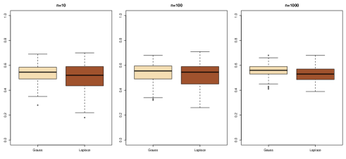
Figure 1: Comparison of the distributions of the posterior probabilities that the data is from a normal model (as opposed to a Laplace model) with unknown mean $\theta$ when the data is made of $n=10,100,1000$ observations (left, centre, right, resp.) either from a Gaussian or Laplace distribution with mean equal to zero and when the summary statistic in the ABC algorithm is the vector made of the collection of the sample mean, median, and variance. The ABC algorithm uses a reference table of $10^{4}$ simulations ($5,000$ for each model) from the prior $\theta\sim\mathcal{N}(0,4)$ and selects the tolerance $\epsilon$ as the $1\%$ distance quantile over those simulations.

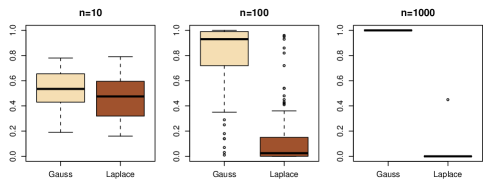
Figure 2: Same legend and same calibration as in Fig. 1 when the ABC algorithm is based on the median absolute deviation of the sample as its sole summary statistic.

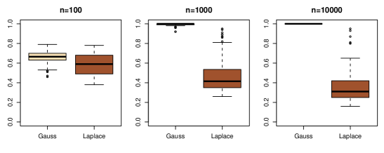
Figure 3: Same legend and same calibration as in Fig. 1, for $n=100,1000,10000$ observations, when the ABC algorithm is based on the empirical fourth moment as its sole summary statistic.

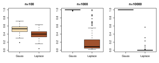
Figure 4: Same legend as in Fig. 3 when the ABC algorithm is based on both the fourth and sixth empirical moments as summary statistics.

The above example illustrates very clearly the major result of this paper, namely that the mean behaviour of the summary statistic $\boldsymbol{T}(\mathbf{y})$ under both models under comparison is fundamental for the convergence of the Bayes factor, i.e. of the Bayesian model choice based on $\boldsymbol{T}(\mathbf{y})$. This result, described in the next section, thus brings an answer to the question raised in Robert et al. (2011) about the validation of ABC model choice, although it may require additional simulation experiments in realistic situations.

The paper is organised as follows: Section 2 contains the theoretical derivation of the asymptotic behaviour of the Bayes factor $B^{\boldsymbol{T}}_{12}(\mathbf{y})$, Section 2.1 covering our main assumptions and exhibiting the asymptotic behaviour of the marginal likelihoods, Section 2.2 detailing the consequences of this result for model choice based on summary statistics. Section 3 illustrates the relevance of our criterion for evaluating summary statistics, including a non-trivial population genetics example. Section 4 details the practical implementation of a validation mechanism based on the above results. Section 5 concludes the paper with a short discussion.

2 Convergence of Bayes factors using summary statistics

Let $\mathbf{y}=(y_{1},\ldots,y_{n})$ be the observed sample, not necessarily iid. We denote by $\mathbf{y}\sim\mathbb{P}^{n}$ the true distribution of the sample, and by $\boldsymbol{T}(\mathbf{y})=\boldsymbol{T}^{n}=(T_{1}(\mathbf{y}),T_{2}(\mathbf{y}),\cdots,T_{d}(\mathbf{y}))$ a $d$-dimensional vector of summary statistics, $\boldsymbol{T}^{n}\sim G_{n}$. The distribution $G_{n}$ is the projection of $\mathbb{P}^{n}$ under the map $\boldsymbol{T}^{n}:\mathbb{R}^{n}\mapsto\mathbb{R}^{d}$ and we denote its density by $g_{n}$.

There are two competing models $\mathfrak{M}_{1}$ and $\mathfrak{M}_{2}$ that we wish to compare:

• under $\mathfrak{M}_{1}$, $\mathbf{y}\sim F_{1,n}(\cdot|\theta_{1})$ where $\theta_{1}\in\Theta_{1}\subset\mathbb{R}^{p_{1}}$,

• under $\mathfrak{M}_{2}$, $\mathbf{y}\sim F_{2,n}(\cdot|\theta_{2})$ where $\theta_{2}\in\Theta_{2}\subset\mathbb{R}^{p_{2}}$.

The distributions of $\boldsymbol{T}^{n}$ under $\mathfrak{M}_{1}$ and $\mathfrak{M}_{2}$ are denoted by $G_{1,n}(\cdot|\theta_{1})$ and $G_{2,n}(\cdot|\theta_{2})$, respectively. We also assume that the distribution functions $F_{i,n}(\cdot|\theta_{i})$, $G_{i,n}(\cdot|\theta_{i})$ have densities $f_{i}(\cdot|\theta_{i})$ and $g_{i}(\cdot|\theta_{i})$ with respect to some dominating measures $(i=1,2)$, respectively. Under the respective prior distributions $\pi_{1}$ and $\pi_{2}$ on $\theta_{1}$ and $\theta_{2}$, the posterior distributions given $\boldsymbol{T}^{n}$ are denoted by $\pi_{1}(\cdot|\boldsymbol{T}^{n})$ and $\pi_{2}(\cdot|\boldsymbol{T}^{n})$.

2.1 Assumptions and asymptotic behaviour of the marginal likelihoods

Before stating the main result in the paper, we detail theoretical assumptions on both the models and the summary statistics under which the main result holds.

We start with a brief primer on our notations. The letter $C$ denotes a generic positive constant (independent of $n$), whose value may change from one occurrence to the next, but is of no consequence. We write $a\wedge b$ to denote $\min(a,b)$. For two sequences $\{a_{n}\},\{b_{n}\}$ of real numbers, $a_{n}\lesssim b_{n}$ (resp. $\gtrsim$) means $a_{n}\leq Cb_{n}$ (resp. $a_{n}\geq Cb_{n})$. Similarly, $a_{n}\sim b_{n}$ means that

$${1/C}\leq\liminf_{n\rightarrow\infty}|a_{n}/b_{n}|\leq\limsup_{n\rightarrow\infty}|a_{n}/b_{n}|\leq C\;.$$

The symbol $\rightsquigarrow$ denotes convergence in distribution.

Technical assumptions that are necessary for establishing the main result of the paper are as follows:

1. There exist a sequence of positive real numbers $\{v_{n}\}$ converging to $+\infty$, a distribution $Q$ on $\mathbb{R}^{d}$, and a vector $\mu_{0}\in\mathbb{R}^{d}$, such that

   $$v_{n}(\boldsymbol{T}^{n}-\mu_{0})\rightsquigarrow Q,\quad\mbox{ under }G_{n}\;.$$

2. For $i\in\{1,2\}$, there exist sieves $\mathcal{F}_{n,i}\subset\Theta_{i}$ and constants $\tau_{i},\alpha_{i},C_{i},x_{0,i}>0$, such that

   $$\pi_{i}(\mathcal{F}_{n,i}^{c})=o(v_{n}^{-\tau_{i}})\,.$$ (2)

   For all $\theta_{i}\in\mathcal{F}_{n,i}$, the asymptotic means $\mu_{i}(\theta_{i})\in\mathbb{R}^{d}$ of $\boldsymbol{T}^{n}$ under this model satisfy: for all $0<x<x_{0,i}v_{n}$

   $$G_{i,n}\Big{[}v_{n}|\boldsymbol{T}^{n}-\mu_{i}(\theta_{i})|>x\,\Big{|}\theta_{i}\Big{]}\leq C_{i}x^{-\alpha_{i}}\,.$$ (3)

   We define the sets $S_{n,i}\subset\mathcal{F}_{n,i}$ $(i=1,2)$ as

   $$S_{n,i}(u)=\big{\{}\theta_{i}\in\mathcal{F}_{n,i};|\mu_{i}(\theta_{i})-\mu_{0}|\leq u\,v_{n}^{-1}\big{\}},\quad u>0\;.$$

We say that $\mathfrak{M}_{i}$ is compatible with $\boldsymbol{T}^{n}$ if

$$\inf\{|\mu_{i}(\theta_{i})-\mu_{0}|;\theta_{i}\in\Theta_{i}\}=0\,,$$

meaning that the asymptotic mean of $\boldsymbol{T}^{n}$ is found within the range of the means of $\boldsymbol{T}^{n}$ in model $\mathfrak{M}_{i}$.

1. If $\mathfrak{M}_{i}$ is compatible with $\boldsymbol{T}^{n}$, then there exists a constant $d_{i}<\tau_{i}\wedge(\alpha_{i}-2)$ such that

   $$\pi_{i}(S_{n,i}(u))\sim u^{d_{i}}v_{n}^{-d_{i}},\quad\forall u\lesssim v_{n}\;.$$ (4)

2. If $\mathfrak{M}_{i}$ is compatible with $\boldsymbol{T}^{n}$, then for any $\epsilon>0$ there exist $U,\delta>0$ and a set $E_{n}$ such that for all $\theta_{i}\in S_{n,i}(U)$

   $$E_{n}\subseteq\{t;g_{i}(t|\theta_{i})\geq\delta g_{n}(t)\}\quad\text{and}\quad G_{n}\left(E_{n}^{c}\right)<\epsilon\,.$$ (5)

Even though these assumptions might appear overwhelming, we claim that (A1)—(A4) are both mild and relatively easy to check in applications. A detailed discussion on those assumptions is provided in Section 2.3. Furthermore, we will later illustrate why they hold in both the Gaussian versus Laplace example (Section 3.1) and a realistic population example (Section 3.3).

The following result provides a fundamental control on the convergence rate of the marginal likelihoods. In Lemma 1, $m_{1}(\cdot)$ and $m_{2}(\cdot)$ denote the marginal densities of $\boldsymbol{T}^{n}$ under models $\mathfrak{M}_{1}$ and $\mathfrak{M}_{2}$, respectively, namely $(i=1,2)$

$$m_{i}(t)=\int_{\Theta_{i}}g_{i}(t|\theta_{i})\,\pi_{i}(\theta_{i})\,\text{d}\theta_{i}\,.$$ (6)

Lemma 1

Under assumptions (A1)–(A4), for $i=1,2$, there exist constants $C_{l},C_{u}=O_{\mathbb{P}^{n}}(1)$ such that, if $\mathfrak{M}_{i}$ is compatible with $\boldsymbol{T}^{n}$, and $\tau_{i}>d_{i}$, $\alpha_{i}>d_{i}+2$,

$$C_{l}v_{n}^{-d_{i}}\leq\frac{m_{i}(\boldsymbol{T}^{n})}{g_{n}(\boldsymbol{T}^{n})}\leq C_{u}v_{n}^{-d_{i}}$$ (7)

and, if $\mathfrak{M}_{i}$ is not compatible with $\boldsymbol{T}^{n}$,

$$\frac{m_{i}(\boldsymbol{T}^{n})}{g_{n}(\boldsymbol{T}^{n})}=O_{\mathbb{P}^{n}}[v_{n}^{-\tau_{i}}+v_{n}^{-\alpha_{i}}].$$ (8)

The above lemma, or more precisely (7), provides an equivalence result for the marginal densities $m_{i}(\boldsymbol{T}^{n})$ when $\mu_{0}\in\{\mu_{i}(\theta_{i}),\theta_{i}\in\Theta_{i}\}$ but it does not specifically require that $G_{n}$ belongs to model $\mathfrak{M}_{i}$. Appendix 2 details the proof of Lemma 1. The following result is a corollary on the use of $\boldsymbol{T}^{n}$ for inference purposes other than model choice:

Corollary 1

Under the assumptions of Lemma 1, if $\mathfrak{M}_{i}$ is compatible with $\boldsymbol{T}^{n}$, the posterior distribution $\pi_{i}(.|\boldsymbol{T}^{n})$ concentrates at the rate $1/v_{n}$ on $\{\theta_{i};\mu_{i}(\theta_{i})=\mu_{0}\}$, provided $\tau_{i}>d_{i}$ and $\alpha_{i}>d_{i}+2$. Hence, under the posterior distribution $\pi_{i}(.|\boldsymbol{T}^{n})$, $\mu_{i}(\theta_{i})$ converges to $\mu_{0}$ at the rate $1/v_{n}$.

Proof 2.1.

Equation (7) of Lemma 1 yields that

$$\frac{m_{i}(\boldsymbol{T}^{n})}{g_{n}(\boldsymbol{T}^{n})}\gtrsim v_{n}^{-d_{i}}\;$$

with large probability. For all sequences $\{w_{n}\}_{n}$ converging to $+\infty$, calculations performed in the proof of Lemma 1 (see Appendix 2) yield that with probability going to 1 under $G_{n}$,

$$\int_{S_{n,i}(w_{n})^{c}}\frac{g_{i}(\boldsymbol{T}^{n}|\theta_{i})}{g_{n}(\boldsymbol{T}^{n})}\,\pi_{i}(\theta_{i})\,\text{d}\theta_{i}\lesssim w_{n}^{-\alpha_{i}}v_{n}^{-\alpha_{i}}+v_{n}^{-\tau_{i}}=o(v_{n}^{-d_{i}})\;.$$

Therefore the posterior distribution of $\mu_{i}(\theta_{i})$ has its tail probability given by

$$\pi_{i}(|\mu_{0}-\mu_{i}(\theta_{i})|>w_{n}v_{n}^{-1}|\boldsymbol{T}^{n})=\frac{\int_{S_{n,i}(w_{n})^{c}}g_{i}(\boldsymbol{T}^{n}|\theta_{i})\pi_{i}(\theta_{i})\,\text{d}\theta_{i}}{m_{i}(\boldsymbol{T}^{n})}=o_{\mathbb{P}^{n}}(1)$$

and the corollary follows. ∎

Lemma 1 helps in understanding the meaning of the parameter $d_{i}$ in assumption (A3) when $\mathfrak{M}_{i}$ is compatible with $\boldsymbol{T}^{n}$. Indeed, we then have

$$\frac{m_{i}(\boldsymbol{T}^{n})}{g_{n}(\boldsymbol{T}^{n})}\sim v_{n}^{-d_{i}}\,,$$

thus $\log(m_{i}(\boldsymbol{T}^{n})/g_{n}(\boldsymbol{T}^{n}))\sim-d_{i}\log v_{n}$ and $v_{n}^{-d_{i}}$ appears as a penalisation factor resulting from integrating $\theta_{i}$ out in the very same spirit as the effective number of parameters appears in the DIC (Spiegelhalter et al., 2002) criterion and in the discussions in Rousseau (2007) and Rousseau and Mengersen (2011). In regular models, $d_{i}$ corresponds to the dimension of $\mu(\Theta_{i})$, leading to the usual BIC approximation; however, in non-regular models, which may occur with the kind of applications where ABC methods are required, $d_{i}$ can be different. This is illustrated in the examples of Section 3. We now present the major implication of these results on the relevance of some summary statistics to compute Bayes factors.

2.2 Bayes factor consistency

Lemma 1 implies that the asymptotic behaviour of the Bayes factor is driven by the asymptotic mean value of $\boldsymbol{T}^{n}$ under both models. It is usual to assume that one of the competing models is true, when studying the behaviour of testing procedures (here posterior probabilities and Bayes factors). Here, in full generality, it is actually enough that one of the models is compatible with the statistic $\boldsymbol{T}^{n}$. Hence, without loss of generality we assume that the true distribution belongs to model $\mathfrak{M}_{1}$ and we first consider the case where model $\mathfrak{M}_{2}$ is also compatible with $\boldsymbol{T}^{n}$, i.e.

$$\inf\{|\mu_{0}-\mu_{2}(\theta_{2})|;\theta_{2}\in\Theta_{2}\}=0\,.$$

Under assumptions (A1)–(A4),

$$C_{l}v_{n}^{-(d_{1}-d_{2})}\leq\dfrac{m_{1}(\boldsymbol{T}^{n})}{m_{2}(\boldsymbol{T}^{n})}\leq C_{u}v_{n}^{-(d_{1}-d_{2})},$$

where $C_{l},C_{u}=O_{\mathbb{P}^{n}}(1)$, irrespective of the true model. Thus the asymptotic behaviour of the Bayes factor depends solely on the difference $d_{1}-d_{2}$. For instance, if $d_{1}>d_{2}$ (as in the embedded case) and $G_{n}$ is in $\mathfrak{M}_{1}$, the Bayes factor goes to 0, instead of infinity. If instead $d_{1}=d_{2}$, the Bayes factor is bounded from below and from above and is thus useless to separate the two models. Note that the asymptotic (non-convergent) behaviour remains the same even when $G_{n}$ is in neither model, provided

$$\inf\{|\mu_{0}-\mu_{2}(\theta_{2})|;\theta_{2}\in\Theta_{2}\}=\inf\{|\mu_{0}-\mu_{1}(\theta_{1})|;\theta_{1}\in\Theta_{1}\}=0\;.$$

On the contrary, assume that the true distribution is in model $\mathfrak{M}_{1}$ and that model $\mathfrak{M}_{2}$ is not compatible with $\boldsymbol{T}^{n}$, then the Bayes factor, under assumptions (A1)–(A4), satisfies

$$\dfrac{m_{1}(\boldsymbol{T}^{n})}{m_{2}(\boldsymbol{T}^{n})}\geq C_{\ell}\min\left(v_{n}^{-(d_{1}-\alpha_{2})},v_{n}^{-(d_{1}-\tau_{2})}\right),$$

and if $\min(\alpha_{2},\tau_{2})>d_{1}$,

$$\lim_{n\rightarrow+\infty}\dfrac{m_{1}(\boldsymbol{T}^{n})}{m_{2}(\boldsymbol{T}^{n})}=+\infty,$$

which leads to choosing the right model asymptotically. The above then implies the following consistency result, which is the core derivation of our paper, providing a characterisation of relevant summary statistics:

Theorem 2.2.

If, under assumptions (A1)–(A4), models $\mathfrak{M}_{1}$ and $\mathfrak{M}_{2}$ are both compatible with $\boldsymbol{T}^{n}$, and $\tau_{i}\wedge\alpha_{i}-2>d_{i}$, then the Bayes factor $B_{12}^{\boldsymbol{T}^{n}}$ has the same asymptotic behaviour as $v_{n}^{-(d_{1}-d_{2})}$, irrespective of the true model. Therefore, it always asymptotically selects the model with the smallest effective dimension $d_{i}$.

If model $\mathfrak{M}_{1}$ is compatible with $\boldsymbol{T}^{n}$ and model $\mathfrak{M}_{2}$ is incompatible with $\boldsymbol{T}^{n}$, then

$$0=\inf\{|\mu_{0}-\mu_{1}(\theta_{1})|;\theta_{1}\in\Theta_{1}\}<\inf\{|\mu_{0}-\mu_{2}(\theta_{2})|;\theta_{2}\in\Theta_{2}\}\,,$$

and if $\min(\alpha_{2},\tau_{2})>d_{1}$, then the Bayes factor $B_{12}^{\boldsymbol{T}}$ is consistent.

Note that, for ancillary statistics, the condition $\min(\alpha_{2},\tau_{2})>d_{1}$ is vacuous since $\tau_{2}=\infty$ and $d_{1}=0$. The theorem therefore also applies to compatible ancillary statistics.

An essential practical consequence of Theorem 2.2 is that the Bayes factor is merely driven by the means $\mu_{i}(\theta_{i})$ and the relative position of $\mu_{0}$ in both sets $\{\mu_{i}(\theta_{i});\theta_{i}\in\Theta_{i}\}$, $i=1,2$. If $G_{n}$ is in neither model but $\mu_{0}$ belongs to $\{\mu_{1}(\theta_{1}),\theta_{1}\in\Theta_{1}\}$ and not to $\{\mu_{2}(\theta_{2}),\theta_{2}\in\Theta_{2}\}$, then the Bayes factor will asymptotically select $\mathfrak{M}_{1}$. Note that the result does not cover the behaviour of the Bayes factor when neither model is compatible with $\boldsymbol{T}^{n}$, since there is no simple characterisation in this case.

The following heuristic argument sheds some light on why the above results hold.

Suppose the summary statistics (appropriately rescaled) are asymptotically normal under each model. Assume that the Kullback-Leibler divergence between the distributions of $\sqrt{n}(\boldsymbol{T}^{n}-\mu_{i}(\theta_{i}))$ can be approximated by the Kullback-Leibler divergence between the respective asymptotic Gaussian distributions

$$\sqrt{n}|V_{0}|^{-1/2}q_{\mathcal{G}}\{\sqrt{n}V_{0}^{-1/2}(\boldsymbol{T}^{n}-\mu_{0})\}$$

and

$$\sqrt{n}|V_{i}(\theta_{i})|^{-1/2}q_{\mathcal{G}}\{\sqrt{n}V_{i}(\theta_{i})^{-1/2}(\boldsymbol{T}^{n}-\mu_{i}(\theta_{i})\}\,,$$

where $V_{0}$, $V_{1}(\theta_{1})$, and $V_{2}(\theta_{2})$ denote the asymptotic variances under the various models, where $|V|$ denotes the determinant of the matrix $V$, and where $q_{\mathcal{G}}$ is the pdf of the standard Gaussian distribution. Then

$$\frac{1}{n}KL\{g_{n}(\boldsymbol{T}^{n}),g_{i}(\boldsymbol{T}^{n}|\theta_{i})\}\approx\frac{(\mu_{0}-\mu_{i}(\theta_{i}))^{t}V_{i}(\theta_{i})^{-1}(\mu_{0}-\mu_{i}(\theta_{i}))}{2}+o(1)\,.$$ (9)

In that case a usual Laplace argument would imply that

$$\frac{m_{i}(\boldsymbol{T}^{n})}{g_{n}(\boldsymbol{T}^{n})}\approx\int\exp\{-\frac{n(\mu_{0}-\mu_{i}(\theta_{i}))^{t}V_{i}(\theta_{i})^{-1}(\mu_{0}-\mu_{i}(\theta_{i}))}{2}\}\,\pi_{i}(\theta_{i})d\theta_{i}.$$

So that the difference between $\mu_{0}$ and $\mu_{i}(\theta_{i})$ is the key measure to evaluate the distance between $g_{n}$ and $g_{i,n}(\cdot|\theta_{i})$. The above argument is purely illustrative since requiring (9) is very strong and not realistic in most cases.

Formally, an ideal statistics $\boldsymbol{T}^{n}$ would be an ancillary statistics for both models with different expectation under both models. Indeed, in this case, the sets $\{\mu_{i}(\theta_{i}),\theta_{i}\in\Theta_{i}\}$ $(i=1,2)$ are singletons and they only have to differ for the Bayes factor to be consistent. For instance, in Example 1, both the empirical variance and the empirical mad statistic are ancillary. In the first case, the expectation is the same under both distribution, which explains why the Bayes factor cannot discriminate between models (Fig. 1). In the second case, the expectations differ, hence a consistent Bayes factor as exhibited in Fig. 2. Concerning the assumptions (A1)–(A4), some simplifications occur under ancillarity:

• assumption (A2) must hold for a single distribution and $\mathcal{F}_{n,i}=S_{n,i}(u)=\Theta_{i}$;

• assumption (A3) holds automatically since $d_{i}=0$;

• assumption (A4) must also hold for the fixed distribution of $\boldsymbol{T}^{n}$ under model $\mathfrak{M}_{i}$ (and obviously holds when $\mathfrak{M}_{i}$ is the true model).

Unfortunately, it is very hard to extract useful ancillary statistics from complex models: while examples of ancillary statistics abound, for instance rank statistics (Sidak et al., 1999), they either do not apply to non-iid settings or have identical means under different models. Example 1 is thus truly a toy example in that it constitutes the exception to this remark. When considering the population genetics models of Section 3, we cannot provide such solutions.

In the special case of $\mathfrak{M}_{1}$ being a submodel of $\mathfrak{M}_{2}$, and if the true distribution belongs to the smaller model $\mathfrak{M}_{1}$, any summary statistic satisfies

$$\mu_{0}\in\{\mu_{1}(\theta_{1});\theta_{1}\in\Theta_{1}\}\subset\{\mu_{2}(\theta_{2});\theta_{2}\in\Theta_{2}\},$$

so that the Bayes factor is of order $v_{n}^{-(d_{1}-d_{2})}$. If the summary statistic is informative merely on a parameter which is the same under both models, i.e., if $d_{1}=d_{2}$, then the Bayes factor is not consistent. Else, $d_{1}<d_{2}$ and the Bayes factor is consistent under $\mathfrak{M}_{1}$. If the true distribution does not belong to $\mathfrak{M}_{1}$, then the same phenomenon as described above occurs and the Bayes factor is consistent only if $\mu_{1}\neq\mu_{2}=\mu_{0}$. This case will be illustrated for a quantile distribution in Section 3.2.

2.3 About the assumptions (A1)–(A4)

Assumptions (A1)–(A4) may appear too stringent or too abstract to be of any practical relevance and we now discuss why they make perfect sense.

Assumption (A1) is quite natural. It is often the case that summary statistics $\boldsymbol{T}^{n}$ are chosen as empirical versions of quantities of interest (under second order moment conditions) and it is natural to assume that they concentrate since they are chosen to be both low dimensional and informative on some aspects of the model (even though the result also applies to ancillary statistics). For instance, when the summary statistics are empirical means or empirical quantiles, (A1) is satisfied with $v_{n}=\sqrt{n}$ and the Gaussian distribution being the limiting $Q$ (a most common occurrence). However, if $\boldsymbol{T}^{n}$ is a distance (e.g., of the type induced by chi-square like statistics) then $Q$ will be the chi-square distribution. We also note that (A1) holds for some ancillary statistics, like those of Example 1.

Assumption (A2) requires that under each model $\boldsymbol{T}^{n}$ concentrates around the model asymptotic mean values $\mu_{i}(\theta_{i})$ at rate $v_{n}$, even though it is not necessary to have convergence in distribution. More precisely, (A2) controls the moderate deviations of the estimator $\boldsymbol{T}^{n}$ from the asymptotic mean $\mu(\theta)$ under each model. For instance, when $\boldsymbol{T}^{n}$ is an empirical mean, i.e., $\boldsymbol{T}^{n}=n^{-1}\sum_{i=1}^{n}h(y_{i})$ for a given function $h$, Markov inequality implies that for every $\theta_{i}\in\Theta_{i}$,

$$G_{i,n}\left[\sqrt{n}|\boldsymbol{T}^{n}-\mu_{i}(\theta_{i})|>u\Big{|}\theta_{i}\right]\leq\frac{\mathbb{E}\Big{[}\left|\sum_{i=1}^{n}\{h(y_{i})-\mu_{i}(\theta_{i})\}\Big{|}\theta_{i}\right|^{p}\Big{]}}{u^{p}\,n^{p/2}}\lesssim u^{-p},$$ (10)

for large values of $p$ (typically, larger than $d_{i}+2$) and under very weak assumptions (much weaker than being in an i.i.d. setting).

Assumption (A3) describes the behaviour of the prior distribution of the mean of $\boldsymbol{T}^{n}$ near the true asymptotic value $\mu_{0}$. This assumption needs only hold on a compatible model and it is often found in the Bayesian asymptotic literature, see for instance condition (2.5) of Theorem 1 in Ghosal and van der Vaart (2007). Usually referred to as the prior mass condition, it corresponds to the fact that if the prior vanishes in regions where the likelihood is not too small (i.e., near $\mu_{0}$ in our case) then the marginal becomes very small. The exponents $d_{i}$ can be viewed as effective dimensions of the parameter under the posterior distributions, as discussed after Corollary 1. If the maps $\theta_{i}\mapsto\mu_{i}(\theta_{i})$ are locally invertible near $\mu_{0}$, under the usual continuity conditions on the maps $\theta_{i}\mapsto|\mu_{0}-\mu_{i}(\theta_{i})|$, for any $u>0$, there exists a finite collection of points $\theta^{*}_{ij}\in\Theta_{i}$ such that the sets $S_{n,i}(u)$ can be bounded both from above and from below by sets of the form

$$\bigcup_{j=1}^{J}\{\theta_{j}:|\theta_{j}-\theta_{ij}^{*}|\lesssim uv_{n}^{-1}\},\quad J\in\mathbb{N}\;.$$ (11)

Thus if the prior density $\pi_{i}$ is bounded from above and below near the points $\theta_{ij}^{*}$, we immediately deduce that $\pi_{i}\{S_{n,i}(u)\}\sim u^{d}v_{n}^{-d}$ and $d_{i}=d$, verifying (A3). In most cases we will have $d_{i}\leq d$, since assuming that $d_{i}>d$ would imply that the prior density of $\mu(\theta)$ explodes at $\mu_{0}$.

Assumption (A4) states that, if there are $\theta_{i}$’s such that $\mu_{i}(\theta_{i})=\mu_{0}$, then uniformly in $\theta$ close to one of those $\theta_{i}$’s, $g_{i}(t|\theta_{i})$ is bounded from below by $\delta g_{n}(t)$ on a set having large probability in terms of $G_{n}$. There are various instances under which this assumption is satisfied. First, if $\mathfrak{M}_{i}$ is the true model and $\boldsymbol{T}^{n}$ is ancillary under this model, it automatically holds since for all $\theta_{i}\in S_{n,i}(u)$ $g_{i}(\cdot|\theta_{i})=g_{n}(\cdot)$. Secondly, if $v_{n}(\boldsymbol{T}^{n}-\mu_{i})$ converges in distribution to $Q$ and if the densities are close, then (A4) is satisfied. This requires in particular that $\boldsymbol{T}^{n}$ has the same support under $G_{n}$ and $G_{i}$, but not necessarily that $G_{i}$ or $G_{n}$ are continuous distributions. Assumption (A4) may become difficult to check when the sets $S_{n,i}(u)$ are not compact, which is typically the case when the sets $\{\theta_{i};\mu_{i}(\theta_{i})=\mu_{0}\}$ are not compact. The important point here is that, in such cases, the posterior distribution $\pi_{i}(\cdot|\boldsymbol{T}^{n})$ is not informative on the whole parameter $\theta_{i}$ (at least no further than the prior) but instead informative on a fraction of it, summarised by $\mu_{i}(\theta_{i})$. Re-parametrising $\theta_{i}$ into $(\mu_{i}(\theta_{i}),\psi_{i})$ where $\psi_{i}$ represents the part of $\theta_{i}$ which is not informed by the asymptotic distribution of $\boldsymbol{T}^{n}$, $\boldsymbol{T}^{n}$ is asymptotically ancillary for $\psi_{i}$. In such a case, (A4) will still hold in situations where the prior distribution does not assign too much mass near the tails, so that the sieves $\mathcal{F}_{n,i}$ can be chosen not too large to ensure that the distributions $G_{i,n}$ of $\boldsymbol{T}^{n}$ hardly depend on $\psi_{i}$.

3 Illustrations

3.1 Gaussian versus Laplace distributions

Recall that in the setting of Example 1, we denote by $\mathfrak{M}_{1}$ the Gaussian model and by $\mathfrak{M}_{2}$ the Laplace model. In each model, the prior on the mean $\theta_{i}$ is a centred Gaussian distribution with variance $4$ and in each case the data are simulated under $\theta_{i}=0$. For illustrating our main result on consistency, we consider the summary statistics made of the empirical fourth moment, $\boldsymbol{T}^{n}=n^{-1}\sum_{i=1}^{n}y_{i}^{4}$, such that $\mu_{1}(\theta)=\theta^{4}+3+6\theta^{2}$ and $\mu_{2}(\theta)=\theta^{4}+6+6\theta^{2}$.

We now endeavour to check that assumptions (A1)–(A4) hold for that statistic. Given that this is an empirical moment, (A1) is trivially satisfied as a consequence of the Central Limit theorem, with $v_{n}=\sqrt{n}$.

For assumption (A2), $\mu_{i}(\theta_{i})$ is already defined above. For both models, we set $\mathcal{F}_{n,1}=\mathcal{F}_{n,2}=\{|\theta|\leq 2\sqrt{\log n}\}=\mathcal{F}_{n}$ for (A2) to hold, so that

$$\pi_{1}(\mathcal{F}_{n,1}^{c})=\pi_{2}(\mathcal{F}_{n,2}^{c})=o(n^{-1})$$

under a Gaussian prior on $\theta$ under both models, which implies $\tau_{i}=2$. The second part of (A2) is verified using Markov inequality. Indeed,

$$\begin{split}G_{i,n}\left[\left.\left|n^{-1}\sum_{j=1}^{n}(y_{j}^{4}-\mu_{i}(\theta))\right|>x\right|\theta\right]&\leq\frac{\mathbb{E}_{i}[(Y^{4}-\mu_{i}(\theta))^{4}|\theta]}{n^{2}x^{4}}\,.\end{split}$$

which implies $\alpha_{i}=4$.

Addressing (A3), in model $\mathfrak{M}_{1}$ if the mean is equal to zero then $\mu_{0}=3$ and, in model $\mathfrak{M}_{2}$ if $\theta_{2}=0$, then $\mu_{0}=6$. Thus $S_{n,1}(u)$ and $S_{n,2}(u)$ can be bounded from above and below by balls of the form

$$|\theta|\leq C\,u^{1/2}n^{-1/4}\,,$$

so that $d_{1}=d_{2}=1/2$ in those cases. Note that, if the mean is different from zero, $\mu_{0}>3$ in model $\mathfrak{M}_{1}$ and $\mu_{0}>6$ in model $\mathfrak{M}_{2}$. Then $S_{n,1}(u)$ and $S_{n,2}(u)$ can be bounded from above and below by balls in the form

$$|\theta^{2}-\theta_{*}^{2}|\leq C\,u\,n^{-1/2},\quad|\theta_{*}|>0$$

so that $d_{1}=d_{2}=1$ in those cases.
Addressing (A4), since both distributions satisfy Cramer condition, the empirical fourth moment allows for an Edgeworth expansion under both models, which can be made uniform in sets in the form $\{|\theta|\leq Cn^{-1/4}\}$, see Bhattacharya and Rao (1986, Theorem 19.1). Hence, (A4) is satisfied.

In conclusion, if the true distribution belongs to model $\mathfrak{M}_{2}$ and the mean is equal to zero, $\mu_{0}\in\{\mu_{i}(\theta);\theta\in\mathbb{R}\}$ for both $i=1,2$ and we have $d_{1}=1$ and $d_{2}=1/2$. On the other hand, if the true distribution belongs to model $\mathfrak{M}_{1}$ then $d_{1}=1/2$ and

$$\inf\{|\mu_{0}-\mu_{2}(\theta_{2})|;\theta_{2}\in\mathbb{R}\}>0\,.$$

Following from Theorem 2.2, the Bayes factor is then consistent but at the rate $n^{-1/4}$ under model $\mathfrak{M}_{2}$. This is to some extent an accidental result, merely due to the fact that, in that very special case when the mean is equal to zero, $d_{1}>d_{2}$. Fig. 3 presented in Section 1.2 illustrates the above discussion. Finally, note that, if the mean is different from zero, then a similar argument leads to the lack of consistency of the Bayes factor, since then $d_{1}=d_{2}=1$ and $\mu_{0}\in\{\mu_{i}(\theta);\theta\in\mathbb{R}\}$, for both $i=1,2$.

3.2 Quantile distributions

We now consider the example of a four-parameter quantile distribution, defined through its quantile function

$$Q(p;A,B,g,k)=A+B\left(1+0.8\frac{1-\exp\{-gz(p)\}}{1+\exp\{-gz(p)\}}\right)\left(1+z(p)^{2}\right)^{k}z(p)$$

where $z(p)$ is the $p$th standard normal quantile and the parameters $A,B,g$ and $k$ represent location, scale, skewness and kurtosis, respectively (Haynes et al., 1997). While the quantile function is well-defined, and the distribution easy to simulate, there is no closed-form expression for the corresponding density function, which makes the implementation of an MCMC algorithm quite delicate. Allingham et al. (2009) introduce a ABC procedure that uses the order statistics as summary statistics. We consider here a model choice perspective.

In this experiment, we set $A=0$ and $B=1$. We then oppose two models:

• model $\mathfrak{M}_{1}$, in which $g=0$, with a single unknown parameter $\theta_{1}=k$ and a prior $\theta_{1}\sim\mathcal{U}[-1/2,5]$. In the simulation process, when $\mathfrak{M}_{1}$ is true, we choose $\theta_{1}=2$.

• model $\mathfrak{M}_{2}$, with two unknown parameters $\theta_{2}=(g,k)$ and a prior $\theta_{2}\sim\mathcal{U}[0,4]\otimes\mathcal{U}[-1/2,5]$. In the simulation process, when $\mathfrak{M}_{2}$ is true, we choose $\theta_{2,1}=1$ and $\theta_{2,2}=2$.

This obviously is a case of embedded models, since $\mathfrak{M}_{1}$ is a sub-model of $\mathfrak{M}_{2}$. As in the previous experiments, we use an ABC procedure relying on $10^{4}$ proposals from the prior and a tolerance set at the $1\%$ quantile of the $L_{1}$ distances between some empirical quantiles. In the comparison below, we first use the empirical quantile of order $10\%$ as sole summary statistic. Then, we consider the empirical quantiles of order $10\%$ and $90\%$, and, at last, the empirical quantiles of order $10\%$, $40\%$, $60\%$ and $90\%$. The results are summarised in Fig. 5. They show complete agreement with Theorem 1.

When the summary statistic $\boldsymbol{T}^{n}$ is restricted to the empirical quantile of order $10\%$, the Bayes factor is not consistent. Indeed, in such a case, we have

$$\mu_{1}(\theta_{1})=\left(1+z(0.1)^{2}\right)^{\theta_{1}}z(0.1)\,,$$

and

$$\mu_{2}(\theta_{2})=\left(1+0.8\frac{1-\exp(-\theta_{2,1}z(0.1))}{1+\exp(-\theta_{2,1}z(0.1))}\right)\left(1+z(0.1)^{2}\right)^{\theta_{2,2}}z(0.1)\,.$$

When $\mathfrak{M}_{1}$ is true with $k=2$, then $\mu_{0}\approx-8.95$ and $\inf\{|\mu_{0}-\mu_{1}(\theta_{1})|;\theta_{1}\in\Theta_{1}\}=\inf\{|\mu_{0}-\mu_{2}(\theta_{2})|;\theta_{2}\in\Theta_{2}\}=0$. Similarly, when $\mathfrak{M}_{2}$ is true with $g=1$ and $k=2$, then $\mu_{0}\approx-4.90$ and

$$\inf\{|\mu_{0}-\mu_{1}(\theta_{1})|;\theta_{1}\in\Theta_{1}\}=\inf\{|\mu_{0}-\mu_{2}(\theta_{2})|;\theta_{2}\in\Theta_{2}\}=0\,.$$

Therefore, the Bayes factor has the same asymptotic behaviour as $n^{-(d_{1}-d_{2})/2}$, irrespective of the true model. We can prove that $d_{1}=d_{2}=1$ in this case, therefore that the Bayes factor is not consistent.

When the summary statistics $\boldsymbol{T}^{n}$ is the vector made of the empirical quantiles of order $10\%$ and $90\%$, the Bayes factor is consistent. Indeed, in such a case, we have

$$\mu_{1}(\theta_{1})=\left[\left(1+z(0.1)^{2}\right)^{\theta_{1}}z(0.1),\left(1+z(0.9)^{2}\right)^{\theta_{1}}z(0.9)\right]\,,$$

and

$$\mu_{2}(\theta_{2})=\left[\left(1+0.8\frac{1-\exp(-\theta_{2,1}z(0.1))}{1+\exp(-\theta_{2,1}z(0.1))}\right)\left(1+z(0.1)^{2}\right)^{\theta_{2,2}}z(0.1),\right.$$

$$\left.\left(1+0.8\frac{1-\exp(-\theta_{2,1}z(0.9))}{1+\exp(-\theta_{2,1}z(0.9))}\right)\left(1+z(0.9)^{2}\right)^{\theta_{2,2}}z(0.9)\right]\,.$$

When $\mathfrak{M}_{1}$ is true with $k=2$, then $\mu_{0}\approx[-8.95,8.95]$ and

$$\inf\{|\mu_{0}-\mu_{1}(\theta_{1})|;\theta_{1}\in\Theta_{1}\}=\inf\{|\mu_{0}-\mu_{2}(\theta_{2})|;\theta_{2}\in\Theta_{2}\}=0\,.$$

We can prove that $d_{1}<d_{2}$ and hence that the Bayes factor is consistent. Moreover, when $\mathfrak{M}_{2}$ is true with $g=1$ and $k=2$, then $\mu_{0}\approx[-4.90,12.99]$, and

$$\inf\{|\mu_{0}-\mu_{2}(\theta_{2})|;\theta_{2}\in\Theta_{2}\}=0\quad\text{ but }\quad\inf\{|\mu_{0}-\mu_{2}(\theta_{1})|;\theta_{1}\in\Theta_{1}\}>0\,.$$

We can prove that $\min(\alpha_{1},\tau_{1})>d_{2}$ and therefore that the Bayes factor is again consistent.

Finally, when the summary statistics $\boldsymbol{T}^{n}$ is the larger vector made of the empirical quantiles of order $10\%$, $40\%$, $60\%$ and $90\%$, the Bayes factor is obviously consistent. However, the results obtained in Fig. 5 are very similar to the ones obtained with only two empirical quantiles.

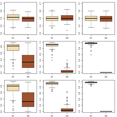
Figure 5: Comparison of the distributions of the posterior probabilities that the quantile distribution data is from model $\mathfrak{M}_{1}$ when the data is made of 100 observations (left column), 1000 observations (central column) and 10,000 observations (right column) either from $\mathfrak{M}_{1}$ (M1) or $\mathfrak{M}_{2}$ (M2) when the summary statistics in the ABC algorithm are made of the empirical quantile at level $10\%$ (first row), the empirical quantiles at levels $10\%$ and $90\%$ (second row), and the empirical quantiles at levels $10\%$, $40\%$, $60\%$ and $90\%$ (third row), respectively. The boxplots rely on $100$ replicas and the ABC algorithms are based on $10^{4}$ proposals ($5,000$ for each model) from the prior, with the tolerance being chosen as the $1\%$ quantile on the distances.

3.3 Population genetics experiment

We now examine a Monte Carlo experiment that more directly relates to the genesis of ABC, namely population genetics. As in Robert et al. (2011), we consider two populations (1 and 2) having diverged at a fixed time $t^{\prime}$ in the past and a third population (3) having diverged from one of those two populations (models 1 and 2, respectively). Times are set to $t^{\prime}=60$ generations for the first divergence and $t=30$ generations for the second one. The effective population size is assumed to be identical for all three populations and equal to $N_{e}=60$. Recall that the effective size of a population is defined as the size of an ideal (Wright-Fisher) population that would show the same behaviour as the population of interest, in terms of loss of genetic variation due to random drift.
We assume we observed 50 diploid individuals per population genotyped at 5, 50 or 100 independent microsatellite loci, this number acting as a proxy to the sample size. These loci are assumed to evolve according to the stepwise mutation model: when a mutation occurs, the number of repetitions of the mutated gene increases or decreases by one unit with equal probability. For each configuration (defined in terms of loci numbers), we generate 100 observations for which the mutation rate $\theta$ is common to all loci and set to $0.005$. In these experiments, both scenarios have a single parameter, the mutation rate $\theta$. We chose a uniform prior distribution $\mathcal{U}[0.0001,0.01]$ on this parameter $\theta$.

For the ABC analysis, we use three summary statistics associated to the $(\delta\mu)^{2}$ distances (Goldstein et al., 1995, Cooper et al., 1999). Let $x_{l,i,j}$ be the repeated number of allele in locus $l=1,\ldots,n$ ($n=5,50,100$) for individual $i=1,\dots,100$ (corresponding to $50$ diploid individuals) within population $j=1,2,3$. The $(\delta\mu)^{2}$ distance between population $j_{1}$ and $j_{2}$, denoted by $(\delta\mu)^{2}_{j_{1},j_{2}}$, is:

$$(\delta\mu)^{2}_{j_{1},j_{2}}=\frac{1}{n}\sum_{l=1}^{n}\left(\frac{1}{100}\sum_{i_{1}=1}^{100}x_{l,i_{1},j_{1}}-\frac{1}{100}\sum_{i_{2}=1}^{100}x_{l,i_{2},j_{2}}\right)^{2}\,.$$

Let us consider two copies of the locus $l$ with allele sizes $x_{l,i,j_{1}}$ and $x_{l,i^{\prime},j_{2}}$, and assume that the most recent time in the past for which they have a common ancestor, defined as the coalescence time $\tau_{j_{1},j_{2}}$, is known. The two copies are then separated by a branch of gene genealogy of total length $2\tau_{j_{1},j_{2}}$. As explained in Slatkin (1995), according to the coalescent process, during that time the number of mutations is a random variable distributed from a Poisson distribution with parameter $2\mu\tau_{j_{1},j_{2}}$. Therefore, if the stepwise mutation model is adopted, we get (under models 1 and 2)

$$\mathbb{E}^{i}\left\{\left(x_{l,i,j_{1}}-x_{l,i^{\prime},j_{2}}\right)^{2}|\tau_{j_{1},j_{2}}\right\}=2\theta\tau_{j_{1},j_{2}}\,.$$

In addition, if $j_{1}=1$ and $j_{2}=2$, we have (under models 1 and 2)

$$\mathbb{E}\left\{\tau_{1,2}\right\}=\left(2N_{e}+t^{\prime}\right)\,,$$

and

$$\mathbb{E}\left\{\left(x_{l,i,1}-x_{l,i^{\prime},2}\right)^{2}\right\}=4N_{e}\theta+2\theta t^{\prime}\,.$$

Moreover,

$$\left(x_{l,i,1}-x_{l,i^{\prime},2}\right)^{2} =\left(x_{l,i,1}-\frac{1}{100}\sum_{i_{1}=1}^{100}x_{l,i_{1},1}+\frac{1}{100}\sum_{i_{1}=1}^{100}x_{l,i_{1},1}\right.$$

$$\left.+\frac{1}{100}\sum_{i_{2}=1}^{100}x_{l,i_{2},2}-\frac{1}{100}\sum_{i_{2}=1}^{100}x_{l,i_{2},2}-x_{l,i^{\prime},2}\right)^{2}$$

And

$$\mathbb{E}\left\{\left(x_{l,i,1}-\frac{1}{100}\sum_{i_{1}=1}^{100}x_{l,i_{1},1}\right)^{2}\right\}+\mathbb{E}\left\{\left(x_{l,i^{\prime},2}-\frac{1}{100}\sum_{i_{2}=1}^{100}x_{l,i_{2},2}\right)^{2}\right\}+$$

$$\quad\mathbb{E}\left\{\left(\frac{1}{100}\sum_{i_{1}=1}^{100}x_{l,i_{1},1}-\frac{1}{100}\sum_{i_{2}=1}^{100}x_{l,i_{2},2}\right)^{2}\right\}=4N_{e}\theta+2\theta t^{\prime}\,.$$

The coalescent process associated to the stepwise mutation model gives

$$\mathbb{E}\left\{\left(x_{l,i,1}-\frac{1}{100}\sum_{i_{1}=1}^{100}x_{l,i_{1},1}\right)^{2}\right\}=\mathbb{E}\left\{\left(x_{l,i^{\prime},2}-\frac{1}{100}\sum_{i_{2}=1}^{100}x_{l,i_{2},2}\right)^{2}\right\}=2N_{e}\theta\,,$$

and then

$$\mathbb{E}\left\{(\delta\mu)^{2}_{1,2}\right\}=2\theta t^{\prime}\,.$$

We can apply the same type of reasoning to the other $(\delta\mu)^{2}$ distances, and if $\mu_{i}$ denotes the mutation rate under model $i$, we get the results given in Table 1.

Table 1: Theoretical expectations of the $(\delta\mu)^{2}_{a,b}$ statistics under both models

	Model 1	Model 2
$\mathbb{E}\left\{(\delta\mu)^{2}_{1,2}\right\}$	$2\theta_{1}t^{\prime}$	$2\theta_{2}t^{\prime}$
$\mathbb{E}\left\{(\delta\mu)^{2}_{1,3}\right\}$	$2\theta_{1}t$	$2\theta_{2}t^{\prime}$
$\mathbb{E}\left\{(\delta\mu)^{2}_{2,3}\right\}$	$2\theta_{1}t^{\prime}$	$2\theta_{2}t$

Given the complexity of this genetic model, it provides a realistic example of relevant statistics satisfying the assumptions (A1)–(A4). Let us consider the associated statistics $(\delta\mu)^{2}_{1,2}$. This is an empirical mean of variables

$$Y_{l}=\left(\frac{1}{100}\sum_{i_{1}=1}^{100}x_{l,i_{1},1}-\frac{1}{100}\sum_{i_{2}=1}^{100}x_{l,i_{2},2}\right)^{2}\,,$$

which are independent and identically distributed. Moreover, since for each couple $(i_{1},i_{2})$, $\left(x_{l,i_{1},1}-x_{l,i_{2},2}\right)$ is bounded by a Poisson random variable, then, under each model, $Y_{l}$ has moments of all orders and $(100)^{2}Y_{l}\in\mathbb{Z}$. Thus, using Theorem 2.2.1 of Bhattacharya and Rao (1986), we obtain that for all $s\geq 2$ and all $\theta_{i}$

$$(1+|t|^{s})\left|g_{i}(t|\theta_{i})-p_{n,s,\theta_{i}}(n^{1/2}(t-\mu_{i}(\theta_{i})))\right|=o(n^{(s-1)/2})$$ (12)

where

1. the order $o(n^{(s-1)/2})$ is uniform over $t\in\mathbb{Z}/(100^{2}n)$ and over compact subsets of $\Theta_{i}\subset\mathbb{R}^{+}$,

2. $p_{n,s,\theta_{i}}(n^{1/2}(t-\mu_{i}(\theta_{i})))$ is the Edgeworth expansion of the density of $(\delta\mu)^{2}_{1,2}$:

   $$p_{n,s,\theta_{i}}(n^{1/2}\{t-\mu_{i}(\theta_{i})\})=n^{-1/2}\phi(n^{1/2}(t-\mu_{i}(\theta_{i}))/\sigma_{i}(\theta_{i}))+o(n^{-1/2})$$

   for some $\sigma_{i}(\theta_{i})>0$.

If under the true distribution $Y_{l}$ also has at least $s\geq 2$ moments, then

$$g_{n}(t)=n^{-1/2}\phi(n^{1/2}(t-\mu_{0})/\sigma_{0})+o(n^{-1/2}),\quad\forall t\in\mathbb{Z}/(100^{2}n)$$ (13)

for some $\mu_{0}\in\mathbb{R}$ and $\sqrt{n}((\delta\mu)^{2}_{1,2}-\mu_{0})\rightsquigarrow\mathcal{N}(0,\sigma_{0}^{2})$ thus (A1) is satisfied with $v_{n}=\sqrt{n}$. Introducing $E_{n}=\{t\in\mathbb{Z}/(100^{2}n);|t-\mu_{0}|\leq n^{-1/2}\gamma_{\epsilon}\}$, $G_{n}(E_{n}^{c})<\epsilon$ from (13) and (12) implies that, if $|\mu_{i}(\theta_{i})-\mu_{0}|\leq\delta_{0}n^{-1/2}$, $g_{i}(t|\theta_{i})\geq\delta g_{n}(t)$ for all $t\in E_{n}$ by choosing $\delta_{0}$ small enough. Hence (A4) is verified. Moreover, if model $\mathfrak{M}_{i}$ is compatible, $\mu_{1}(\theta_{1})=2\theta_{1}t^{\prime}$ and $\mu_{2}(\theta_{2})=2\theta_{2}t^{\prime}$, for $\mu_{0}\in(0.0002t^{\prime},0.02t^{\prime})$,

$$\pi_{i}\left(S_{n,i}(u)\right)\sim u\,n^{-1/2}$$

and (A3) is satisfied with $d_{i}=1$. It is straightforward to verify (A2). Indeed, if model $\mathfrak{M}_{i}$ is not compatible, choosing $\epsilon_{i}>\inf\{|\mu_{0}-\mu_{i}(\theta_{i})|;\theta_{i}\in(0.0001,0.01)\}$, for all $\theta_{i}\in(0.0001,0.01)$, using (12) we get

$$G_{i,n}[|(\delta\mu)^{2}_{1,2}-\mu_{i}(\theta_{i})|>\epsilon_{i}|\theta_{i}]=o(n^{-(s-1)/2})$$

uniformly in $\theta_{i}$ for all $s\geq 2$. If model $\mathfrak{M}_{i}$ is compatible, using Markov inequality,

$$G_{i,n}[|(\delta\mu)^{2}_{1,2}-\mu_{i}(\theta_{i})|>x|\theta_{i}]\leq\frac{\mathbb{E}_{\theta_{i}}\left[|(\delta\mu)^{2}_{1,2}-\mu_{i}(\theta_{i})|^{4}\right]}{x^{4}}$$ (14)

and (A2) is satisfied with $\alpha_{i}=4$. We can use the same arguments to show that assumptions (A1)–(A4) holds also if $\boldsymbol{T}^{n}(\mathbf{y})=((\delta\mu)^{2}_{1,3},(\delta\mu)^{2}_{2,3})$.

Table 1 indicates that whatever model the data originates from (whether $\mathfrak{M}_{1}$ or $\mathfrak{M}_{2}$), the Bayes factor based only on the distance $(\delta\mu)^{2}_{1,2}$ as the summary statistic does not converge. Indeed, if $\theta_{1}=\theta_{2}$, we get the same expectation on the first line of Table 1. The same occurs when only $(\delta\mu)^{2}_{1,3}$ (resp. $(\delta\mu)^{2}_{2,3}$) is used. Indeed, in that case, if $\theta_{1}=2\theta_{2}$ (resp. $2\theta_{1}=\theta_{2}$) we get the same expectation on the second (resp., the third) row of Table 1. Now, if either two or three of the distances are used, the Bayes factors do converge. Indeed, in these settings, no value of $\theta_{1}$ and $\theta_{2}$ can produce equal expectations.

Fig. 6 shows how the empirical results confirm this theoretical analysis. Even the medium case of 50 loci indicates whether the use of the corresponding summary statistic(s) is valid or not. Under both models, the ABC computations have been performed using the DIY-ABC software (Cornuet et al., 2008).

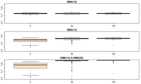
Figure 6: Comparison of the distributions of the posterior probabilities that the data is from model 1 for 5, 50 and 100 loci (left, centre, right, resp.) when the summary statistic in the ABC algorithm is made of different $(\delta\mu)^{2}$ distances. The ABC algorithm uses $2\times 10^{5}$ proposals ($10^{5}$ for each model) from the prior and selects the tolerance $\epsilon$ as the $0.5\%$ distance quantile.

4 Checking for relevant statistics

4.1 A practical procedure

While Theorem 1 operates in an asymptotic and theoretical framework, it is nonetheless possible to find a methodological consequence from this characterisation of consistent summary statistics for testing. This result states that the summary statistic $\boldsymbol{T}^{n}$ is not consistent (and thus unacceptable) for testing between models when both models are compatible with $\boldsymbol{T}^{n}$, in other words when

$$\inf\{|\mu_{1}(\theta_{1})-\mu_{0}|;\theta_{1}\in\Theta_{1}\}=\inf\{|\mu_{2}(\theta_{2})-\mu_{0}|;\theta_{2}\in\Theta_{2}\}=0\,.$$

Based on this our asymptotic result, we propose to run a practical check of the relevance (or non-relevance) of $\boldsymbol{T}^{n}$. The null hypothesis of this test is expressed as both models are compatible with the statistic $\boldsymbol{T}^{n}$. The testing procedure then provides estimates of the mean of $\boldsymbol{T}^{n}$ under each model and checks whether or not those means are equal. For the sake of clarity, we assume without loss of generality that $\mathfrak{M}_{1}$ is the true model (recall that it is enough to have this model compatible with the statistic $\boldsymbol{T}^{n}$), so checking the relevance of $\boldsymbol{T}^{n}$ means testing for

$$H_{0}:\inf\{|\mu_{2}(\theta_{2})-\mu_{0}|;\theta_{2}\in\Theta_{2}\}=0$$

against

$$H_{1}:\inf\{|\mu_{2}(\theta_{2})-\mu_{0}|;\theta_{2}\in\Theta_{2}\}>0.$$

Corollary 1 implies that, when model $\mathfrak{M}_{i}$ is compatible with $\boldsymbol{T}^{n}$, the predictive value of the summary statistic, $\mathbb{E}^{\pi}\left[\boldsymbol{T}^{n}(\mathbf{y}^{\rm{new}})|\boldsymbol{T}^{n}(\mathbf{y})\right]$, is approximately equal to $\mu_{0}$ ($\mathbf{y}$ denotes the observed summary statistic):

$$\begin{split}\mathbb{E}^{\pi}\left[\boldsymbol{T}^{n}(\mathbf{y}^{\rm{new}})|\boldsymbol{T}^{n},\mathfrak{M}_{i}\right]&=\int tg_{i,n}(t|\theta_{i})dtd\pi_{i}(\theta_{i}|\boldsymbol{T}^{n}(\mathbf{y}))\\ &=\int_{\Theta_{i}}\mu_{i}(\theta_{i})d\pi_{i}(\theta_{i}|\boldsymbol{T}^{n}(\mathbf{y}))\\ &=\mu_{0}+\int_{\Theta_{i}}(\mu_{i}(\theta_{i})-\mu_{0})d\pi_{i}(\theta_{i}|\boldsymbol{T}^{n}(\mathbf{y}))\,.\end{split}$$

When $|\mu_{i}(\theta_{i})|$ is bounded on $\Theta_{i}$ (for instance when $\Theta_{i}$ is compact and $\mu_{i}(\cdot)$ is continuous)

$$\int_{\Theta_{i}}(\mu_{i}(\theta_{i})-\mu_{0})d\pi_{i}(\theta_{i}|\boldsymbol{T}^{n}(\mathbf{y}))=o_{p}(1).$$

Thus, under the null (non-relevance of $\boldsymbol{T}^{n}$), we have

$$\mathbb{E}^{\pi}\left[\boldsymbol{T}^{n}(\mathbf{y}^{\rm{new}})|\boldsymbol{T}^{n}(\mathbf{y}),\mathfrak{M}_{1}\right]=\mathbb{E}^{\pi}\left[\boldsymbol{T}^{n}(\mathbf{y}^{\rm{new}})|\boldsymbol{T}^{n}(\mathbf{y}),\mathfrak{M}_{2}\right]+o_{p}(1)=\mu_{0}+o_{p}(1)$$

and the proximity of both predictive values indicates that the statistic $\boldsymbol{T}^{n}$ is not discriminant.

To quantify what this notion of proximity means we advocate using the following practical procedure. Under each model $\mathfrak{M}_{i}$, $i=1,2$, run an ABC sample producing a sample $\theta_{i,l},l=1,\cdots,L$ from the approximate posterior distribution of $\theta_{i}$ given $\boldsymbol{T}^{n}(\mathbf{y})$. Note that $L$ can be chosen to be arbitrarily large. For each value $\theta_{i,l}$, generate $\mathbf{y}_{i,l}\sim F_{i,n}(\cdot|\psi_{i,l})$, derive $\boldsymbol{T}^{n}(\mathbf{y}_{i,l})$ and compute

$$\hat{\mu_{i}}=\frac{1}{L}\sum_{l=1}^{L}\boldsymbol{T}^{n}(\mathbf{y}_{i,l}),\quad i=1,2\,.$$

Conditionally on $\boldsymbol{T}^{n}(\mathbf{y})$, we have

$$\sqrt{L}(\hat{\mu_{i}}-\mathbb{E}^{\pi}\left[\mu_{i}(\theta_{i})|\boldsymbol{T}^{n}(\mathbf{y})\right])\rightsquigarrow\mathcal{N}(0,V_{i}),$$

for some $V_{i}$, as $L$ goes to infinity. Therefore, we propose to test for a common mean

$$H_{0}:\hat{\mu_{1}}\sim\mathcal{N}(\mu_{0},V_{1})\,,\hat{\mu_{2}}\sim\mathcal{N}(\mu_{0},V_{2})$$

against the alternative of different means

$$H_{1}:\hat{\mu_{i}}\sim\mathcal{N}(\mu_{i},V_{i}),\quad\mbox{ with }\mu_{1}\neq\mu_{2}\,.$$

This test is implemented using the fact that asymptotically the decision statistic

$$(\hat{\mu}_{1}-\hat{\mu}_{2})^{\text{T}}(V_{1}+V_{2})^{-1}(\hat{\mu}_{1}-\hat{\mu}_{2})$$

converges to a chi-squared distribution even in the case the covariance matrices $V_{1}$ and $V2$ are estimated by convergent estimators, e.g. empirical covariances. If the null hypothesis $H_{0}$ cannot be rejected, we conclude that the statistic $\boldsymbol{T}^{n}(\mathbf{y})$ is not adequate for model choice.

4.2 Gaussian versus Laplace distributions

In the case of the normal versus Laplace toy problem, we ran a hundred evaluations based on three and four statistics, i.e. the empirical mean, median and variance, without and with the empirical mad. The two choices of the summary statistic vector led to two different ABC approximations of the posterior distribution. Under each model, the ABC procedure is based on a fixed reference table of $5\times 10^{4}$ proposals from the prior $\theta\sim\mathcal{N}(0,4)$ and the respective model, and it selects the tolerance $\epsilon$ as the $1\%$ quantile of the deduced simulation distances. Then, under each model, we get a $500$-sample as an approximation of the posterior distributions. For each of those values, we simulated samples from the models, with the same size as the original sample, producing samples $\boldsymbol{T}^{n}(\mathbf{y}_{i,l})$, and we derived from those samples $\chi^{2}$ tests about the equality of the means. Fig. 7 evaluates the impact of including the empirical mad within those summary statistics on the result of the $\chi^{2}$ test. The result of this simulation experiment (based on 100 replications) is quite satisfactory in that in approximately $95\%$ of cases the difference between the two empirical means falls within the null hypothesis acceptance interval associated with a $5\%$ error when the empirical mad is not included, therefore concluding on the inappropriateness of the summary statistics to conduct the ABC model comparison. On the opposite, the difference always is outside the null hypothesis acceptance interval when the empirical mad is included.

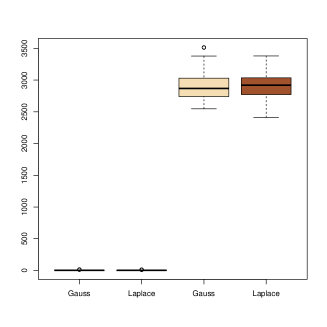
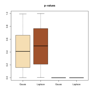
Figure 7: Boxplot representation of the variability of the test statistics (left) and corresponding p-values (right) comparing the expectation of two vectors of summary statistics: the empirical mean, median and variance (left block within each graph) and the previous three ones plus the empirical mad (right block within each graph).

4.3 Population genetics experiment

For the population genetics example, we ran a comparison experiment between the case when we use $(\delta\mu)^{2}_{1,2}$ as sole summary statistic and when we use instead the vector $\left((\delta\mu)^{2}_{1,3},(\delta\mu)^{2}_{2,3}\right)$. The results are presented in Fig. 8. For each of the $100$ points used for the boxplots, the data is made of $n=100$ loci and the $t$-statistics are based on $500$ samples under each model. In fact, the ABC algorithm relies on a fixed reference table of $10^{5}$ proposals from the prior and the respective model, and it selects the tolerance $\epsilon$ as the $0.5\%$ quantile of the deduced simulation distances. As for the previous example, the result of this simulation experiment is quite satisfactory. It highlights the ability of our empirical procedure to detect inappropriate summary statistics. We can truly compare the expectation of a summary statistics under both models using parameter values drawn from the ABC posterior approximation.

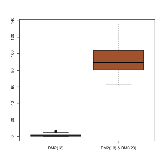
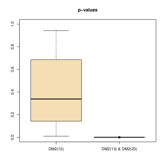
Figure 8: Boxplot representation of the variability of the test statistics (left) and corresponding p-values (right) comparing the mean of the summary statistics $(\delta\mu)^{2}_{1,2}$ and $\left((\delta\mu)^{2}_{1,3},(\delta\mu)^{2}_{2,3}\right)$.

5 Discussion

This paper has produced sufficient conditions for a summary statistics to produce a consistent or an inconsistent Bayesian model choice. It thus brings an answer to the question raised in Robert et al. (2011), which was warning the ABC community about the potential pitfalls of an uncontrolled use of ABC approximations to Bayes factors. The central condition that the true asymptotic mean of the summary statistic should not be recovered under the wrong model if model choice is to take place (in a convergent manner) is both natural, in that the asymptotic normality implies that only first moments matter, and fundamental, in that it drives the choice of summary statistics in practical settings, first and foremost for the ABC algorithm. Indeed, Theorem 2.2 implies that estimation statistics should not be used in ABC algorithms aiming at model comparison, unless their expectation can be shown to differ under both models. This means that (a) different statistics should be used for estimation and for testing and (b) that they should not be mixed in a single summary statistic. Note that the distinction differs from the sufficient versus ancillary opposition found in classical statistics (Cox and Hinkley, 1994) in that it is enough that the summary statistic $\boldsymbol{T}^{n}$ has a different asymptotic mean under both models. In addition, and as shown in the normal-Laplace example in Section 3.1, some ancillary statistics may not be appropriate for testing.

At a methodological level, the classification of summary statistics resulting from the present study is paramount: when comparing models with a given range of potential summary statistics, the expectations of the various summary statistics can be evaluated by simulation under all models. For instance, in ABC settings, the production of pseudo-data is a requirement for the implementation of the method; it is therefore quite straightforward to test via a preliminary experiment whether the condition of Theorem 2.2 holds.

Neither the final choice of summary statistics as in Fearnhead and Prangle (2012), nor the comparison with alternative model comparisons techniques such as $\text{ABC}_{\mu}$ (Ratmann et al., 2009) are covered in the current paper. These obviously are issues worth investigating and they constitute seeds for future development in the area.

Appendix 1

Proof of Lemma 1

Recall that $G_{n}$ is the true distribution of $\boldsymbol{T}^{n}$. Let us first assume that $\inf\{|\mu_{0}-\mu_{i}(\theta_{i})|;\theta_{i}\in\Theta_{i}\}=0$ and let $S_{n,i}$ be defined as in (A3). Note that from (A1), for all $\delta>0$, there exists $M_{\delta}>0$ such that for $n$ large enough

$$G_{n}(|\boldsymbol{T}^{n}-\mu_{0}|>M_{\delta}/v_{n})<\delta.$$ (15)

and note that $M_{\delta}$ goes to infinity as $\delta$ goes to 0. Let $\epsilon>0$ and consider the set $E_{n}$, and the positive constants $U_{\epsilon}$ and $\delta_{\epsilon}$ defined in (A4). From (6) we have for all $\boldsymbol{T}^{n}\in E_{n}$,

$$\begin{split}m_{i}(\boldsymbol{T}^{n})&\geq\int_{S_{n,i}(U_{\epsilon})}g_{i}(\boldsymbol{T}^{n}|\theta_{i})\,\pi_{i}(\theta_{i})\,\text{d}\theta_{i}\,\\ &\geq\delta_{\epsilon}g_{n}(\boldsymbol{T}^{n})\pi_{i}(S_{n,i}(U_{\epsilon}))\geq c_{\epsilon}g_{n}(\boldsymbol{T}^{n})v_{n}^{-d_{i}}\end{split}$$

for some positive constant $c_{\epsilon}$, where the second inequality follows from the definition of $E_{n}$ and the last from (A3). Formally, since $G_{n}(E_{n})\geq 1-\epsilon$, there exists $c_{\epsilon}>0$ such that for $n$ large enough

$$G_{n}\left[m_{i}(\boldsymbol{T}^{n})\geq c_{\epsilon}\,g_{n}(\boldsymbol{T}^{n})v_{n}^{-d_{i}}\right]\geq 1-\epsilon.$$ (16)

We now obtain an upper bound for $m_{i}(\boldsymbol{T}^{n})$. Using (6) we write,

$$m_{i}(\boldsymbol{T}^{n}) = \int_{\mathcal{F}_{n,i}}g_{i}(\boldsymbol{T}^{n}|\theta_{i})\,\pi_{i}(\theta_{i})\,d\theta_{i}+\int_{\mathcal{F}_{n,i}^{c}}g_{i}(\boldsymbol{T}^{n}|\theta_{i})\,\pi_{i}(\theta_{i})\,d\theta_{i}\;.$$

As before fix $\delta>0$ and let $M_{\delta}$ be defined as in (15). Applying Markov inequality and Fubini’s theorem, we obtain that, for all $\epsilon>0$,

$$\begin{split}&G_{n}\Big{(}\int_{\mathcal{F}_{n,i}^{c}}g_{i}(\boldsymbol{T}^{n}|\theta_{i})\,\pi_{i}(\theta_{i})\,d\theta_{i}>\epsilon\,g_{n}(\boldsymbol{T}^{n})\,\pi_{i}(S_{n,i})\Big{)}\\ &\leq G_{n}[|\boldsymbol{T}^{n}-\mu_{0}|>M_{\delta}v_{n}^{-1}]\\ &+\int_{\mathcal{F}_{n,i}^{c}}\int_{v_{n}|t-\mu_{0}|\leq M_{\delta}}\frac{1}{\epsilon\,g_{n}(t)\,\pi_{i}(S_{n,i})}g_{n}(t)g_{i}(t|\theta_{i})dt\,\pi_{i}(\theta_{i})\,d\theta_{i}\\ &\leq G_{n}[|\boldsymbol{T}^{n}-\mu_{0}|>M_{\delta}v_{n}^{-1}]\\ &+\int_{\mathcal{F}_{n,i}^{c}}\frac{1}{\epsilon\,\pi_{i}(S_{n,i})}\int_{\mathbb{R}^{d}}g_{i}(t|\theta_{i})dt\,\pi_{i}(\theta_{i})\,d\theta_{i}\\ &\leq\delta+\frac{\pi(\mathcal{F}_{n,i}^{c})}{\epsilon\pi_{i}(S_{n,i})}\leq 2\delta,\end{split}$$ (17)

given the conditions imposed by (A2) and (A3), when $n$ is large enough.

We can represent $\mathcal{F}_{n,i}$ as a finite disjoint union of the following sets:

$$\mathcal{F}_{n,i} = \bigcup_{j=0}^{J_{n}+1}\mathcal{H}_{j},\quad J_{n}=J_{0}v_{n},\quad\mathrm{for}\,\,\mathrm{some}\,\,J_{0}\in\mathbb{N}\,,$$

$$\mathcal{H}_{j} = S_{n,i}((j+1)M_{\delta})\cap S_{n,i}(jM_{\delta})^{c},\quad j\leq J_{n}\,,$$

$$\mathcal{H}_{J_{n}+1} = \mathcal{F}_{n,i}\cap S_{n,i}^{c}(M_{\delta}J_{n})\;.$$

Now we have

$$\int_{\mathcal{F}_{n,i}}g_{i}(\boldsymbol{T}^{n}|\theta_{i})\,\pi_{i}(\theta_{i})\,d\theta_{i}=\sum_{j=0}^{J_{n}+1}\int_{\mathcal{H}_{j}}g_{i}(\boldsymbol{T}^{n}|\theta_{i})\,\pi_{i}(\theta_{i})\,d\theta_{i}\;.$$ (18)

Set $c_{0}=\sum_{j=2}^{\infty}j^{-(\alpha_{i}-d_{i})/2}<+\infty$ since $\alpha_{i}>2+d_{i}$. Then, if $j=0$, $\mathcal{H}_{0}=S_{n,i}(M_{\delta})$ and if $K$ is a constant such that $K>d_{i}$ we obtain

$$G_{n}\left[\int_{S_{n,i}(M_{\delta})}g_{i}(\boldsymbol{T}^{n}|\theta_{i})\,\pi_{i}(\theta_{i})\,d\theta_{i}>M_{\delta}^{K}g_{n}(\boldsymbol{T}^{n})v_{n}^{-d_{i}}\right] \leq \frac{1}{M_{\delta}^{K}v_{n}^{-d_{i}}}\pi_{i}(S_{n,i}(M_{\delta}))+\delta$$ (19)

$$= O(M_{\delta}^{d_{i}-K})+\delta,$$

where the last inequality follows from (4) in (A3). Since $\limsup_{\delta\rightarrow 0}M_{\delta}=\infty$, the bound in (19) goes to $0$ as $\delta$ goes to zero. Using (A2) and following exactly the same argumentation as for (17), i.e. Markov inequality and Fubini’s theorem, we obtain that for $0<j\leq J_{n}$,

$$\begin{split}&G_{n}\Big{(}\Big{\{}\int_{\mathcal{H}_{j}}g_{i}(\boldsymbol{T}^{n}|\theta_{i})\,\pi_{i}(\theta_{i})\,d\theta_{i}>M_{\delta}^{K}g_{n}(\boldsymbol{T}^{n})v_{n}^{-d_{i}}j^{(d_{i}-\alpha_{i})/2}\Big{\}}\cap\Big{\{}v_{n}|\boldsymbol{T}^{n}-\mu_{0}|\leq M_{\delta}/2\Big{\}}\Big{)}\\ &\leq\frac{c_{0}v_{n}^{d_{i}}}{M_{\delta}^{K}j^{(d_{i}-\alpha_{i})/2}}\int_{\mathcal{H}_{j}}G_{i,n}\left(|\boldsymbol{T}^{n}-\mu(\theta_{i})|>(j-1/2)M_{\delta}v_{n}^{-1}|\theta_{i}\right)\,\pi_{i}(\theta_{i})\,d\theta_{i}\\ &\lesssim M_{\delta}^{d_{i}-\alpha_{i}-K}j^{(d_{i}-\alpha_{i})/2}\end{split}$$ (20)

for $n$ large enough, and similarly

$$\begin{split}&G_{n}\Big{(}\int_{\mathcal{H}_{J_{n}+1}}g_{i}(\boldsymbol{T}^{n}|\theta_{i})\,\pi_{i}(\theta_{i})\,d\theta_{i}>g_{n}(\boldsymbol{T}^{n})v_{n}^{-d_{i}}\Big{)}\\ &\leq v_{n}^{d_{i}}\int_{\mathcal{H}_{J_{n}+1}}G_{i,n}\left(|\boldsymbol{T}^{n}-\mu(\theta_{i})|>J_{0}/2|\theta_{i}\right)\,\pi_{i}(\theta_{i})\,d\theta_{i}\\ &\qquad+G_{n}\left(v_{n}|\boldsymbol{T}^{n}-\mu_{0}|>M_{\delta}\right)\\ &\leq\delta+O(v_{n}^{d_{i}-\alpha_{i}})\leq 2\delta,\end{split}$$ (21)

for $n$ large enough, under assumption (A3). Combining the above inequalities (17), (20), and (21) with (18), we obtain for $n$ large enough,

$$\begin{split}&G_{n}\Big{(}\int_{\mathcal{F}_{n,i}}g_{i}(\boldsymbol{T}^{n}|\theta_{i})\,\pi_{i}(\theta_{i})\,d\theta_{i}>(2M_{\delta}^{K}+1)g_{n}(\boldsymbol{T}^{n})v_{n}^{-d_{i}}\Big{)}\\ &\leq G_{n}\left(v_{n}|\boldsymbol{T}^{n}-\mu_{0}|>\frac{1}{2}M_{\delta}\right)+O(M_{\delta}^{d_{i}-K})\end{split}$$

which can be made arbitrarily small by choosing $\delta$ small enough. Combining the above with (17) implies that

$$\int_{\Theta_{i}}\frac{g_{i}(\boldsymbol{T}^{n}|\theta_{i})}{g_{n}(\boldsymbol{T}^{n})}\pi_{i}(\theta_{i})\,d\theta_{i}=O_{\mathbb{P}^{n}}(v_{n}^{-d_{i}})\;.$$

The above estimate together with the lower bound obtained in (16) proves the first claim (Equation (7)) of Lemma 1.

Now suppose $\inf\{|\mu_{i}(\theta_{i})-\mu_{0}|;\theta_{i}\in\Theta_{i}\}>0$. Then there exists $j_{0}>0$ such that $S_{n,i}(j\,v_{n})=\emptyset$ for all $j\leq j_{0}$. A computation identical to (21), together with (17), yields that for all sequences $w_{n}$ going to infinity and all $\epsilon>0$,

$$G_{n}\Big{(}\int_{\mathcal{F}_{n,i}}g_{i}(\boldsymbol{T}^{n}|\theta_{i})\,\pi_{i}(\theta_{i})\,d\theta_{i}>g_{n}(\boldsymbol{T}^{n})(\epsilon v_{n}^{-\tau_{i}}+w_{n}v_{n}^{-\alpha_{i}})\Big{)}$$

$$\leq G_{n}\left(v_{n}|\boldsymbol{T}^{n}-\mu_{0}|>M_{\delta}\right)+\frac{\pi(\mathcal{F}_{n,i}^{c})}{\epsilon v_{n}^{-\tau_{i}}}$$

$$+\frac{v_{n}^{\alpha_{i}}}{w_{n}\epsilon}\int_{\mathcal{F}_{n,i}}G_{i,n}\left(|\boldsymbol{T}^{n}-\mu_{i}(\theta_{i})|>j_{0}v_{n}/2\right)\,\pi_{i}(\theta_{i})\,d\theta_{i}$$

$$\leq 2\delta,$$

for $n$ large enough. This proves the second claim (Equation (8)) of Lemma 1.           $\Box$

References

- Allingham et al. (2009) Allingham, D., R.A.R. King, K.L. Mengersen (2009). Bayesian estimation of quantile distributions. Statistics and Computing 19(2), 189–201.
- Bhattacharya and Rao (1986) Bhattacharya, R. N. and R. R. Rao (1986). Normal Approximation and Asymptotic Expansions. New-York: Wiley Series in Probability and Mathematical Statistics.
- Cooper et al. (1999) Cooper, G., W. Amos, R. Bellamy, M. Siddiqui, A. Frodsham, A. Hill, and D. Rubinsztein (1999). An empirical exploration of the genetic distance for 213 human microsatellite markers. American Journal of Human Genetics 65(4), 1125–1133.
- Cornuet et al. (2008) Cornuet, J.-M., F. Santos, M. Beaumont, C. Robert, J.-M. Marin, D. Balding, T. Guillemaud, and A. Estoup (2008). Inferring population history with diyabc: a user-friendly approach to approximate Bayesian computation. Bioinformatics 24(23), 2713–2719.
- Cox and Hinkley (1994) Cox, D. and D. Hinkley (1994). Theoretical Statistics. Chapman & Hall.
- Dickey and Gunel (1978) Dickey, J. and E. Gunel (1978). Bayes factors from mixed probabilities. Journal of the Royal Statistical Society, Series B 40(1), 43–46.
- Didelot et al. (2011) Didelot, X., R. Everitt, A. Johansen, and D. Lawson (2011). Likelihood-free estimation of model evidence. Bayesian Analysis 6(1), 1–28.
- Diggle and Gratton (1984) Diggle, P. and R. Gratton (1984). Monte Carlo methods of inference for implicit statistical models. Journal of the Royal Statistical Society, Series B 46(2), 193–227.
- Fearnhead and Prangle (2012) Fearnhead, P. and D. Prangle (2012). Semi-automatic approximate Bayesian computation. Journal of the Royal Statistical Society, Series B (with discussion) 74(3), 419-–474.
- Ghosal and van der Vaart (2007) Ghosal, S. and A. van der Vaart (2007). Convergence rates of posterior distributions for non iid observations. Annals of Statistics 35(1), 192–225.
- Goldstein et al. (1995) Goldstein, D., A. Linares, L. Cavalli-Sforza, and M. Feldman (1995). An evaluation of genetic distances for use with microsatellite loci. Genetics 139(1), 463–471.
- Grelaud et al. (2009) Grelaud, A., J.-M. Marin, C. Robert, F. Rodolphe, and F. Tally (2009). Likelihood-free methods for model choice in Gibbs random fields. Bayesian Analysis 3(2), 427–442.
- Haynes et al. (1997) Haynes, M. A., H. L. MacGillivray, and K. L. Mengersen (1997). Robustness of ranking and selection rules using generalised -and- distributions. Journal of Statistical Planning and Inference 65(1), 45–66.
- Marin et al. (2011) Marin, J., P. Pudlo, C. Robert, and R. Ryder (2012). Approximate Bayesian computational methods. Statistics and Computing 21(2), 289–291.
- Pritchard et al. (1999) Pritchard, J., M. Seielstad, A. Perez-Lezaun, and M. Feldman (1999). Population growth of human Y chromosomes: a study of Y chromosome microsatellites. Molecular Biology and Evolution 16(12), 1791–1798.
- Ratmann et al. (2009) Ratmann, O., C. Andrieu, C. Wiujf, and S. Richardson (2009) Model criticism based on likelihood-free inference, with an application to protein network evolution. Proceedings of the National Academy of Sciences of the United States of America 106, 1–6.
- Ratmann et al. (2010) Ratmann, O., C. Andrieu, C. Wiujf, and S. Richardson (2010) Reply to Robert et al.: “Model criticism informs model choice and model comparison”. Proceedings of the National Academy of Sciences of the United States of America 107(3), E6
- Robert et al. (2011) Robert, C., J.-M. Cornuet, J.-M. Marin, and N. Pillai (2011). Lack of confidence in approximate Bayesian computation model choice. Proceedings of the National Academy of Sciences of the United States of America 108(37), 15112–15117.
- Rousseau (2007) Rousseau, J. (2007). Approximating interval hypotheses: p-values and Bayes factors. In J. M. Bernardo, M. Bayarri, J. O. Berger, A. P. Dawid, D. Heckerman, A. F. M. Smith, and M. West (Eds.), Bayesian Statistics 8. Oxford: Oxford University Press.
- Rousseau and Mengersen (2011) Rousseau, J. and K. Mengersen (2011). Asymptotic behaviour of the posterior distribution in overfitted mixture models. Journal of the Royal Statistical Society, Series B 73(5), 689–710.
- Sidak et al. (1999) Sidak, J., Hajek, Z. and Sen, P.K. (1999). Theory of Rank Tests, Second Edition. Academic Press.
- Slatkin (1995) Slatkin, M. (1995). A measure of population subdivision based on microsatellite allele frequencies. Genetics 139(1), 457–462.
- Spiegelhalter et al. (2002) Spiegelhalter, D. J., N. G. Best, B. P. Carlin, and A. van der Linde (2002). Bayesian measures of model complexity and fit (with discussion). Journal of the Royal Statistical Society, Series B 64(2), 583–639.
- Tavaré et al. (1997) Tavaré, S., D. Balding, R. Griffith, and P. Donnelly (1997). Inferring coalescence times from DNA sequence data. Genetics 145(2), 505–518.
- Toni et al. (2009) Toni, T., D. Welch, N. Strelkowa, A. Ipsen, and M. Stumpf (2009). Approximate Bayesian computation scheme for parameter inference and model selection in dynamical systems. Journal of the Royal Society Interface 6(31), 187–202.
- Walsh and Raftery (2005) Walsh, D. and A. Raftery (2005). Classification of mixtures of spatial point processes via partial Bayes factors. Journal of Computational and Graphical Statistics 14(1), 139–154.