Optimal queue-size scaling in switched networks

Abstract

We consider a switched (queuing) network in which there are constraints on which queues may be served simultaneously; such networks have been used to effectively model input-queued switches and wireless networks. The scheduling policy for such a network specifies which queues to serve at any point in time, based on the current state or past history of the system. In the main result of this paper, we provide a new class of online scheduling policies that achieve optimal queue-size scaling for a class of switched networks including input-queued switches. In particular, it establishes the validity of a conjecture (documented in Shah, Tsitsiklis and Zhong [Queueing Syst. 68 (2011) 375–384]) about optimal queue-size scaling for input-queued switches.

, and t1Supported by NSF TF collaborative project and NSF CNS CAREER project. When this work was performed, the third author was affiliated with the Laboratory for Information and Decision Systems as well as the Operations Research Center at MIT. The third author is now affiliated with the Department of Industrial Engineering and Operations Research at Columbia University.

1 Introduction

A switched network consists of a collection of, say, $N$ queues, operating in discrete time. At each time slot, queues are offered service according to a service schedule chosen from a specified finite set, denoted by $\mathcal{S}$. The rule for choosing a schedule from $\mathcal{S}$ at each time slot is called the scheduling policy. New work may arrive to each queue at each time slot exogenously and work served from a queue may join another queue or leave the network. We shall restrict our attention, however, to the case where work arrives in the form of unit-sized packets, and once it is served from a queue, it leaves the network, that is, the network is single-hop.

Switched networks are special cases of what Harrison harrisoncanonical , harrisoncanonicalcorr calls “stochastic processing networks.” Switched networks are general enough to model a variety of interesting applications. For example, they have been used to effectively model input-queued switches, the devices at the heart of high-end Internet routers, whose underlying silicon architecture imposes constraints on which traffic streams can be transmitted simultaneously daibala . They have also been used to model multihop wireless networks in which interference limits the amount of service that can be given to each host tassiula1 . Finally, they can be instrumental in finding the right operational point in a data center SWo .

In this paper, we consider online scheduling policies, that is, policies that only utilize historical information (i.e., past arrivals and scheduling decisions). The performance objective of interest is the total queue size or total number of packets waiting to be served in the network on average (appropriately defined). The questions that we wish to answer are: (a) what is the minimal value of the performance objective among the class of online scheduling policies, and (b) how does it depend on the network structure, $\mathcal{S}$, as well as the effective load.

Consider a work-conserving $M/D/1$ queue with a unit-rate server in which unit-sized packets arrive as a Poisson process with rate $\rho\in(0,1)$. Then, the long-run average queue-size scales as $1/(1-\rho)$. Such scaling dependence of the average queue size on $1/(1-\rho)$ (or the inverse of the gap, $1-\rho$, from the load to the capacity) is a universally observed behavior in a large class of queuing networks. In a switched network, the scaling of the average total queue size ought to depend on the number of queues, $N$. For example, consider $N$ parallel $M/D/1$ queues as described above. Clearly, the average total queue size will scale as $N/(1-\rho)$. On the other hand, consider a variation where all of these queues pool their resources into a single server that works $N$ times faster. Equivalently, by a time change, let each of the $N$ queues receive packets as an independent Poisson process of rate $\rho/N$, and each time a common unit-rate server serves a packet from one of the nonempty queues. Then, the average total queue-size scales as $1/(1-\rho)$. Indeed, these are instances of switched networks that differ in their scheduling set $\mathcal{S}$, which leads to different queue-size scalings. Therefore, a natural question is the determination of queue-size scaling in terms of $\mathcal{S}$ and $(1-\rho)$, where $\rho$ is the effective load. In the context of an $n$-port input-queued switch with $N=n^{2}$ queues, the optimal scaling of average total queue size has been conjectured to be $n/(1-\rho)$, that is, $\sqrt{N}/(1-\rho)$ STZopen .

As the main result of this paper, we propose a new online scheduling policy for any single-hop switched network. This policy effectively emulates an insensitive bandwidth sharing network with a product-form stationary distribution with each component of this product-form behaving like an $M/M/1$ queue. This crisp description of stationary distribution allows us to obtain precise bounds on the average queue sizes under this policy. This leads to establishing, as a corollary of our result, the validity of a conjecture stated in STZopen for input-queued switches. In general, it provides explicit bounds on the average total queue size for any switched network. Furthermore, due to the explicit bound on the stationary distribution of queue sizes under our policy, we are able to establish a form of large-deviations optimality of the policy for a large class of single-hop switched networks, including the input-queued switches, and the independent-set model of wireless networks, when the underlying interference graph is bipartite, for example, and more generally, perfect.

The conjecture from STZopen that we settle in this paper, states that in the heavy-traffic regime (i.e., $\rho\rightarrow 1$), the optimal average total queue-size scales as $\sqrt{N}/(1-\rho)$. The validity of this conjecture is a significant improvement over the best-known bounds of $O(N/(1-\rho))$ (due to the moment bounds of MT93 for the maximum weight policy) or $O(\sqrt{N}\log N/(1-\rho)^{2})$ (obtained by using a batching policy NeelyModiano ).

Our analysis consists of two principal components. First, we propose and analyze a scheduling mechanism that is able to emulate, in discrete time, any continuous-time bandwidth allocation within a bounded degree of error. This scheduler maintains a continuous-time queuing process and tracks its own queue size process. If, valued under a certain decomposition, the gap between the idealized continuous-time process and the real queuing process becomes too large, then an appropriate schedule is allocated. Second, we implement specific bandwidth allocation named the store-and-forward allocation policy (SFA). This policy was first considered by Massoulié, and was consequently discussed in the thesis of Proutière PTh , Section 3.4. It was shown to be insensitive with respect to phase-type service distributions in works by Bonald and Proutière bonaldproutiere1 , bonaldproutiere2 . The insensitivity of this policy for general service distributions was established by Zachary zachary . The store-and-forward policy is closely related to the classical product-form multi-class queuing network, which have highly desirable queue-size scalings. By emulating these queuing networks, we are able to translate results which render optimal queue-size bounds for a switched network. An interested reader is referred to walton and KMW for an in-depth discussion on the relation between this policy, the proportionally fair allocation, and multi-class queuing networks.

1.1 Organization

In Section 2, we specify a stochastic switched network model. In Section 3, we discuss related works. Section 4 details the necessary background on the insensitive store-and-forward bandwidth allocation (SFA) policy. The main result of the paper is presented and proved in Section 5. We first describe the policy for single-hop switched networks, and state our main result, Theorem 5.2. This is followed by a discussion of the optimality of the policy. We then provide a proof of Theorem 5.2. A discussion of directions for future work is provided in Section 6.

Notation

Let $\mathbb{N}$ be the set of natural numbers $\{1,2,\ldots\}$, let $\mathbb{Z}_{+}=\{0,1,\break 2,\ldots\}$, let $\mathbb{R}$ be the set of real numbers and let $\mathbb{R}_{+}=\{x\in\mathbb{R}\dvtx x\geq 0\}$. Let $\mathbb{I}[A]$ be the indicator function of an event $A$, Let $x\wedge y=\min(x,y)$, $x\vee y=\max(x,y)$ and $[x]^{+}=x\vee 0$. When $\mathbf{x}$ is a vector, the maximum is taken componentwise.

We will reserve bold letters for vectors in $\mathbb{R}^{N}$, where $N$ is the number of queues. For example, $\mathbf{x}=[x_{n}]_{1\leq n\leq N}$. Superscripts on vectors are used to denote labels, not exponents, except where otherwise noted; thus, for example, $(\mathbf{x}^{0},\mathbf{x}^{1},\mathbf{x}^{2})$ refers to three arbitrary vectors. Let $\mathbf{0}$ be the vector of all 0s and $\mathbf{1}$ the vector of all 1s. The vector $\mathbf{e}_{i}$ is the $i$th unit vector, with all components being $0$ but the $i$th component equal to $1$. We use the norm $|\mathbf{x}|=\max_{n}|x_{n}|$. For vectors $\mathbf{u}$ and $\mathbf{v}$, we let $\mathbf{u}\cdot\mathbf{v}=\sum_{{n}=1}^{N}u_{n}v_{n}$. Let $\mathbf{A}^{{{\textsf{T}}}}$ be the transpose of matrix $\mathbf{A}$. For a set $\mathcal{S}\subset\mathbb{R}^{N}$, denote its convex hull by $\langle{\mathcal{S}}\rangle$. For $n\in\mathbb{N}$, let $n!=\prod_{\ell=1}^{n}\ell$ be the factorial of $n$, and by convention, $0!=1$.

2 Switched network model

We now introduce the switched network model. Section 2.1 describes the general system model, Section 2.2 lists the probabilistic assumptions about the arrival process and Section 2.3 introduces some useful definitions.

2.1 Queueing dynamics

Consider a collection of $N$ queues. Let time be discrete, and indexed by $\tau\in\{0,1,\ldots\}$. Let $Q_{i}(\tau)$ be the amount of work in queue $i\in\{1,\ldots,N\}$ at time slot $\tau$. Following our general notation for vectors, we write $\mathbf{Q}(\tau)$ for $[Q_{i}(\tau)]_{1\leq i\leq N}$. The initial queue sizes are $\mathbf{Q}(0)$. Let $A_{i}(\tau)$ be the total amount of work arriving to queue $i$, and $B_{i}(\tau)$ be the cumulative potential service to queue $n$, up to time $\tau$, with $\mathbf{A}(0)=\mathbf{B}(0)=\mathbf{0}$.

We first define the queuing dynamics for a single-hop switched network. Defining $d\mathbf{A}(\tau)=\mathbf{A}(\tau+1)-\mathbf{A}(\tau)$ and $d\mathbf{B}(\tau)=\mathbf{B}(\tau+1)-\mathbf{B}(\tau)$, the basic Lindley recursion that we will consider is

$$\mathbf{Q}(\tau+1)=\bigl{[}\mathbf{Q}(\tau)-d\mathbf{B}(\tau)\bigr{]}^{+}+d\mathbf{A}(\tau),$$ (1)

where the operation $[\cdot]^{+}$ is applied componentwise. The fundamental switched network constraint is that there is some finite set $\mathcal{S}\subset\mathbb{R}_{+}^{N}$ such that

$$d\mathbf{B}(\tau)\in\mathcal{S}\qquad\mbox{for all }\tau.$$ (2)

For the purpose of this work, we shall focus on $\mathcal{S}\subset\{0,1\}^{N}$. We will refer to $\bolds{\sigma}\in\mathcal{S}$ as a schedule and $\mathcal{S}$ as the set of allowed schedules. In the applications in this paper, the schedule is chosen based on current queue sizes, which is why it is natural to write the basic Lindley recursion as (1) rather than the more standard $[\mathbf{Q}(\tau)+d\mathbf{A}(\tau)-d\mathbf{B}(\tau)]^{+}$.

For the analysis in this paper, it is useful to keep track of two other quantities. Let $Z_{i}(\tau)$ be the cumulative amount of idling at queue $n$, defined by $\mathbf{Z}(0)=\mathbf{0}$ and

$$d\mathbf{Z}(\tau)=\bigl{[}d\mathbf{B}(\tau)-\mathbf{Q}(\tau)\bigr{]}^{+},$$ (3)

where $d\mathbf{Z}(\tau)=\mathbf{Z}(\tau+1)-\mathbf{Z}(\tau)$. Then, (1) can be rewritten as

$$\mathbf{Q}(\tau)=\mathbf{Q}(0)+\mathbf{A}(\tau)-\mathbf{B}(\tau)+\mathbf{Z}(\tau).$$ (4)

Also, let $S_{\bolds{\sigma}}(\tau)$ be the cumulative amount of time that is spent on using schedule $\bolds{\sigma}$ up to time $\tau$, so that

$$\mathbf{B}(\tau)=\sum_{\bolds{\sigma}\in\mathcal{S}}S_{\bolds{\sigma}}(\tau)\bolds{\sigma}.$$ (5)

A policy that decides which schedule to choose at each time slot $\tau\in\mathbb{Z}_{+}$ is called a scheduling policy. In this paper, we will be interested in online scheduling policies. That is, the scheduling decision at time $\tau$ will be based on historical information, that is, the cumulative arrival process $\mathbf{A}(\cdot)$ till time $\tau$.

2.2 Stochastic model

We shall assume that the exogenous arrival process for each queue is independent and Poisson. Specifically, unit-sized packets arrive to queue $i$ as a Poisson process of rate $\lambda_{i}$. Let $\bolds{\lambda}=[\lambda_{i}]_{i=1}^{N}$ denote the vector of all arrival rates. The results presented in this paper extend to more general arrival process with i.i.d. interarrival times with finite means, using a Poissonization trick. We discuss this extension in Section 6.

2.3 Useful quantities

We shall assume that the scheduling constraint set $\mathcal{S}$ is monotone. This is captured in the following assumption.

Assumption 2.1 ((Monotonicity)).

If $\mathcal{S}$ contains a schedule, then $\mathcal{S}$ also contains all of its sub-schedules. Formally, for any $\bolds{\sigma}\in\mathcal{S}$, if $\bolds{\sigma}^{\prime}\in\{0,1\}^{N}$ and $\bolds{\sigma}^{\prime}\leq\bolds{\sigma}$ componentwise, then $\bolds{\sigma}^{\prime}\in\mathcal{S}$.

Without loss of generality, we will assume that each unit vector $\mathbf{e}_{i}$ belongs to $\mathcal{S}$. Next, we define some quantities that will be useful in the remainder of the paper.

Definition 2.2 ((Admissible region)).

Let $\mathcal{S}\subset\{0,1\}^{N}$ be the set of allowed schedules. Let $\langle{\mathcal{S}}\rangle$ be the convex hull of $\mathcal{S}$, that is,

$$\langle{\mathcal{S}}\rangle = \biggl{\{}\sum_{\bolds{\sigma}\in\mathcal{S}}\alpha_{\bolds{\sigma}}\bolds{\sigma}\dvtx\sum_{\bolds{\sigma}\in\mathcal{S}}\alpha_{\bolds{\sigma}}=1\mbox{ and }\alpha_{\bolds{\sigma}}\geq 0,\mbox{ for all }\bolds{\sigma}\biggr{\}}.$$

Define the admissible region $\mathcal{C}$ to be

$$\mathcal{C} = \bigl{\{}\bolds{\lambda}\in\mathbb{R}_{+}^{N}\dvtx\bolds{\lambda}\leq\bolds{\sigma}\mbox{ componentwise, for some }\bolds{\sigma}\in\langle{\mathcal{S}}\rangle\bigr{\}}.$$

Note that under Assumption 2.1, the capacity region $\mathcal{C}$ and the convex hull $\langle{\mathcal{S}}\rangle$ of $\mathcal{S}$ coincide.

Given that $\langle{\mathcal{S}}\rangle$ is a polytope contained in $[0,1]^{N}$, there exists an integer $J\geq 1$, a matrix $\mathbf{R}\in\mathbb{R}_{+}^{J\times N}$ and a vector $\mathbf{C}\in\mathbb{R}_{+}^{J}$ such that

$$\langle{\mathcal{S}}\rangle = \bigl{\{}\mathbf{x}\in[0,1]^{N}\dvtx\mathbf{R}\mathbf{x}\leq\mathbf{C}\bigr{\}}.$$ (6)

We call $J$ the rank of $\langle{\mathcal{S}}\rangle$ in the representation (6). When it is clear from the context, we simply call $J$ the rank of $\langle{\mathcal{S}}\rangle$. Note that this rank may be different from the rank of matrix $\mathbf{R}$. Our results will exploit the fact that the rank $J$ may be an order of magnitude smaller than $N$.

Definition 2.3 ((Static planning problems and load)).

Define the static planning optimization problem $\mathrm{PRIMAL}(\bolds{\lambda})$ for $\bolds{\lambda}\in\mathbb{R}_{+}^{N}$ to be

minimize $$\sum_{\bolds{\sigma}\in\mathcal{S}}\alpha_{\bolds{\sigma}},$$ (7)

subject to $$\bolds{\lambda}\leq\sum_{\bolds{\sigma}\in\mathcal{S}}\alpha_{\bolds{\sigma}}\bolds{\sigma},$$ (8)

$$\alpha_{\bolds{\sigma}}\in\mathbb{R}_{+}\qquad\mbox{for all }\bolds{\sigma}\in\mathcal{S}.$$ (9)

Define the induced load by $\bolds{\lambda}$, denoted by $\rho(\bolds{\lambda})$, as the value of the optimization problem $\mathrm{PRIMAL}(\bolds{\lambda})$.

Note that $\bolds{\lambda}$ is admissible if and only if $\rho(\bolds{\lambda})\leq 1$. It also follows immediately from Definition 2.3 that

$$\rho(\bolds{\lambda})=\inf\{\gamma\geq 0\dvtx\mathbf{R}\bolds{\lambda}\leq\gamma\mathbf{C}\},$$ (10)

and $\bolds{\lambda}$ is admissible if and only if $\mathbf{R}\bolds{\lambda}\leq\mathbf{C}$, componentwise.

In the sequel, we will often consider the quantities $\tilde{\rho}_{j}=\sum_{i}R_{ji}\lambda_{i}/C_{j}$, for $j\in\{1,2,\ldots,J\}$, which can be interpreted as loads on individual “resources” of the system (this interpretation will be made precise in Section 4). They are closely related to the system load $\rho(\bolds{\lambda})$. We formalize this relation in the following lemma, whose proof is straightforward and omitted.

Lemma 2.4

Consider a nonnegative matrix $\mathbf{R}\in\mathbb{R}_{+}^{J\times N}$ and a vector $\mathbf{C}\in\mathbb{R}^{J}$ with $C_{j}>0$ for all $j$. For a nonnegative vector $\bolds{\lambda}\in\mathbb{R}_{+}^{N}$, define $\rho(\bolds{\lambda})$ by (10) and $\tilde{\rho}_{j}=(\sum_{i}R_{ji}\lambda_{i})/C_{j}$. Then $\rho(\bolds{\lambda})=\max_{j}\tilde{\rho}_{j}$.

The following is a simple and useful property of $\rho(\cdot)$: for any $\mathbf{a},\mathbf{b}\in\mathbb{R}_{+}^{N}$,

$$\rho(\mathbf{a}+\mathbf{b}) \leq \rho(\mathbf{a})+\rho(\mathbf{b}).$$ (11)

2.4 Motivating example

An Internet router has several input ports and output ports. A data transmission cable is attached to each of these ports. Packets arrive at the input ports. The function of the router is to work out which output port each packet should go to, and to transfer packets to the correct output ports. This last function is called switching. There are a number of possible switch architectures; we will consider the commercially popular input-queued switch architecture.

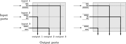
Figure 1: An input-queued switch, and two example matchings of inputs to outputs.

Figure 1 illustrates an input-queued switch with three input ports and three output ports. Packets arriving at input $k$ destined for output $\ell$ are stored at input port $k$, in queue $Q_{k,\ell}$, thus there are $N=9$ queues in total. (For this example, it is more natural to use double indexing, e.g., $Q_{3,2}$, whereas for general switched networks it is more natural to use single indexing, e.g., $Q_{i}$ for $1\leq i\leq N$.)

The switch operates in discrete time. At each time slot, the switch fabric can transmit a number of packets from input ports to output ports, subject to the two constraints that each input can transmit at most one packet, and that each output can receive at most one packet. In other words, at each time slot the switch can choose a matching from inputs to outputs. The schedule $\bolds{\sigma}\in\mathbb{R}_{+}^{3\times 3}$ is given by $\sigma_{k,\ell}=1$ if input port $k$ is matched to output port $\ell$ in a given time slot, and $\sigma_{k,\ell}=0$ otherwise. The matching constraints require that $\sum_{m=1}^{3}\sigma_{k,m}\leq 1$ for $k=1,2,3$, and $\sum_{m=1}^{3}\sigma_{m,\ell}\leq 1$ for $\ell=1,2,3$. Figure 1 shows two possible matchings. On the left-hand side, the matching allows a packet to be transmitted from input port 3 to output port 2, but since $Q_{3,2}$ is empty, no packet is actually transmitted.

In general, for an $n$-port switch, there are $N=n^{2}$ queues. The corresponding schedule set $\mathcal{S}$ is defined as

$$\mathcal{S}=\Biggl{\{}\bolds{\sigma}\in\{0,1\}^{n\times n}\dvtx\sum_{m=1}^{n}\sigma_{k,m}\leq 1,\sum_{m=1}^{n}\sigma_{m,\ell}\leq 1,1\leq k,\ell\leq n\Biggr{\}}.$$ (12)

It can be checked that $\mathcal{S}$ is monotone. Furthermore, due to Birkhoff–von Neumann theorem, BrK , VN , the convex hull of $\mathcal{S}$ is given by

$$\langle{\mathcal{S}}\rangle=\Biggl{\{}\mathbf{x}\in[0,1]^{n\times n}\dvtx\sum_{m=1}^{n}x_{k,m}\leq 1,\sum_{m=1}^{n}x_{m,\ell}\leq 1,1\leq k,\ell\leq n\Biggr{\}}.$$ (13)

Thus, the rank of $\langle{\mathcal{S}}\rangle$ is less than or equal to $2n=2\sqrt{N}$ for an $n$-port switch. Finally, given an arrival rate matrix $\bolds{\lambda}\in[0,1]^{n\times n}$, $\rho(\bolds{\lambda})$ is given by

$$\rho(\bolds{\lambda})=\max_{1\leq k,\ell\leq n}\Biggl{\{}\sum_{m=1}^{n}\lambda_{k,m},\sum_{m=1}^{n}\lambda_{m,\ell}\Biggr{\}}.$$

3 Related works

The question of determining the optimal scaling of queue sizes in switched networks, or more generally, stochastic processing networks, has been an important intellectual pursuit for more than a decade. The complexity of the generic stochastic processing network makes this task extremely challenging. Therefore, in search of tractable analysis, most of the prior work has been on trying to understand optimal scaling and scheduling policies for scaled systems: primarily, with respect to fluid and heavy-traffic scaling, that is, $\rho\to 1$.

In heavy-traffic analysis, one studies the queue-size behavior under a diffusion (or heavy-traffic) scaling. This regime was first considered by Kingman kingmanht ; since then, a substantial body of theory has developed, and modern treatments can be found in mike2 , bramson , williams , whittspl . Stolyar stolyar has studied a class of myopic scheduling policies, known as the maximum weight policy, introduced by Tassiulas and Ephremides tassiula1 , for a generalized switch model in the diffusion scaling. In a general version of the maximum weight policy, a schedule with maximum weight is chosen at each time step, with the weight of a schedule being equal to the sum of the weights of the queues chosen by that schedule. The weight of a queue is a function of its size. In particular, for the choice of one parameter class of functions parameterized by $\alpha>0$, $f(x)=x^{\alpha}$, the resulting class of policies are called the maximum weight policies with parameter $\alpha>0$, and denoted as MW-$\alpha$.

In stolyar , a complete characterization of the diffusion approximation for the queue-size process was obtained, under a condition known as “complete resource pooling,” when the network is operating under the MW-$\alpha$ policy, for any $\alpha>0$. Stolyar stolyar showed the remarkable result that the limiting queue-size vector lives in a one-dimensional state space. Operationally, this means that all one needs to keep track of is the one-dimensional total amount of work in the system (called the rescaled workload), and at any point in time one can assume that the individual queues have all been balanced. Furthermore, it was established that a max-weight policy minimizes the rescaled workload induced by any policy under the heavy-traffic scaling (with complete resource pooling). Dai and Lin LD05 , LD08 have established that a similar result holds (with complete resource pooling) in the more general setting of a stochastic processing network. In summary, under the complete resource pooling condition, the results in stolyar , LD05 , LD08 imply that the performance of the maximum weight policy in an input-queued switch, or more generally in a stochastic processing network, is always optimal (in the diffusion limit, and when each queue size is appropriately weighted). These results suggest that the average total queue-size scales as $1/(1-\rho)$ in the $\rho\to 1$ limit. However, such analyses do not capture the dependence on the network scheduling structure $\mathcal{S}$. Essentially, this is because the complete resource pooling condition reduces the system to a one-dimensional space (which may be highly dependent on a network’s structure), and optimality results are then initially expressed with respect to this one-dimensional space.

Motivated to capture the dependence of the queue sizes on the network scheduling structure $\mathcal{S}$, a heavy-traffic analysis of switched networks with multiple bottlenecks (without resource pooling) was pursued by Shah and Wischik SW . They established the so-called multiplicative state space collapse, and identified a member, denoted by MW-$0^{+}$ (obtained by taking $\alpha\to 0$), of the class of maximum-weight policies as optimal with respect to a critical fluid model. In a more recent work, Shah and Wischik SWo established the optimality of MW-$0^{+}$ with respect to overloaded fluid models as well. However, this collection of works stops short of establishing optimality for diffusion scaled queue-size processes.

Finally, we take note of the work by Meyn Meyn08 , which establishes that a class of generalized maximum weight policies achieve logarithmic [in $1/(1-\rho)$] regret with respect to an optimal policy under certain conditions.

In a related model—the bandwidth-sharing network model—Kang et al. kelly-williamsssc have established a diffusion approximation for the proportionally fair bandwidth allocation policy, assuming a technical “local traffic” condition, but without assuming complete resource pooling. They show that the resulting diffusion approximation has a product-form stationary distribution. Shah, Tsitsiklis and Zhong STZ have recently established that this product-form stationary distribution is indeed the limit of the stationary distributions of the original stochastic model (an interchange-of-limits result). As a consequence, if one could utilize a scheduling policy in a switched network that corresponds to the proportionally fair policy, then the resulting diffusion approximation will have a product-form stationary distribution, as long as the effective network scheduling structure $\mathcal{S}$ (precisely $\langle{\mathcal{S}}\rangle$) satisfies the “local traffic condition.” Now, proportional fairness is a continuous-time rate allocation policy that usually requires rate allocations that are a convex combination of multiple schedules. In a switched network, a policy must operate in discrete time and has to choose one schedule at any given time from a finite discrete set $\mathcal{S}$. For this reason, proportional fairness cannot be implemented directly. However, a natural randomized policy inspired by proportional fairness is likely to have the same diffusion approximation (since the fluid models would be identical, and the entire machinery of Kang et al. kelly-williamsssc , building upon the work of Bramson bramson and Williams williams , relies on a fluid model). As a consequence, if $\mathcal{S}$ (more accurately, $\langle{\mathcal{S}}\rangle$) satisfies the “local traffic condition,” then effectively the diffusion-scaled queue sizes would have a product-form stationary distribution, and would result in bounds similar to those implied by our results. In comparison, our results are nonasymptotic, in the sense that they hold for any admissible load, have a product-form structure, and do not require technical assumptions such as the “local traffic condition.” Furthermore, such generality is needed because there are popular examples, such as the input-queued switch, that do not satisfy the “local traffic condition.”

Another line of works—so-called large-deviations analysis—concerns exponentially decaying bounds on the tail probability of the steady-state distributions of queue sizes. Venkataramanan and Lin VL-LDP established that the maximum weight policy with weight parameter $\alpha>0$, MW-$\alpha$, optimizes the tail exponent of the $1+\alpha$ norm of the queue-size vector. Stolyar Stolyar-LDP showed that a so-called “exponential rule” optimizes the tail exponent of the max norm of the queue-size vector. However, these works do not characterize the tail exponent explicitly. See STZSIGM which has the best-known explicit bounds on the tail exponent.

In the context of input-queued switches, the example that has primarily motivated this work, the policy that we propose has the average total queue size bounded within factor $2$ of the same quantity induced by any policy, in the heavy-traffic limit. Furthermore, this result does not require conditions like complete resource pooling. More generally, our policy provides nonasymptotic bounds on queue sizes for every arrival rate and switch size. The policy even admits exponential tail bounds with respect to the stationary distribution, and the exponent of these tail bounds is optimal. These results are significant improvements to the state-of-the-art bounds for best performing policies for input-queued switches. As noted in the Introduction, our bound on the average total queue size is $\sqrt{N}$ times better than the existing bound for the maximum-weight policy, and $\log N/(1-\rho)$ times better than that for the batching policy in NeelyModiano . (Here $N$ is the number of queues, and $\rho$ the system load.) For further details of these results, see STZopen .

For a generic switched network, our policy induces average total queue size that scale linearly with the rank of $\langle{\mathcal{S}}\rangle$, under the diffusion scaling. This is in contrast to the best-known bounds, such as those for maximum weight policy, where the average queue-size scales as $N$, under the diffusion scaling. Therefore, whenever the rank of $\langle{\mathcal{S}}\rangle$ is smaller than $N$ (the number of queues), our policy provides tighter bounds. Under our policy, queue sizes admit exponential tail bounds. The bound on the distribution of queue sizes under our policy leads to an explicit characterization of the tail exponent, which is optimal for a wide range of single-hop switched networks, including input-queued switches and the independent-set model of wireless networks, when the underlying interference graph is perfect.

4 Insensitivity in stochastic networks

This section recalls the background on insensitive stochastic networks that underlies the main results of this work. We shall focus on descriptions of the insensitive bandwidth allocation in so-called bandwidth-sharing networks operating in continuous time. Properties of these insensitive networks are provided in the Appendix.

We consider a bandwidth-sharing network operating in continuous time with capacity constraints. The particular bandwidth-sharing policy of interest is the store-and-forward allocation (SFA) mentioned earlier. We shall use the SFA as an idealized policy to design online scheduling policies for switched networks. We now describe the precise model, the SFA policy, and its performance properties.

Model

Let time be continuous and indexed by $t\in\mathbb{R}_{+}$. Consider a network with $J\geq 1$ resources indexed from $1,\ldots,J$. Let there be $N$ routes, and suppose that each packet on route $i$ consumes an amount $R_{ji}\geq 0$ of resource $j$, for each $j\in\{1,2,\ldots,J\}$. Let $\mathcal{K}$ be the set of all resource–route pairs $(j,i)$ such that route $i$ uses resource $j$, that is, $\mathcal{K}=\{(j,i)\dvtx R_{ji}>0\}$. Without loss of generality, we assume that for each $i\in\{1,2,\ldots,N\}$, $\sum_{j=1}^{J}R_{ji}>0$. Let $\mathbf{R}$ be the $J\times N$ matrix with entries $R_{ji}$. Let $\mathbf{C}\in\mathbb{R}_{+}^{J}$ be a positive capacity vector with components $C_{j}$. For each route $i$, packets arrive as an independent Poisson process of rate $\lambda_{i}$. Packets arriving on route $i$ require a unit amount of service, deterministically.

We denote the number of packets on route $i$ at time $t$ by $M_{i}(t)$, and define the queue-size vector at time $t$ by $\mathbf{M}(t)=[M_{i}(t)]_{i=1}^{N}\in\mathbb{Z}_{+}^{N}$. Each packet gets service from the network at a rate determined according to a bandwidth-sharing policy. We also denote the total residual workload on route $i$ at time $t$ by $W_{i}(t)$, and let the vector of residual workload at time $t$ be $\mathbf{W}(t)=[W_{i}(t)]_{i=1}^{N}$. Once a packet receives its total (unit) amount of service, it departs the network.

We consider online, myopic bandwidth allocations. That is, the bandwidth allocation at time $t$ only depends on the queue-size vector $\mathbf{M}(t)$. When there are $m_{i}$ packets on route $i$, that is, if the vector of packets is $\mathbf{m}=[m_{i}]_{i=1}^{N}$, let the total bandwidth allocated to route $i$ be $\phi_{i}(\mathbf{m})\in\mathbb{R}_{+}$. We consider a processor-sharing policy, so that each packet on route $i$ is served at rate $\phi_{i}(\mathbf{m})/m_{i}$, if $m_{i}>0$. If $m_{i}=0$, let $\phi_{i}(\mathbf{m})=0$. If the bandwidth vector $\bolds{\phi}(\mathbf{m})=[\phi_{i}(\mathbf{m})]_{i=1}^{N}$ satisfies the capacity constraints

$$\mathbf{R}\bolds{\phi}(\mathbf{m})\leq\mathbf{C}\qquad\mbox{componentwise}$$ (14)

for all $\mathbf{m}\in\mathbb{Z}_{+}^{N}$, then, in light of Definition 2.2, we say that $\bolds{\phi}(\cdot)$ is an admissible bandwidth allocation. A Markovian description of the system is given by a process $\mathbf{Y}(t)$ which contains the queue-size vector $\mathbf{M}(t)$ along with the residual workloads of the set of packets on each route.

Now, on average, $\lambda_{i}$ units of work arrive to route $i$ per unit time. Therefore, in order for the Markov process $\mathbf{Y}(\cdot)$ to be positive (Harris) recurrent, it is necessary that

$$\mathbf{R}\bolds{\lambda} < \mathbf{C}\qquad\mbox{componentwise}.$$ (15)

All such $\bolds{\lambda}=[\lambda_{i}]_{i=1}^{N}\in\mathbb{R}_{+}^{N}$ will be called strictly admissible, in the same spirit as strictly admissible vectors for a switched network. Similarly to the corresponding switched network, given $\bolds{\lambda}\in\mathbb{R}_{+}^{N}$, we can define $\rho(\bolds{\lambda})$, the load induced by $\bolds{\lambda}$, using (10), as well as $\tilde{\rho}_{j}=(\sum_{i}R_{ji}\lambda_{i})/C_{j}$. Then by Lemma 2.4, $\rho(\bolds{\lambda})=\max_{j}\tilde{\rho}_{j}$, where $\tilde{\rho}_{j}$ can be interpreted as the load induced by $\bolds{\lambda}$ on resource $j$.

Store-and-forward allocation (SFA) policy

We describe the store-and-forward allocation policy that was first considered by Massoulié and later analyzed in the thesis of Proutière PTh . Bonald and Proutière bonaldproutiere2 established that this policy induces product-form stationary distributions and is insensitive with respect to phase-type distributions. This policy is shown to be insensitive for general service time distributions, including the deterministic service considered here, by Zachary zachary . The relation between this policy, the proportionally fair allocation, and multi-class queuing networks is discussed in depth by Walton walton and Kelly, Massoulié and Walton KMW . The insensitivity property implies that the invariant measure of the process $\mathbf{M}(t)$ only depends on the parameters $\bolds{\lambda}=[\lambda_{i}]_{i=1}^{N}\in\mathbb{R}_{+}^{N}$, and no other aspects of the stochastic description of the system.

We first give an informal motivation for SFA. SFA is closely related to quasi-reversible queuing networks. Consider a continuous-time multi-class queuing network (without scheduling constraints) consisting of processor sharing queues indexed by $j\in\{1,\ldots,J\}$ and job types indexed by the routes $i\in\{1,\ldots,N\}$. Each route $i$ job has a service requirement $R_{ji}$ at each queue $j$, and a fixed service capacity $C_{j}$ is shared between jobs at the queue. Here each job will sequentially visit all the queues (so-called store-and-forward) and will visit each queue a fixed number of times. If we assume that jobs on each route arrive as a Poisson process, then the resulting queuing network will be stable for all strictly admissible arrival rates. Moreover, each stationary queue will be independent with a queue size that scales, with its load $\rho$, as $\rho/(1-\rho)$. For further details, see Kelly Ke79 . So, assuming each queue has equal load, the total number of jobs within the network is of the order $J\rho/(1-\rho)$. In other words, these networks have the stability and queue-size scaling that we require, but do not obey the necessary scheduling constraints (14). However, these networks do produce an admissible schedule on average. For this reason, we consider an SFA policy which, given the number of jobs on each route, allocates the average rate with which jobs are transferred through this multi-class network. Next, we describe this policy (using notation similar to those used in KMW , walton ).

Given $\mathbf{m}\in\mathbb{Z}_{+}^{N}$, define

$$U(\mathbf{m})=\biggl{\{}\tilde{\mathbf{m}}=\bigl{(}\tilde{m}_{ji}\dvtx(j,i)\in\mathcal{K}\bigr{)}\in\mathbb{Z}_{+}^{|\mathcal{K}|}\dvtx\sum_{j\dvtx j\in i}\tilde{m}_{ji}=m_{i},\mbox{ for all }1\leq i\leq N\biggr{\}}.$$

For $\mathbf{L}\in\mathbb{Z}_{+}^{J}$, we also define

$$V(\mathbf{L})=\biggl{\{}\tilde{\mathbf{m}}=\bigl{(}\tilde{m}_{ji}\dvtx(j,i)\in\mathcal{K}\bigr{)}\in\mathbb{Z}_{+}^{|\mathcal{K}|}\dvtx\sum_{i\dvtx i\ni j}\tilde{m}_{ji}=L_{j},\mbox{ for all }1\leq j\leq J\biggr{\}}.$$

Here, by notation $j\in i$ (and $i\ni j$) we mean $R_{ji}>0$. For each $\tilde{\mathbf{m}}\in U(\mathbf{m})$, we exploit notation somewhat and define $\tilde{m}_{j}=\sum_{i\dvtx j\in i}\tilde{m}_{ji}$, for all $j\leq J$. Also define

$$\pmatrix{\tilde{m}_{j}\vspace*{2pt}\cr\tilde{m}_{ji}\dvtx i\ni j}=\frac{\tilde{m}_{j}!}{\prod_{i\dvtx j\in i}(\tilde{m}_{ji}!)}.$$

For $\mathbf{m}\in\mathbb{Z}_{+}^{N}$, we define $\Phi(\mathbf{m})$ as

$$\Phi(\mathbf{m})=\sum_{\tilde{\mathbf{m}}\in U(\mathbf{m})}\prod_{j\in J}\biggl{(}\pmatrix{\tilde{m}_{j}\vspace*{2pt}\cr\tilde{m}_{ji}\dvtx i\ni j}\prod_{i\dvtx j\in i}\biggl{(}\frac{R_{ji}}{C_{j}}\biggr{)}^{\tilde{m}_{ji}}\biggr{)}.$$ (16)

We shall define $\Phi(\mathbf{m})=0$ if any of the components of $\mathbf{m}$ is negative. The store-and-forward allocation (SFA) assigns rates according to the function $\bolds{\phi}\dvtx\mathbb{Z}_{+}^{N}\to\mathbb{R}_{+}^{N}$, so that for any $\mathbf{m}\in\mathbb{Z}_{+}^{N}$, $\bolds{\phi}(\mathbf{m})=(\phi_{i}(\mathbf{m}))_{i=1}^{N}$, with

$$\phi_{i}(\mathbf{m})=\frac{\Phi(\mathbf{m}-\mathbf{e}_{i})}{\Phi(\mathbf{m})},$$ (17)

where, recalling that $\mathbf{m}-\mathbf{e}_{i}$ is the same as $\mathbf{m}$ at all but the $i$th component, its $i$th component equals $m_{i}-1$. The bandwidth allocation $\bolds{\phi}(\mathbf{m})$ is the stationary throughput of jobs on the routes of a multi-class queuing network (described above), conditional on there being $\mathbf{m}$ jobs on each route.

A priori it is not clear if the above described bandwidth allocation is even admissible, that is, satisfies (14). This can be argued as follows. The $\bolds{\phi}(\mathbf{m})$ can be related to the stationary throughput of a multi-class network with a finite number of jobs, $\mathbf{m}$, on each route. Under this scenario (due to finite number of jobs), each queue must be stable. Therefore, the load on each queue, $\mathbf{R}\bolds{\phi}(\mathbf{m})$, must be less than the overall system capacity $\mathbf{C}$. That is, the allocation is admissible. The precise argument along these lines is provided in, for example, KMW , Corollary 2 and walton , Lemma 4.1.

The SFA induces a product-form invariant distribution for the number of packets waiting in the bandwidth-sharing network and is insensitive. We summarize this in the following result.

Theorem 4.1

Consider a bandwidth-sharing network with $\mathbf{R}\bolds{\lambda}<\mathbf{C}$. Under the SFA policy described above, the Markov process $\mathbf{Y}(t)$ is positive (Harris) recurrent, and $\mathbf{M}(t)$ has a unique stationary probability distribution ${\bolds{\pi}}$ given by

$${\bolds{\pi}}(\mathbf{m})=\frac{\Phi(\mathbf{m})}{\Phi}\prod_{i=1}^{N}\lambda_{i}^{m_{i}}\qquad\mbox{for all }\mathbf{m}\in\mathbb{Z}_{+}^{N},$$ (18)

where

$$\Phi=\prod_{j=1}^{J}\biggl{(}\frac{C_{j}}{C_{j}-\sum_{i\dvtx i\ni j}R_{ji}\lambda_{i}}\biggr{)}$$ (19)

is a normalizing factor. Furthermore, the steady-state residual workload of packets waiting in the network can be characterized as follows. First, the steady-state distribution of the residual workload of a packet is independent from ${\bolds{\pi}}$. Second, in steady state, conditioned on the number of packets on each route of the network, the residual workload of each packet is uniformly distributed on $[0,1]$, and is independent from the residual workloads of other packets.

Note that statements similar to Theorem 4.1 have appeared in other works, for example, bonaldproutiere1 , walton , Proposition 4.2, and KMW . Theorem 4.1 is a summary of these statements, and for completeness, it is proved in Appendix A.

The following property of the stationary distribution ${\bolds{\pi}}$ described in Theorem 4.1 will be useful.

Proposition 4.2

Consider the setup of Theorem 4.1, and let ${\bolds{\pi}}$ be described by (18). Define a measure $\tilde{{\bolds{\pi}}}$ on $\mathbb{Z}_{+}^{|\mathcal{K}|}$ as follows: for $\tilde{\mathbf{m}}\in\mathbb{Z}_{+}^{|\mathcal{K}|}$,

$$\tilde{{\bolds{\pi}}}(\tilde{\mathbf{m}}) = \frac{1}{\Phi}\prod_{j=1}^{J}\biggl{(}\pmatrix{\tilde{m}_{j}\vspace*{2pt}\cr\tilde{m}_{ji}\dvtx i\ni j}\prod_{i\dvtx j\in i}\biggl{(}\frac{R_{ji}\lambda_{i}}{C_{j}}\biggr{)}^{\tilde{m}_{ji}}\biggr{)}.$$ (20)

Then, for any $L\in\mathbb{Z}_{+}$,

$${\bolds{\pi}}\Biggl{(}\Biggl{\{}\mathbf{m}\dvtx\sum_{i=1}^{N}m_{i}=L\Biggr{\}}\Biggr{)} = \tilde{{\bolds{\pi}}}\Biggl{(}\Biggl{\{}\tilde{\mathbf{m}}\dvtx\sum_{j=1}^{J}\tilde{m}_{j}=L\Biggr{\}}\Biggr{)}.$$ (21)

We relate the distribution $\tilde{{\bolds{\pi}}}$ to the stationary distribution of an insensitive multi-class queuing network with a product-form stationary distribution and geometrically distributed queue sizes.

Proposition 4.3

Consider the distribution $\tilde{{\bolds{\pi}}}$ defined in (20). Then, for any $\mathbf{L}=(L_{1},\ldots,L_{J})\in\mathbb{Z}_{+}^{J}$,

$$\qquad\tilde{{\bolds{\pi}}}(\tilde{m}_{1}=L_{1},\ldots,\tilde{m}_{J}=L_{J}) = \sum_{(\tilde{m}_{ji})\in V(\mathbf{L})}\tilde{{\bolds{\pi}}}\bigl{(}(\tilde{m}_{ji})\bigr{)}=\prod_{j=1}^{J}\tilde{\rho}_{j}^{L_{j}}(1-\tilde{\rho}_{j}),$$ (22)

where $\tilde{\rho}_{j}=(\sum_{i\dvtx i\ni j}R_{ji}\lambda_{j})/C_{j}$.

Using Theorem 4.1 and Propositions 4.2 and 4.3, we can compute the expected value and the probability tail exponent of the steady-state total residual workload in the system. Recall that the total residual workload in the system at time $t$ is given by $\sum_{i=1}^{N}W_{i}(t)$.

Proposition 4.4

Consider a bandwidth-sharing network with $\mathbf{R}\bolds{\lambda}<\mathbf{C}$, operating under the SFA policy. Denote the load induced by $\bolds{\lambda}$ to be $\rho=\rho(\bolds{\lambda})(<1)$, and for each $j$, let $\tilde{\rho}_{j}=(\sum_{i}R_{ji}\lambda_{i})/C_{j}$. Then $\mathbf{W}(\cdot)$ has a unique stationary probability distribution. With respect to this stationary distribution, the following properties hold: [(ii)]

The expected total residual workload is given by

$$\mathbb{E}\Biggl{[}\sum_{i=1}^{N}W_{i}\Biggr{]}=\frac{1}{2}\sum_{j=1}^{J}\frac{\tilde{\rho}_{j}}{1-\tilde{\rho}_{j}}.$$ (23)

The distribution of the total residual workload has an exponential tail with exponent given by

$$\lim_{L\to\infty}\frac{1}{L}\log\mathbb{P}\Biggl{(}\sum_{i=1}^{N}W_{i}\geq L\Biggr{)}=-\theta^{*},$$ (24)

where $\theta^{*}$ is the unique positive solution of the equation $\rho(e^{\theta}-1)=\theta$.

5 Main result: A policy and its performance

In this section, we describe an online scheduling policy and quantify its performance in terms of explicit, closed-form bounds on the stationary distribution of the induced queue sizes. Section 5.1 describes the policy for a generic switched network and provides the statement of the main result. Section 5.2 discusses its implications. Specifically, it discusses (a) the optimality of the policy for a large class of switched networks with respect to exponential tail bounds, and (b) the optimality of the policy for a class of switched networks, including input-queued switches, with respect to the average total queue size. Section 5.3 proves the main result stated in Section 5.1.

5.1 A policy for switched networks

The basic idea behind the policy, to be described in detail shortly, is as follows. Given a switched network, denoted by SN, with constraint set $\mathcal{S}$ and $N$ queues, let $\langle{\mathcal{S}}\rangle$ have rank $J$ and representation [cf. (6)]

$$\langle{\mathcal{S}}\rangle=\bigl{\{}\mathbf{x}\in[0,1]^{N}\dvtx\mathbf{R}\mathbf{x}\leq\mathbf{C}\bigr{\}},\qquad\mathbf{R}\in\mathbb{R}_{+}^{N\times J},\mathbf{C}\in\mathbb{R}_{+}^{J}.$$

Now consider a virtual bandwidth-sharing network, denoted by BN, with $N$ routes corresponding to each of these $N$ queues. The resource–route relation is determined precisely by the matrix $\mathbf{R}$, and the $J$ resources have capacities given by $\mathbf{C}$. Both networks, SN and BN, are fed identical arrivals. That is, whenever a packet arrives to queue $i$ in SN, a packet is added to route $i$ in BN at the same time. The main question is that of determining a scheduling policy for SN; this will be derived from BN. Specifically, BN will operate under the insensitive SFA policy described in Section 4. By Theorem 4.1 and Propositions 4.2 and 4.3, this will induce a desirable stationary distribution of queue sizes in BN. Therefore, if we could use the rate allocation of BN, that is, the SFA policy, directly in SN, it would give us a desired performance in terms of the stationary distribution of the induced queue sizes. Now the rate allocation in BN is such that the instantaneous rate is always inside $\langle{\mathcal{S}}\rangle$. However, it could change all the time and need not utilize points of $\mathcal{S}$ as rates. In contrast, in SN we require that the rate allocation can change only once per discrete time slot and it must always employ one of the generators of $\langle{\mathcal{S}}\rangle$, that is, a schedule from $\mathcal{S}$. The key to our policy is an effective way to emulate the rate allocation of BN under SFA (or for that matter, any admissible bandwidth allocation) by utilizing schedules from $\mathcal{S}$ in an online manner and with the discrete-time constraint. We will see shortly that this emulation policy relies on $\mathcal{S}$ being monotone; cf. Assumption 2.1.

To that end, we describe this emulation policy. Let us start by introducing some useful notation. Let $\mathbf{A}(\cdot)=(A_{i}(\cdot))$ be the vector of exogenous, independent Poisson processes according to which unit-sized packets arrive to both BN and SN, simultaneously. Recall that $A_{i}(\cdot)$ is a Poisson process with rate $\lambda_{i}$. Let $\mathbf{M}(t)=(M_{i}(t))$ denote the vector of numbers of packets waiting on the $N$ routes in BN at time $t\geq 0$. In BN, the services are allocated according to the SFA policy described in Section 4. Let $\Lambda^{\mathrm{SFA}}(\cdot)=(\Lambda^{\mathrm{SFA}}_{i}(\cdot))\in\mathbb{R}_{+}^{N}$ denote the cumulative amount of service allocated to the $N$ routes in BN under the SFA policy: $\Lambda^{\mathrm{SFA}}_{i}(t)$ denotes the total amount of service allocated to all packets on route $i$ during the interval $[0,t]$, for $t\geq 0$, with $\Lambda^{\mathrm{SFA}}_{i}(0)=0$ for $1\leq i\leq N$. By definition, all components of $\Lambda^{\mathrm{SFA}}(\cdot)$ are nondecreasing and Lipschitz continuous. Furthermore, $(\Lambda^{\mathrm{SFA}}(t+s)-\Lambda^{\mathrm{SFA}}(t))/s\in\langle{\mathcal{S}}\rangle$ for any $t\geq 0$ and $s>0$. Recall that the (right-)derivative of $\Lambda^{\mathrm{SFA}}(\cdot)$ is determined by $\mathbf{M}(\cdot)$ through the function $\bolds{\phi}(\cdot)$ as defined in (17).

Now we describe the scheduling policy for SN that will rely on $\Lambda^{\mathrm{SFA}}(\cdot)$. Let $\mathbf{B}(\tau)=(B_{i}(\tau))$ denote the cumulative amount of service allocated in SN by the scheduling policy up to time slot $\tau\geq 0$, with $\mathbf{B}(0)=\mathbf{0}$. The scheduling policy determines how $\mathbf{B}(\cdot)$ is updated. Let $\mathbf{Q}(\tau)=(Q_{i}(\tau))$ be the queue sizes measured at the end of time slot $\tau$. Let service be provided according to the scheduling policy instantly at the beginning of a time slot. Thus, the scheduling policy decides the schedule $d\mathbf{B}(\tau)=\mathbf{B}(\tau+1)-\mathbf{B}(\tau)\in\mathcal{S}$ at the very beginning of time slot $\tau+1$. This decision is made as follows. Let $\mathbf{D}(\tau)=\Lambda^{\mathrm{SFA}}(\tau)-\mathbf{B}(\tau)$. We will see shortly that under our policy, $\mathbf{D}(\tau)$ is always nonnegative. This fact will be useful at various places, and in particular, for bounding the discrepancy between the continuous-time policy SFA and its discrete-time emulation. Let $\rho(\mathbf{D}(\tau))$ be the optimal objective value in the optimization problem $\mathrm{PRIMAL}(\mathbf{D}(\tau))$ defined in (7). In particular, there exists a nonnegative combination of schedules in $\mathcal{S}$ such that

$$\sum_{\bolds{\sigma}\in\mathcal{S}}\tilde{\alpha}_{\bolds{\sigma}}\bolds{\sigma}\geq\mathbf{D}(\tau)\quad\mbox{and}\quad\sum_{\bolds{\sigma}\in\mathcal{S}}\tilde{\alpha}_{\bolds{\sigma}}=\rho\bigl{(}\mathbf{D}(\tau)\bigr{)}.$$ (25)

We claim that in fact, we can find nonnegative numbers $\alpha_{\bolds{\sigma}}$, $\bolds{\sigma}\in\mathcal{S}$, such that

$$\sum_{\bolds{\sigma}\in\mathcal{S}}\alpha_{\bolds{\sigma}}\bolds{\sigma}=\mathbf{D}(\tau)\quad\mbox{and}\quad\sum_{\bolds{\sigma}\in\mathcal{S}}\alpha_{\bolds{\sigma}}=\rho\bigl{(}\mathbf{D}(\tau)\bigr{)}.$$ (26)

This is formalized in the following lemma.

Lemma 5.1

Let $\mathbf{D}\in\mathbb{R}_{+}^{N}$ be a nonnegative vector. Consider the static planning problem $\mathrm{PRIMAL}(\mathbf{D})$ defined in (7). Let the optimal objective value to $\mathrm{PRIMAL}(\mathbf{D})$ be $\rho(\mathbf{D})$. Then there exists $\alpha_{\bolds{\sigma}}\geq 0$, $\bolds{\sigma}\in\mathcal{S}$, such that (26) holds.

The proof of the lemma relies on Assumption 2.1, and is provided in the Appendix.

There could be many possible nonnegative combinations of $\mathbf{D}(\tau)$ satisfying (26). If there exist nonnegative numbers $\alpha_{\bolds{\sigma}}$, $\bolds{\sigma}\in\mathcal{S}$, satisfying (26) with $\alpha_{\bolds{\sigma}^{\prime}}\geq 1$ for some $\bolds{\sigma}^{\prime}\in\mathcal{S}$, then choose $\bolds{\sigma}^{\prime}$ as the schedule: set $d\mathbf{B}(\tau)=\bolds{\sigma}^{\prime}$. If no such decomposition exists for $\mathbf{D}(\tau)$, then set $d\mathbf{B}(\tau)=\tilde{\bolds{\sigma}}$, where $\tilde{\bolds{\sigma}}$ is a solution (ties broken arbitrarily) of

$$\mbox{maximize}\qquad\sum_{i}\sigma_{i}\quad\mbox{over}\quad\bolds{\sigma}\in\mathcal{S},\bolds{\sigma}\leq\mathbf{D}(\tau).$$ (27)

Here first observe that for all time $\tau$, $d\mathbf{B}(\tau)\leq\mathbf{D}(\tau)$, so $\mathbf{D}(\tau)\geq\mathbf{0}$. Hence, $\mathbf{0}$ is a feasible solution for the above problem, as $\mathbf{0}\in\mathcal{S}$.

The above is a complete description of the scheduling policy. Observe that it is an online policy, as the virtual network BN can be simulated in an online manner, and, given this, the scheduling decision in SN relies only on the history of BN and SN. The following result quantifies the performance of the policy.

Theorem 5.2

Given a strictly admissible arrival rate vector $\bolds{\lambda}$, with $\rho=\rho(\bolds{\lambda})<1$, under the policy described above, the switched network SN is positive recurrent and has a unique stationary distribution. Let $\tilde{\rho}_{j}=\break(\sum_{i}R_{ji}\lambda_{i})/C_{j}$, $j=1,2,\ldots,J$ be the same as in Proposition 4.4. With respect to this stationary distribution, the following properties hold: [(2)]

The expected total queue size is bounded as

$$\mathbb{E}\Biggl{[}\sum_{i=1}^{N}Q_{i}\Biggr{]} \leq \frac{1}{2}\Biggl{(}\sum_{j=1}^{J}\frac{\tilde{\rho}_{j}}{1-\tilde{\rho}_{j}}\Biggr{)}+K(N+2),$$ (28)

where $K=\max_{\bolds{\sigma}\in\mathcal{S}}(\sum_{i}\sigma_{i})$.

The distribution of the total queue size has an exponential tail with exponent given by

$$\lim_{L\to\infty}\frac{1}{L}\log\mathbb{P}\Biggl{(}\sum_{i=1}^{N}Q_{i}\geq L\Biggr{)} = -\theta^{*},$$ (29)

where $\theta^{*}$ is the unique positive solution of the equation $\rho(e^{\theta}-1)=\theta$.

5.2 Optimality of the policy

This section establishes the optimality of our policy for input-queued switches, both with respect to expected total queue-size scaling and tail exponent. General conditions under which our policy is optimal with respect to tail exponent are also provided.

Scaling of queue sizes

We start by formalizing what we mean by the optimality of expected queue sizes and of their tail exponents. We consider policies under which there is a well-defined limiting stationary distribution of the queue sizes for all $\bolds{\lambda}$ such that $\rho(\bolds{\lambda})<1$. Note that the class of policies is not empty; indeed, the maximum weight policy and our policy are members of this class. With some abuse of notation, let ${\bolds{\pi}}$ denote the stationary distribution of the queue-size vector under the policy of interest. We are interested in two quantities: [(2)]

Expected total queue size. Let $\overline{Q}$ be the expected total queue size under the stationary distribution ${\bolds{\pi}}$, defined by

$$\overline{Q}=\mathbb{E}_{{\bolds{\pi}}}\biggl{[}\sum_{i}Q_{i}\biggr{]}.$$

Note that by ergodicity, the time average of the total queue size and the expected total queue size under ${\bolds{\pi}}$ are the same quantity.

Tail exponent. Let $\beta_{L}(Q),\beta_{U}(Q)\in[-\infty,0]$ be the lower and upper limits of the tail exponent of the total queue size under ${\bolds{\pi}}$ (possibly $-\infty$ or $0$), respectively, defined by

$$\beta_{L}(Q) = \lim\inf_{\ell\to\infty}\frac{1}{\ell}\log\mathbb{P}_{{\bolds{\pi}}}\biggl{(}\sum_{i}Q_{i}\geq\ell\biggr{)}\quad\mbox{and}$$ (30)

$$\beta_{U}(Q) = \lim\sup_{\ell\to\infty}\frac{1}{\ell}\log\mathbb{P}_{{\bolds{\pi}}}\biggl{(}\sum_{i}Q_{i}\geq\ell\biggr{)}.$$ (31)

If $\beta_{L}(Q)=\beta_{U}(Q)$, then we denote this common value by $\beta(Q)$. We are interested in policies that can achieve minimal $\overline{Q}$ and $\beta(Q)$. For tractability, we focus on scalings of these quantities with respect to $\mathcal{S}$ (equivalently, $N$) and $\rho(\bolds{\lambda})$, as $1/(1-\rho(\bolds{\lambda}))$ and $N$ increase. For different $\bolds{\lambda}^{\prime}$ and $\bolds{\lambda}$, it is possible that $\rho(\bolds{\lambda})=\rho(\bolds{\lambda}^{\prime})$, but the scaling of $\overline{Q}$, for example, could be wildly different. For this reason, we consider the worst possible dependence on $1/(1-\rho)$ and $N$ among all $\bolds{\lambda}$ with $\rho(\bolds{\lambda})=\rho$.

Note that we are considering scalings with respect to two quantities, $\rho$ and $N$, and we are interested in two limiting regimes, $\rho\to 1$ and $N\to\infty$. The optimality of queue-size scaling stated here is with respect to the order of limits $\rho\to 1$ and then $N\to\infty$. As noted in STZopen , taking the limits in different orders could potentially result in different limiting behaviors of the object of interest, for example, $\overline{Q}$. For further discussion, see Section 6. It should be noted, however, that whenever the tail exponent is optimal, this optimality holds for any $\rho$ and $N$.

Optimality of the tail exponent

Here we establish sufficient conditions under which our policy is optimal with respect to tail exponent. First, we present a universal lower bound on the tail exponent, for a general single-hop switched network under any policy. We then provide a condition under which this lower bound matches the tail exponent under our policy. This condition is satisfied by both input-queued switches and the independent-set model of wireless networks.

Consider any policy under which there exists a well-defined limiting stationary distribution of the queue sizes for all $\bolds{\lambda}$ such that $\rho(\bolds{\lambda})<1$. Let ${\bolds{\pi}}_{0}$ denote the stationary distribution of queue sizes under this policy. The following lemma establishes a universal lower bound on the tail exponent.

Lemma 5.3

Consider a switched network as described in Theorem 5.2, with scheduling set $\mathcal{S}$ and admissible region $\{\mathbf{x}\in[0,1]^{N}\dvtx\mathbf{R}\mathbf{x}\leq\mathbf{C}\}$. Let ${\bolds{\pi}}_{0}$ and $\bolds{\lambda}$ be as described. For each $j$, let $\tilde{\rho}_{j}=\sum_{i=1}^{N}R_{ji}\lambda_{i}/C_{j}$ be defined as in Theorem 5.2. Then under ${\bolds{\pi}}_{0}$,

$$\liminf_{L\to\infty}\frac{1}{L}\log\mathbb{P}_{{\bolds{\pi}}_{0}}\biggl{(}\sum_{i}Q_{i}\geq L\biggr{)}\geq-\min_{j=1,2,\ldots,J}\theta^{*}_{j},$$ (32)

where, for each $j\in\{1,2,\ldots,J\}$, $\theta^{*}_{j}$ is the unique positive solution of the equation

$$\sum_{i=1}^{N}\lambda_{i}\bigl{(}e^{R_{ji}\theta}-1\bigr{)}=\theta.$$

Consider a fixed $j\in\{1,2,\ldots,J\}$. Without loss of generality, we assume that $C_{j}=1$, by properly normalizing the inequality $(\mathbf{R}\mathbf{x})_{j}\leq C_{j}$. In this case, $R_{ji}\leq 1$ for all $i$, since for each $i\in\{1,2,\ldots,N\}$, $\mathbf{e}_{i}\in\mathcal{S}\subset\langle{\mathcal{S}}\rangle$, and satisfies the constraint $(\mathbf{R}\mathbf{e}_{i})_{j}=R_{ji}\leq C_{j}=1$.

Now consider the following single-server queuing system. The arrival process is given by the sum $\sum_{i=1}^{N}R_{ji}A_{i}(\cdot)$, so that arrivals across time slots are independent, and that in each time slot, the amount of work that arrives is $\sum_{i=1}^{N}R_{ji}a_{i}$, where $a_{i}$ is an independent Poisson random variable with mean $\lambda_{i}$, for each $i$. Note that the arriving amount in a single time slot does not have to be integral. Note also that $\sum_{i=1}^{N}R_{ji}\lambda_{i}=\tilde{\rho}_{j}<1$, since $\rho(\bolds{\lambda})=\max_{j}\tilde{\rho}_{j}<1$. In each time slot, a unit amount of service is allocated to the total workload in the system. Then, for this system, the workload process $W(\cdot)$ satisfies

$$W(\tau+1)=\bigl{[}W(\tau)-1\bigr{]}^{+}+\sum_{i=1}^{N}R_{ji}a_{i}(\tau),$$

where $a_{i}(\tau)$ is the number of arrivals to queue $i$ in the original system in time slot $\tau$. We make two observations for this system. First, $W(\cdot)$ is stochastically dominated by $\sum_{i=1}^{N}R_{ji}Q_{i}(\cdot)$, where $Q_{i}(\cdot)$ is the size of queue $i$ in the original system, under any online scheduling policy. This is because for all schedules $\bolds{\sigma}\in\mathcal{S}$, $\bolds{\sigma}$ satisfies $\mathbf{R}\bolds{\sigma}\leq\mathbf{C}$, and hence $\sum_{i=1}^{N}R_{ji}\sigma_{i}\leq C_{j}=1$ for every $\bolds{\sigma}\in\mathcal{S}$. Second, since $R_{ji}\leq 1$ for all $i$, $\sum_{i=1}^{N}R_{ji}Q_{i}(\cdot)$ is stochastically dominated by $\sum_{i=1}^{N}Q_{i}(\cdot)$. Thus we have

$$\liminf_{L\to\infty}\frac{1}{L}\log\mathbb{P}_{{\bolds{\pi}}_{0}}\biggl{(}\sum_{i}Q_{i}\geq L\biggr{)}\geq\liminf_{L\to\infty}\frac{1}{L}\log\mathbb{P}\bigl{(}W(\infty)\geq L\bigr{)}.$$

We now show that

$$\liminf_{L\to\infty}\frac{1}{L}\log\mathbb{P}\bigl{(}W(\infty)\geq L\bigr{)}\geq-\theta^{*}_{j},$$

where $\theta^{*}_{j}$ is the unique positive solution of the equation

$$\sum_{i=1}^{N}\lambda_{i}\bigl{(}e^{R_{ji}\theta}-1\bigr{)}=\theta.$$

Consider the log-moment generating function (log-MGF) of $\sum_{i=1}^{N}R_{ji}a_{i}$, the arriving amount in one time slot. Since $a_{i}$ is a Poisson random variable with mean $\lambda_{i}$ for each $i$, its moment generating function is given by

$$f(\theta)=\exp\Biggl{(}\sum_{i=1}^{N}\lambda_{i}\bigl{(}e^{R_{ji}\theta}-1\bigr{)}\Biggr{)}.$$

Hence the log-MGF is

$$\log f(\theta)=\sum_{i=1}^{N}\lambda_{i}\bigl{(}e^{R_{ji}\theta}-1\bigr{)}.$$

By Theorem 1.4 of bigQ ,

$$\lim_{L\to\infty}\frac{1}{L}\log\mathbb{P}\bigl{(}W(\infty)\geq L\bigr{)}=-\theta^{*}_{j},$$

where $\theta^{*}_{j}=\sup\{\theta>0\dvtx\log f(\theta)<\theta\}$. Since $\log f(\theta)-\theta$ is strictly convex, $\theta^{*}_{j}$ satisfies

$$\sum_{i=1}^{N}\lambda_{i}\bigl{(}e^{R_{ji}\theta^{*}_{j}}-1\bigr{)}=\theta^{*}_{j}.$$

$j\in\{1,2,\ldots,J\}$ is arbitrary, so

$$\liminf_{L\to\infty}\frac{1}{L}\log\mathbb{P}_{{\bolds{\pi}}_{0}}\biggl{(}\sum_{i}Q_{i}\geq L\biggr{)}\geq-\min_{j=1,2,\ldots,J}\theta^{*}_{j}.$$

For general switched networks, the lower bound above need not match the tail exponent achieved under our policy [cf. (29)]. However, for a wide class of switched networks, these two quantities are equal. The following corollary of Lemma 5.3 is immediate.

Corollary 5.4

Consider a switched network as described in Lemma 5.3, with scheduling set $\mathcal{S}$ and admissible region $\{\mathbf{x}\in[0,1]^{N}\dvtx\mathbf{R}\mathbf{x}\leq\mathbf{1}\}$. If for all $j$ and $i$, $R_{ji}\in\{0,1\}$, then our policy achieves optimal tail exponent, for any strictly admissible arrival-rate vector $\bolds{\lambda}$.

Let $\bolds{\lambda}\in\mathbb{R}_{+}^{N}$ be strictly admissible, that is, $\mathbf{R}\bolds{\lambda}<\mathbf{1}$. Let $\tilde{\rho}_{j}=\sum_{i}R_{ji}\lambda_{i}$ for each $j$, and let $\rho=\rho(\bolds{\lambda})$ be the system load induced by $\bolds{\lambda}$. Consider the $\theta^{*}_{j}$ in Lemma 5.3. When $R_{ji}\in\{0,1\}$ for all $j$, and $i$, $\theta^{*}_{j}$ is the unique positive solution of the equation

$$\tilde{\rho}_{j}\bigl{(}e^{\theta}-1\bigr{)}=\theta$$

for each $j$. Using the relation $\rho=\max_{j}\tilde{\rho}_{j}$, we see that $\min_{j}\theta^{*}_{j}$ is the unique positive solution of the equation

$$\rho\bigl{(}e^{\theta}-1\bigr{)}=\theta.$$

Comparing this with equation (29) of Theorem 5.2, we see that our policy achieves the optimal tail exponent. Consider an $n\times n$ input-queued switch, defined in Section 2.4, and with the admissible region described by (13). By Corollary 5.4, it is clear that the tail exponent in input-queued switches is optimal under our policy. Moreover, input-queued switches are not the only network model that satisfies the condition stated in Corollary 5.4. For example, consider the independent-set model of a wireless network. When the underlying interference graph is bipartite, it is easy to see that the admissible region is characterized by inequalities of the form $x_{i}+x_{j}\leq 1$ over all edges $(i,j)$ of the graph, and $x_{i}\leq 1$ for isolated nodes $i$. More generally, when the underlying graph is perfect, inequality constraints characterizing the admissible region take the form $\sum_{i}x_{i}\leq 1$, where the summation is over all vertices of a clique. This latter fact follows from a proof of the weak perfect graph theorem, see, for example, Theorem 12.1.2 in Matousek2002 . Thus the incidence matrix $\mathbf{R}$ has all entries in $\{0,1\}$, and the tail exponent under our policy is optimal for this model.

Optimality in input-queued switches

Here we argue the optimality of our policy for input-queued switches. As discussed above, the scaling of tail exponent is optimal under our policy for input-queued switches. We would argue the optimal scaling of the average total queue size under our policy for input-queued switches. To that end, as argued in Shah, Tsitsiklis and Zhong STZopen , when all input and output ports approach critical load, the average total queue size under any policy for input-queued switch must scale at least as fast as $\sqrt{N}/(1-\rho)$, for any $n$-port switch with $N=n^{2}$ queues. For completeness, we include the proof for this lower bound here. As in Section 2.4, we use double indexing.

Lemma 5.5

Consider an $n$-port input-queued switch, with an arrival rate vector $\bolds{\lambda}$. Suppose that the loads on all input and output ports are $\rho$, that is, $\sum_{k=1}^{n}\lambda_{k,\ell}=\sum_{m}\lambda_{\ell,m}=\rho$, for all $\ell\in\{1,2,\ldots,n\}$, where $\rho\in(0,1)$. Consider any policy under which the queue-size process has a well-defined limiting stationary distribution, and let this distribution be denoted by ${\bolds{\pi}}_{0}$. Then under ${\bolds{\pi}}_{0}$, we must have

$$\mathbb{E}_{{\bolds{\pi}}_{0}}\Biggl{[}\sum_{k,\ell=1}^{n}Q_{k,\ell}\Biggr{]}\geq\frac{n\rho}{2(1-\rho)}.$$

We consider the sums of queue sizes at each output port, that is, the quantities $\sum_{k=1}^{n}Q_{k,\ell}$ for each $\ell\in\{1,2,\ldots,n\}$. Since at most one packet can depart at each time slot, $\sum_{k=1}^{n}Q_{k,\ell}$ stochastically dominates the queue size in an $M/D/1$ system, with arrival rate $\rho$ and deterministic service rate $1$. Therefore, for each $\ell\in\{1,2,\ldots,n\}$,

$$\mathbb{E}_{{\bolds{\pi}}_{0}}\Biggl{[}\sum_{k=1}^{n}Q_{k,\ell}\Biggr{]}\geq\frac{\rho}{2(1-\rho)}.$$

Here, $\frac{\rho}{2(1-\rho)}$ is the expected queue size in steady state in an $M/D/1$ system. Summing over $\ell$ gives us the desired bound.

The optimality in terms of the average total queue size is a direct consequence of Theorem 5.2 and Lemma 5.5.

Corollary 5.6

Consider the same setup as in Lemma 5.5. Then in the heavy-traffic limit $\rho\to 1$, our policy is $2$-optimal in terms of the average total queue size. More precisely, consider the expected total queue size in the diffusion scale in steady state, that is, $(1-\rho)\overline{Q}$. Then

$$\limsup_{\rho\to 1}(1-\rho)\overline{Q}\leq n$$

under our policy, and

$$\liminf_{\rho\to 1}(1-\rho)\overline{Q}\geq\frac{n}{2}$$

under any other policy.

Lemma 5.5 implies that

$$\liminf_{\rho\to 1}(1-\rho)\overline{Q}\geq\frac{n}{2}$$

under any policy. For the upper bound, note that by Theorem 5.2, under our policy,

$$\overline{Q}\leq\frac{J}{2(1-\rho)}+(N+2)K.$$

For input-queued switches, $J\leq 2n$, as remarked in Section 5.2, $N=n^{2}$ and $K=n$. Therefore, we have that under our policy, the expected total queue size satisfies

$$\overline{Q} \leq \frac{n}{1-\rho}+\bigl{(}n^{2}+2\bigr{)}n.$$ (33)

Now consider the steady-state heavy-traffic scaling $(1-\rho)\mathbf{Q}$. We have that

$$(1-\rho)\overline{Q} \leq n+(1-\rho)\bigl{(}n^{2}+2\bigr{)}n.$$ (34)

The term $(1-\rho)(n^{2}+2)n$ goes to zero as $\rho\rightarrow 1$, and hence under our policy,

$$\limsup_{\rho\rightarrow 1}(1-\rho)\overline{Q}\leq n.$$

Our policy is not optimal in terms of the average total queue size, in general switched networks. In cases where $J\gg N$, the moment bounds for the maximum-weight policy gives tighter upper bounds. For further discussion, see Section 6.

5.3 Proof of Theorem 5.2

The proof is divided into three parts. The first part describes a sample-path-wise relation between $\mathbf{Q}(\cdot)$ and $\mathbf{W}(\cdot)$, the residual workload vector in BN, which states that $\mathbf{Q}(\cdot)$ and $\mathbf{W}(\cdot)$ differ only by at most a constant at all times. Note that this domination is a distribution-free statement. The second part utilizes this fact to establish the positive recurrence of the SN Markov chain. The third part, as a consequence of the first two parts, and using Theorem 4.1, establishes the quantitative claims in Theorem 5.2.

Part 1. Dominance

We start by establishing that the queue sizes $\mathbf{Q}(\cdot)$ of SN are effectively dominated by the workloads $\mathbf{W}(\cdot)$ of BN at all times. We state this result formally in Proposition 5.9, which is a consequence of Lemmas 5.7 and 5.8 below.

Lemma 5.7

Consider the evolution of queue sizes in both BN and SN networks fed by identical arrival process. Initially, $\mathbf{Q}(0)=\mathbf{M}(0)=\mathbf{0}$. Let $\mathbf{W}(\tau)=(W_{i}(\tau))$ denote the amount of unfinished work in all $N$ queues under the BN network at time $\tau$. Then for any $\tau\geq 0$ and $1\leq i\leq N$,

$$W_{i}(\tau)\leq Q_{i}(\tau)\leq W_{i}(\tau)+D_{i}(\tau),$$ (35)

where $\mathbf{D}(\tau)=\Lambda^{\mathrm{SFA}}(\tau)-\mathbf{B}(\tau)$ is as described in Section 5.1.

Consider any $i\in\{1,2,\ldots,N\}$ and $\tau\geq 0$. From (4), in SN,

$$Q_{i}(\tau) = A_{i}(\tau)-B_{i}(\tau)+Z_{i}(\tau),$$ (36)

where $Z_{i}(\tau)$ is the cumulative amount of idling at the $i$th queue in SN. Similarly in BN,

$$W_{i}(\tau) = A_{i}(\tau)-\Lambda^{\mathrm{SFA}}_{i}(\tau)+\widehat{Z}_{i}(\tau),$$ (37)

where $\widehat{Z}_{i}(\tau)$ is the cumulative amount of idling for the $i$th queue in BN. Since by construction, $\mathbf{D}(\tau)=\Lambda^{\mathrm{SFA}}(\tau)-\mathbf{B}(\tau)$, and $\mathbf{D}(\tau)\geq\mathbf{0}$, we have that

$$B_{i}(\tau) \leq \Lambda^{\mathrm{SFA}}_{i}(\tau)\leq B_{i}(\tau)+D_{i}(\tau).$$ (38)

By definition, the instantaneous rate allocation to the $i$th queue satisfies $\frac{d}{dt^{+}}\Lambda^{\mathrm{SFA}}_{i}(t)=0$ if $W_{i}(t)=0$ [equivalently, if $M_{i}(t)=0$] for any $t\geq 0$. Therefore, $\widehat{Z}_{i}(\tau)=0$, and $W_{i}(\tau)=A_{i}(\tau)-\Lambda^{\mathrm{SFA}}_{i}(\tau)$. On the other hand, by Skorohod’s map,

$$Z_{i}(\tau) = \sup_{0\leq s\leq\tau}\bigl{[}B_{i}(s)-A_{i}(s)\bigr{]}^{+}$$

$$\leq \sup_{0\leq s\leq\tau}\bigl{[}\Lambda^{\mathrm{SFA}}_{i}(s)-A_{i}(s)\bigr{]}^{+}$$

$$= \widehat{Z}_{i}(\tau)=0,$$

hence for all $i$ and $\tau$, $Z_{i}(\tau)=0$, and $Q_{i}(\tau)=A_{i}(\tau)-S_{i}(\tau)$. It then follows that

$$Q_{i}(\tau) = A_{i}(\tau)-B_{i}(\tau)$$

$$\leq A_{i}(\tau)-\Lambda^{\mathrm{SFA}}_{i}(\tau)+D_{i}(\tau)$$

$$= W_{i}(\tau)+D_{i}(\tau)$$

and

$$W_{i}(\tau) = A_{i}(\tau)-\Lambda^{\mathrm{SFA}}_{i}(\tau)$$

$$\leq A_{i}(\tau)-B_{i}(\tau)=Q_{i}(\tau).$$

Inequalities (5.3) and (5.3) together imply (35).

Lemma 5.8

Let $\mathbf{D}(\tau)$ be the same as in Lemma 5.7. Then, for all $\tau\geq 0$, $\rho(\mathbf{D}(\tau))\leq N+2$. In particular,

$$\sum_{i}D_{i}(\tau) \leq K(N+2)\qquad\mbox{where }K=\max_{\bolds{\sigma}\in\mathcal{S}}\sum_{i}\sigma_{i}.$$ (42)

This result is established as follows. First, observe that $\mathbf{D}(0)=\mathbf{0}$ and therefore $\rho(\mathbf{D}(0))=0$. Next, we show that $\rho(\mathbf{D}(\tau+1))\leq\rho(\mathbf{D}(\tau))+1$. That is, $\rho(\mathbf{D}(\cdot))$ can at most increase by $1$ in each time slot. And finally, we show that $\rho(\mathbf{D}(\cdot))$ cannot increase once it exceeds $N+1$. That is, if $\rho(\mathbf{D}(\tau))\geq N+1$, then $\rho(\mathbf{D}(\tau+1))\leq\rho(\mathbf{D}(\tau))$. This will complete the proof.

We start by establishing that $\rho(\mathbf{D}(\cdot))$ increases by at most $1$ in unit time. By definition,

$$\mathbf{D}(\tau+1) = \Lambda^{\mathrm{SFA}}(\tau+1)-\mathbf{B}(\tau+1)$$

$$= \Lambda^{\mathrm{SFA}}(\tau)-\mathbf{B}(\tau)+\bigl{(}\Lambda^{\mathrm{SFA}}(\tau+1)-\Lambda^{\mathrm{SFA}}(\tau)-d\mathbf{B}(\tau)\bigr{)}$$

$$= \mathbf{D}(\tau)+d\Lambda^{\mathrm{SFA}}(\tau)-d\mathbf{B}(\tau)$$

$$= \bigl{(}\mathbf{D}(\tau)-d\mathbf{B}(\tau)\bigr{)}+d\Lambda^{\mathrm{SFA}}(\tau),$$

where $d\Lambda^{\mathrm{SFA}}(\tau)=\Lambda^{\mathrm{SFA}}(\tau+1)-\Lambda^{\mathrm{SFA}}(\tau)$. As remarked earlier, $d\mathbf{B}(\tau)\leq\mathbf{D}(\tau)$ componentwise. Therefore, by (11) it follows that

$$\rho\bigl{(}\mathbf{D}(\tau+1)\bigr{)}\leq\rho\bigl{(}\mathbf{D}(\tau)-d\mathbf{B}(\tau)\bigr{)}+\rho\bigl{(}d\Lambda^{\mathrm{SFA}}(\tau)\bigr{)}.$$

Note that $\rho(d\Lambda^{\mathrm{SFA}}(\tau))\leq 1$ because the instantaneous service rate under SFA is always admissible. Since $\mathbf{D}(\tau)\geq\mathbf{D}(\tau)-d\mathbf{B}(\tau)\geq\mathbf{0}$, any feasible solution to $\mathrm{PRIMAL}(\mathbf{D}(\tau))$ is also feasible to $\mathrm{PRIMAL}(\mathbf{D}(\tau)-d\mathbf{B}(\tau))$, and hence

$$\rho\bigl{(}\mathbf{D}(\tau)-d\mathbf{B}(\tau)\bigr{)}\leq\rho\bigl{(}\mathbf{D}(\tau)\bigr{)}.$$

It follows that

$$\rho\bigl{(}\mathbf{D}(\tau+1)\bigr{)} \leq \rho\bigl{(}\mathbf{D}(\tau)\bigr{)}+1.$$ (44)

Next, we shall argue that if $\rho(\mathbf{D}(\tau))\geq N+1$, then $\rho(\mathbf{D}(\tau+1))\leq\rho(\mathbf{D}(\tau))$. To that end, suppose that $\rho(\mathbf{D}(\tau))\geq N+1$. Now $\frac{1}{\rho(\mathbf{D}(\tau))}\mathbf{D}(\tau)\in\langle{\mathcal{S}}\rangle$. Note that $\langle{\mathcal{S}}\rangle$ is a convex set in a $N$-dimensional space with extreme points contained in $\mathcal{S}$. Therefore, by Carathéodory’s theorem, $\frac{1}{\rho(\mathbf{D}(\tau))}\mathbf{D}(\tau)$ can be written as a convex combination of at most $N+1$ elements in $\mathcal{S}$. That is, there exists $\alpha_{k}\geq 0$ with $\sum_{k=1}^{N+1}\alpha_{k}=1$, and $\bolds{\sigma}^{k}\in\mathcal{S}$, $k\in\{1,2,\ldots,N+1\}$, such that

$$\frac{1}{\rho(\mathbf{D}(\tau))}\mathbf{D}(\tau) = \sum_{k=1}^{N+1}\alpha_{k}\bolds{\sigma}^{k}.$$ (45)

Therefore, there exists some $k^{*}\in\{1,2,\ldots,N+1\}$, such that $\alpha_{k^{*}}\geq 1/\break(N+1)$. Since $\rho(\mathbf{D}(\tau))\geq N+1$, $\rho(\mathbf{D}(\tau))\alpha_{k^{*}}\geq 1$. That is, $\mathbf{D}(\tau)$ can be written as a nonnegative combination of elements from $\mathcal{S}$ with one of them, $\bolds{\sigma}^{k^{*}}$, having an associated coefficient that satisfies $\rho(\mathbf{D}(\tau))\alpha_{k^{*}}\geq 1$, as required. In this case, we have

$$\mathbf{D}(\tau)-\bolds{\sigma}^{k^{*}}=\sum_{k=1,k\neq k^{*}}^{N+1}{\rho\bigl{(}\mathbf{D}(\tau)\bigr{)}}\alpha_{k}\bolds{\sigma}^{k}+\bigl{(}{\rho\bigl{(}\mathbf{D}(\tau)\bigr{)}}\alpha_{k^{*}}-1\bigr{)}\bolds{\sigma}^{k^{*}}.$$ (46)

Therefore,

$$\rho\bigl{(}\mathbf{D}(\tau)-\bolds{\sigma}^{k^{*}}\bigr{)}\leq\rho\bigl{(}\mathbf{D}(\tau)\bigr{)}-1.$$ (47)

Our scheduling policy chooses such a schedule, that is, $\bolds{\sigma}^{k^{*}}$; that is, $d\mathbf{B}(\tau)=\bolds{\sigma}^{k^{*}}$. Therefore,

$$\mathbf{D}(\tau+1) = \mathbf{D}(\tau)-\bolds{\sigma}^{k^{*}}+d\Lambda^{\mathrm{SFA}}(\tau).$$ (48)

By another application of (11) it follows that

$$\rho\bigl{(}\mathbf{D}(\tau+1)\bigr{)} \leq \rho\bigl{(}\mathbf{D}(\tau)-\bolds{\sigma}^{k^{*}}\bigr{)}+\rho\bigl{(}d\Lambda^{\mathrm{SFA}}(\tau)\bigr{)}$$

$$\leq \rho\bigl{(}\mathbf{D}(\tau)\bigr{)}-1+1,$$

$$= \rho\bigl{(}\mathbf{D}(\tau)\bigr{)},$$

where again we have used the fact that $\rho(d\Lambda^{\mathrm{SFA}}(\tau))\leq 1$, due to the feasibility of SFA policy and (47). This establishes that $\rho(\mathbf{D}(\tau))\leq N+2$ for all $\tau\geq 0$. That is, for each $\tau\geq 0$, there exists $\alpha_{\bolds{\sigma}}\geq 0$ for all $\bolds{\sigma}\in\mathcal{S}$, $\sum_{\bolds{\sigma}}{\rho(\mathbf{D}(\tau))}\alpha_{\bolds{\sigma}}\leq N+2$ and

$$\mathbf{D}(\tau) \leq \sum_{\bolds{\sigma}}\alpha_{\bolds{\sigma}}\bolds{\sigma}.$$ (50)

Therefore,

$$\sum_{i}D_{i}(\tau) = \mathbf{D}(\tau)\cdot\mathbf{1}\leq\sum_{\bolds{\sigma}}{\rho\bigl{(}\mathbf{D}(\tau)\bigr{)}}\alpha_{\bolds{\sigma}}\bolds{\sigma}\cdot\mathbf{1}$$

$$\leq \biggl{(}\sum_{\bolds{\sigma}}{\rho\bigl{(}\mathbf{D}(\tau)\bigr{)}}\alpha_{\bolds{\sigma}}\biggr{)}\biggl{(}\max_{\bolds{\sigma}\in\mathcal{S}}\sum_{i}\sigma_{i}\biggr{)}\leq(N+2)K,$$

where $K=\max_{\bolds{\sigma}\in\mathcal{S}}\sum_{i}\sigma_{i}$. This completes the proof of Lemma 5.8.

Lemmas 5.7 and 5.8 together imply the following proposition.

Proposition 5.9

Let $\mathbf{Q}(\cdot)$, $\mathbf{W}(\cdot)$ and $\mathbf{M}(\cdot)$ be as in Lemma 5.7. Then

$$\sum_{i=1}^{N}Q_{i}(\tau)\leq\sum_{i=1}^{N}W_{i}(\tau)+K(N+2)\leq\sum_{i=1}^{N}M_{i}(\tau)+K(N+2),$$ (52)

where $K=\max_{\bolds{\sigma}\in\mathcal{S}}(\sum_{i=1}^{N}\sigma_{i})$.

We obtain the bounds of (52) by summing inequality (35) over $i\in\{1,2,\ldots,N\}$, and using bound (42).

Part 2. Positive recurrence

We start by defining the Markov chain describing the system evolution under the policy of interest. There are essentially two systems that evolve in a coupled manner under our policy: the virtual bandwidth-sharing network BN and the switched network SN of interest. These two networks are fed by the same arrival processes which are exogenous and Poisson (and hence Markov). The virtual system BN has a Markovian state consisting of the packets whose services are not completed, represented by the vector $\mathbf{M}(\cdot)$, and their residual services. The residual services of $M_{i}(\cdot)$ packets queued on route $i$ can be represented by a nonnegative, finite measure $\mu_{i}(\cdot)$ on $[0,1]$: unit mass is placed at each of the points $0\leq s_{1},\ldots,s_{M_{i}(t)}\leq 1$ if the unfinished work of $M_{i}(t)$ packets are given by $0<s_{1},\ldots,s_{M_{i}(t)}\leq 1$.

We now consider a Markovian description of the network SN in discrete time: let $\mathbf{X}(\tau)$ be the state of the system defined as

$$\mathbf{X}(\tau)=\bigl{(}\mathbf{M}(\tau),\bolds{\mu}(\tau),\mathbf{Q}(\tau),\mathbf{D}(\tau)\bigr{)},$$ (53)

where $(\mathbf{M}(\tau),\bolds{\mu}(\tau))$ represents the state of BN at time $\tau$, $\mathbf{Q}(\tau)$ is the vector of queue sizes in SN at time $\tau$ and $\mathbf{D}(\tau)$ is the “difference” vector maintained by the scheduling policy for SN, as described in Section 5.1. Observe that the state $\mathbf{X}(\tau+1)$ is a function of the previous state $\mathbf{X}(\tau)$ and the independent random arrival times occurring in the time interval $(\tau,\tau+1)$ according to our Poisson process. This ensures conditional independence between $\mathbf{X}(\tau+1)$ and $\mathbf{X}(\tau-1)$ given $\mathbf{X}(\tau)$. So, by standard arguments, $\mathbf{X}(\cdot)$ is Markov and, indeed, strong Markov.

We now define the state space $\mathsf{X}$ of the Markov chain $\mathbf{X}(\cdot)$:

$${\mathsf{X}=\mathbb{Z}_{+}^{N}\times\mathcal{M}\bigl{(}[0,1]\bigr{)}^{N}\times\mathbb{Z}_{+}^{N}\times\mathcal{D}},$$

where $\mathcal{M}([0,1])$ is the space of all nonnegative, finite measures on $[0,1]$ and where $\mathcal{D}=(N+2)\cdot\mathcal{C}$ is the admissible region $\mathcal{C}$ expanded by a multiplicative factor $N+2$. The set $\mathcal{D}$ is exactly the set of vectors $\mathbf{d}\in\mathbf{R}_{+}^{N}$ for which $\rho(\mathbf{d})\leq N+2$; cf. (10). Thus, by Lemma 5.8, our process $\mathbf{D}(\cdot)$ can never leave the set $\mathcal{D}$.

We endow $\mathcal{M}([0,1])$ with the weak topology, which is induced by the Prohorov’s metric. This results in a complete and separable metric (Polish) space. The set $\mathcal{D}$ is a closed convex subset of $\mathbf{R}_{+}^{N}$. We endow $\mathbb{Z}_{+}$ and $\mathcal{D}$ with the obvious metrics (e.g., $\ell_{1}$). The entire product space is endowed with the metric that is the maximum of metrics on component spaces. The resulting product space is Polish, on which a Borel $\sigma$-algebra, $\mathcal{B}_{\mathsf{X}}$, can be defined.

We remark that the Markov chain $\mathbf{X}(\cdot)$ need not be recurrent (nor neighborhood recurrent) for all states in $\mathsf{X}$. However, we can start our Markov chain from any state $x\in\mathsf{X}$ and it will hit state $\mathbf{0}$ in finite expected time. We can then prove that our Markov chain is positive Harris recurrent. The resulting stationary measure defines the subset of $\mathsf{X}$ for which $\mathbf{X}(\cdot)$ is recurrent.

Given the Markovian description $\mathbf{X}(\tau)$ of SN, we establish its positive Harris recurrence in the following lemma.

Lemma 5.10

Consider a switched network SN with a strictly admissible arrival rate vector $\bolds{\lambda}$, with $\rho(\bolds{\lambda})<1$. Suppose that at time $0$ the system is empty. Let $\mathbf{X}(\cdot)$ be as defined in equation (53). Then $\mathbf{X}(\cdot)$ is positive Harris recurrent and ergodic.

The proof of the lemma is technical, and is deferred to Appendix C. The idea is that the evolution of BN is not affected by SN, and that BN is, on its own, positive recurrent. Hence, starting from any initial state, the Markov process $(\mathbf{M}(\cdot),\bolds{\mu}(\cdot))$ that describes the evolution of BN, reaches the null state, that is, $(\mathbf{M}(\cdot),\bolds{\mu}(\cdot))=\mathbf{0}$ at some finite expected time. Once BN reaches the null state, it stays at this state for an arbitrarily large amount of time with positive probability. By our policy, $\mathbf{Q}(\cdot)$ and $\mathbf{D}(\cdot)$ can be driven to $\mathbf{0}$ within this time interval. This establishes that $\mathbf{X}(\cdot)$ reaches the null state in finite expected time and that $\mathbf{X}(\cdot)$ is positive recurrent.

Part 3. Completing the proof

The positive recurrence of the Markov chain $\mathbf{X}(\cdot)$ implies that it possesses a unique stationary distribution. Let $\overline{W}=\mathbb{E}_{{\bolds{\pi}}}[\sum_{i=1}^{N}W_{i}]$, where, similarly to Proposition 4.4, $W_{i}$ is the steady-state workload on queue $i$ in BN. By ergodicity, the time average of the total queue size equals the expected total queue size in steady state, that is, $\overline{Q}$, and similarly for $\overline{W}$. Therefore, by Proposition 5.9,

$$\overline{Q}\leq\overline{W}+K(N+2).$$

By Proposition 4.4,

$$\overline{W}=\frac{1}{2}\Biggl{(}\sum_{j=1}^{J}\frac{\tilde{\rho}_{j}}{1-\tilde{\rho}_{j}}\Biggr{)}.$$

Thus

$$\overline{Q}\leq\overline{W}+K(N+2)=\frac{1}{2}\Biggl{(}\sum_{j=1}^{J}\frac{\tilde{\rho}_{j}}{1-\tilde{\rho}_{j}}\Biggr{)}+K(N+2).$$

We now establish the tail exponent in (29). By Proposition 5.9,

$$\sum_{i=1}^{N}W_{i}(\tau)\leq\sum_{i=1}^{N}Q_{i}(\tau)\leq\sum_{i=1}^{N}W_{i}(\tau)+K(N+2),$$

deterministically and for all times $\tau$. Since $K(N+2)$ is a constant, $\sum_{i=1}^{N}Q_{i}(\cdot)$ and $\sum_{i=1}^{N}W_{i}(\cdot)$ have the same tail exponent in steady state. By Proposition 4.4, the tail exponent $\beta(\mathbf{W})$ of $\sum_{i=1}^{N}W_{i}$ in steady state is given by $-\theta^{*}$, where $\theta^{*}$ is the unique positive solution of the equation $\rho(e^{\theta}-1)=\theta$, so

$$\beta(\mathbf{Q})=\beta(\mathbf{W})=-\theta^{*}.$$

6 Discussion

We present a novel scheduling policy for a general single-hop switched network model. The policy, in effect, emulates the so-called Store-and-forward (SFA) continuous-time bandwidth-sharing policy. The insensitivity property of SFA along with the relation of its stationary distribution with that of a multi-class queuing network leads to the explicit characterization of the stationary distribution of queue sizes induced by our policy. This allows us to establish the optimality of our policy in terms of tail exponent for a large class of switched networks, including input-queued switches, and the independent-set model of wireless networks when the underlying interference graph is perfect, and that with respect to the average total queue size for a class of switched networks, including the input-queued switches. As a consequence, this settles a conjecture stated in STZopen . On the technical end, a key contribution of the paper is creating a discrete-time scheduling policy from a continuous-time rate allocation policy, and this may be of independent interest in other domains of applications. We also remark that the idea of designing a discrete-time policy by emulating a continuous-time policy is not new; for example, similar emulation schemes have appeared in DKS90 , GP93 . Our emulation scheme is novel in that it captures the switched network structure where queues may be served simultaneously. This simultaneity of service is absent from earlier models.

The switched network model considered here requires the arrival processes to be Poisson. However, this is not a major restriction, due to a Poissonization trick considered, for example, in EMPS and JS : all arriving packets are first passed through a “regularizer,” which emits out packets according to a Poisson process with a rate that lies between the arrival rate and the network capacity. This leads to the arrivals being effectively Poisson, as seen by the system with a somewhat higher rate—by choosing the rate of “regularizer” so that the effective gap to the capacity, that is, $(1-\rho)$, is decreased by factor $2$.

The scheduling policy that we propose is not optimal for general switched networks. For example, in the independent-set model of ad-hoc wireless networks, there are as many constraints as the number of edges in the interference graph, which is often much larger than the number of nodes. Under our policy, the average total queue size would scale with the number of edges, whereas maximum-weight policy achieves a scaling with the number of nodes.

There are many possible directions for future research. One direction is the search for low-complexity and optimal scheduling policies. In the context of input-queued switches, our policy has a complexity that is exponential in $N$, the number of queues, because one has to compute the sum of exponentially many terms at every time instance. This begs the question of finding an optimal policy with polynomial complexity in $N$. One candidate is the MW-$\alpha$ policy, $\alpha>0$, which has polynomial complexity, but its optimality appears difficult to analyze. Another possible candidate could be, as discussed in the Introduction, a randomized version of proportional fairness. The relationship between SFA and proportional fairness is explored in walton , where it was formally established that SFA converges to proportional fairness under the heavy-traffic limit, in an appropriate sense. The question remains whether (a version of) proportional fairness is optimal for input-queued switches.

Another interesting direction to pursue has to do the analysis of different limiting regimes. We are interested in two limits: $N\to\infty$, and $\rho\to 1$, where $N$ is the number of queues, and $\rho$ is the system load. Again, take the example of input-queued switches. In this paper, we have considered the heavy-traffic limit, that is, $\rho\to 1$, and show that our policy is optimal. However, if we take the limit $N\to\infty$, while keeping $\rho$ fixed, then the average total queue-size scales as $N^{3/2}$, whereas maximum-weight policy produces a bound of $N$. A more interesting question is in the regime where $(1-\rho)\sqrt{N}$ remain bounded, and where $N\to\infty$. In this regime, under our policy, under the maximum-weight policy, and under the batching policy in NeelyModiano , the average total queue sizes all scale as $O(N^{3/2})$. In contrast, the scaling conjectured in STZopen is $O(N)$. It is therefore of interest to see whether the $3/2$ barrier can be broken. In STZ25 , the authors device a policy that achieves $N^{\gamma}$ scaling, for some $\gamma\in[1,3/2)$.

Appendix A Properties of SFA

This section proves results stated in Section 4, specifically Theorem 4.1, Propositions 4.2, 4.3 and 4.4. First, we note that Propositions 4.2 and 4.3 are fairly easy consequences of Theorem 4.1, and their proofs are included for completeness. We then prove Proposition 4.4. Theorem 4.1 follows from the work of Zachary zachary .

Proof of Proposition 4.2 To verify (21), we can calculate both sides of the equation directly. Note that by definition, $\tilde{m}_{j}=\sum_{i\dvtx j\in i}\tilde{m}_{ji}$, so

$$\tilde{{\bolds{\pi}}}\Biggl{(}\Biggl{\{}\tilde{\mathbf{m}}\dvtx\sum_{j=1}^{J}\tilde{m}_{j}=L\Biggr{\}}\Biggr{)}=\tilde{{\bolds{\pi}}}\biggl{(}\biggl{\{}\tilde{\mathbf{m}}\dvtx\sum_{(j,i)\in\mathcal{K}}\tilde{m}_{ji}=L\biggr{\}}\biggr{)}.$$ (54)

On the other hand,

$${\bolds{\pi}}\Biggl{(}\Biggl{\{}\mathbf{m}\dvtx\sum_{i=1}^{N}m_{i}=L\Biggr{\}}\Biggr{)}$$ (59)

$$\qquad=\sum_{{\mathbf{m}\in\mathbb{Z}_{+}^{|I|}}}{\mathbb{I}\Biggl{[}\sum_{i=1}^{N}m_{i}=L\Biggr{]}}\frac{\Phi(\mathbf{m})}{\Phi}\prod_{i=1}^{N}\lambda_{i}^{m_{i}}$$

$$\qquad=\frac{1}{\Phi}\sum_{{\mathbf{m}\in\mathbb{Z}_{+}^{|I|}}}{\mathbb{I}\Biggl{[}\sum_{i=1}^{N}m_{i}=L\Biggr{]}}$$

$$\quad\qquad{}\times\sum_{\tilde{\mathbf{m}}\in U(\mathbf{m})}\prod_{i=1}^{N}\lambda_{i}^{m_{i}}\prod_{j=1}^{J}\biggl{(}\pmatrix{\tilde{m}_{j}\vspace*{2pt}\cr\tilde{m}_{ji}\dvtx i\ni j}\prod_{i\dvtx j\in i}\biggl{(}\frac{R_{ji}}{C_{j}}\biggr{)}^{\tilde{m}_{ji}}\biggr{)}$$

$$\qquad=\frac{1}{\Phi}\sum_{{\mathbf{m}\in\mathbb{Z}_{+}^{|I|}}}\sum_{\tilde{\mathbf{m}}\in U(\mathbf{m})}{\mathbb{I}\Biggl{[}\sum_{i=1}^{N}m_{i}=L\Biggr{]}}$$

$$\quad\qquad{}\times\prod_{j=1}^{J}\biggl{(}\pmatrix{\tilde{m}_{j}\vspace*{2pt}\cr\tilde{m}_{ji}\dvtx i\ni j}\prod_{i\dvtx j\in i}\biggl{(}\frac{R_{ji}\lambda_{i}}{C_{j}}\biggr{)}^{\tilde{m}_{ji}}\biggr{)}$$

$$\qquad=\frac{1}{\Phi}\sum_{{\tilde{\mathbf{m}}\in\mathbb{Z}_{+}^{|\mathcal{K}|}}}{\mathbb{I}\biggl{[}\sum_{(j,i)\in\mathcal{K}}\tilde{m}_{ji}=L\biggr{]}}$$

$$\quad\qquad{}\times\prod_{j=1}^{J}\biggl{(}\pmatrix{\tilde{m}_{j}\vspace*{2pt}\cr\tilde{m}_{ji}\dvtx i\ni j}\prod_{i\dvtx j\in i}\biggl{(}\frac{R_{ji}\lambda_{i}}{C_{j}}\biggr{)}^{\tilde{m}_{ji}}\biggr{)}$$

$$\qquad=\tilde{{\bolds{\pi}}}\biggl{(}\biggl{\{}\tilde{\mathbf{m}}\dvtx\sum_{(j,i)\in\mathcal{K}}\tilde{m}_{ji}=L\biggr{\}}\biggr{)}.$$

Equality (59) follows from the definition of ${\bolds{\pi}}$ given in (18), (LABEL:eqsfaeqmcL2) follows from the definition of $\Phi(\mathbf{m})$ given in (16), (LABEL:eqsfaeqmcL3) follows from the fact that for $\tilde{\mathbf{m}}\in U(\mathbf{m})$, $\sum_{j\dvtx j\in i}\tilde{m}_{ji}=m_{i}$ for all $i\in\mathcal{I}$, (LABEL:eqsfaeqmcL4) follows from the fact that

$$\sum_{{\tilde{\mathbf{m}}\in\mathbb{Z}_{+}^{|\mathcal{K}|},\mathbf{m}\in\mathbb{Z}_{+}^{|I|}}}\mathbb{I}\Biggl{[}\sum_{i=1}^{N}m_{i}=L,\sum_{j\dvtx j\in i}\tilde{m}_{ji}=m_{i}\Biggr{]}=\mathbb{I}\biggl{[}\sum_{(j,i)\in\mathcal{K}}\tilde{m}_{ji}=L\biggr{]}$$

and (59) follows from the definition of $\tilde{{\bolds{\pi}}}$ given in (20). Equations (54) and (59) together establish (21).

Proof of Proposition 4.3 We can verify (22) directly. Indeed,

$$\tilde{{\bolds{\pi}}}\bigl{(}\{\tilde{m}_{j}=L_{j}\dvtx j=1,2,\ldots,J\}\bigr{)}$$

$$\qquad=\frac{1}{\Phi}\sum_{{\tilde{\mathbf{m}}\in\mathbb{Z}_{+}^{|\mathcal{K}|}}}{\mathbb{I}\Biggl{[}\sum_{i=1}^{N}\tilde{m}_{ji}=L_{j}\Biggr{]}}\prod_{j=1}^{J}\biggl{(}\pmatrix{L_{j}\vspace*{2pt}\cr\tilde{m}_{ji}\dvtx i\ni j}\prod_{i\dvtx j\in i}\biggl{(}\frac{R_{ji}\lambda_{i}}{C_{j}}\biggr{)}^{\tilde{m}_{ji}}\biggr{)}$$

$$\qquad=\frac{1}{\Phi}\prod_{j=1}^{J}\biggl{(}\sum_{i\dvtx j\in i}\frac{R_{ji}\lambda_{i}}{C_{j}}\biggr{)}^{L_{j}}$$

$$\qquad=\prod_{j=1}^{J}\biggl{(}\frac{C_{j}-\sum_{i\dvtx i\ni j}R_{ji}\lambda_{i}}{C_{j}}\biggr{)}\biggl{(}\sum_{i\dvtx j\in i}\frac{R_{ji}\lambda_{i}}{C_{j}}\biggr{)}^{L_{j}}$$

$$\qquad=\prod_{j=1}^{J}(1-\tilde{\rho}_{j})\tilde{\rho}_{j}^{L_{j}}.$$

Equality (A) follows from the definition of $\tilde{{\bolds{\pi}}}$ in (20). Equality (A) collects all terms in the Newton expansion of the term $(\sum_{i\dvtx i\ni j}\frac{R_{ji}\lambda_{i}}{C_{j}})^{L_{j}}$. Equality (A) follows from the definition of $\Phi$.

Proof of Proposition 4.4 Consider $\sum_{i=1}^{N}M_{i}$, the total number of packets waiting in BN, in steady state. By Propositions 4.2 and 4.3, $\sum_{i=1}^{N}M_{i}$ has the same distribution as the sum of $J$ geometric random variables, with parameters $1-\tilde{\rho}_{1},\ldots,1-\tilde{\rho}_{J}$. Hence,

$$\mathbb{E}\Biggl{[}\sum_{i=1}^{N}M_{i}\Biggr{]}=\sum_{j=1}^{J}\frac{\tilde{\rho}_{j}}{1-\tilde{\rho}_{j}}.$$

By Theorem 4.1, the individual residual workload in steady state is independent from the number of packets in the network, and is uniformly distributed on [0, 1]. Thus

$$\mathbb{E}\Biggl{[}\sum_{i=1}^{N}W_{i}\Biggr{]}=\frac{1}{2}\mathbb{E}\Biggl{[}\sum_{i=1}^{N}M_{i}\Biggr{]}=\frac{1}{2}\sum_{j=1}^{J}\frac{\tilde{\rho}_{j}}{1-\tilde{\rho}_{j}}.$$

This establishes equation (23).

To establish equation (24), consider the following interpretation of$\sum_{i=1}^{N}W_{i}$, the total residual workload in steady state. By Theorem 4.1, $\sum_{i=1}^{N}W_{i}$ has the same distribution as $\sum_{\ell=1}^{M}U_{\ell}$, where $M=\sum_{i=1}^{N}M_{i}$, and $U_{\ell}$ are i.i.d. uniform random variables on $[0,1]$, all independent from $M$. We first establish that

$$\limsup_{L\to\infty}\frac{1}{L}\log\mathbb{P}\Biggl{(}\sum_{\ell=1}^{M}U_{\ell}\geq L\Biggr{)}\leq-\theta^{*},$$ (63)

where $\theta^{*}$ is the unique positive solution of the equation $\rho(e^{\theta}-1)=\theta$. By Markov’s inequality, for any $\theta>0$, we have

$$\mathbb{P}\Biggl{(}\sum_{\ell=1}^{M}U_{\ell}\geq L\Biggr{)} \leq \exp(-\theta L)\mathbb{E}\Biggl{[}\exp\Biggl{(}\theta\sum_{\ell=1}^{M}U_{\ell}\Biggr{)}\Biggr{]}$$

$$= \exp(-\theta L)\mathbb{E}\Biggl{[}\mathbb{E}\Biggl{[}\exp\Biggl{(}\theta\sum_{\ell=1}^{M}U_{\ell}\Biggr{)}\Bigg{|}M\Biggr{]}\Biggr{]}$$

$$= \exp(-\theta L)\mathbb{E}\biggl{[}\biggl{(}\frac{e^{\theta}-1}{\theta}\biggr{)}^{M}\biggr{]}.$$

For notational convenience, let $x=\frac{e^{\theta}-1}{\theta}$. We now consider the term $\mathbb{E}[x^{M}]$. Let $\widetilde{M}_{j}$ be independent geometric random variables with parameter $1-\tilde{\rho}_{j}$, $j=1,2,\ldots,J$. Then $M$ is distributed as $\sum_{j=1}^{J}\widetilde{M}_{j}$. Thus

$$\mathbb{E}\bigl{[}x^{M}\bigr{]}=\mathbb{E}\bigl{[}x^{\sum_{j=1}^{J}\widetilde{M}_{j}}\bigr{]}=\prod_{j=1}^{J}\mathbb{E}\bigl{[}x^{\widetilde{M}_{j}}\bigr{]}=\prod_{j=1}^{J}\frac{1-\tilde{\rho}_{j}}{1-\tilde{\rho}_{j}x}$$

for any $x>0$ with $\rho x<1$ (note that $\tilde{\rho}_{j}x<1$ for all $j$ if and only if $\rho x=\max_{j}\tilde{\rho}_{j}x<1$, by Lemma 2.4). Therefore, for all $\theta>0$ such that $\rho x=\rho(e^{\theta}-1)/\theta<1$, we have

$$\limsup_{L\rightarrow\infty}\frac{1}{L}\log\mathbb{P}\Biggl{(}\sum_{\ell=1}^{M}U_{\ell}\geq L\Biggr{)}\leq\limsup_{L\rightarrow\infty}\frac{1}{L}\log\Biggl{\{}\exp(-\theta L)\prod_{j=1}^{J}\frac{1-\tilde{\rho}_{j}}{1-\tilde{\rho}_{j}x}\Biggr{\}}=-\theta.$$

Taking the infimum over $\theta$ satisfying $\rho(e^{\theta}-1)/\theta<1$, we have established (63), that is,

$$\limsup_{L\to\infty}\frac{1}{L}\log\mathbb{P}\Biggl{(}\sum_{\ell=1}^{M}U_{\ell}\geq L\Biggr{)}\leq-\theta^{*}.$$

We now prove the converse inequality. Without loss of generality, suppose that $\rho=\tilde{\rho}_{1}$, and $\widetilde{M}_{1}$ is a geometric random variable with parameter $1-\rho$. Then we can couple $\sum_{\ell=1}^{M}U_{\ell}$ and $\sum_{\ell=1}^{\widetilde{M}_{1}}U_{\ell}$ on the same probability space so that $\sum_{\ell=1}^{M}U_{\ell}\geq\sum_{\ell=1}^{\widetilde{M}_{1}}U_{\ell}$ with probability $1$. Thus, it suffices to show that

$$\liminf_{L\to\infty}\frac{1}{L}\log\mathbb{P}\Biggl{(}\sum_{\ell=1}^{\widetilde{M}_{1}}U_{\ell}\geq L\Biggr{)}\geq-\theta^{*}.$$

Instead of calculating the quantity directly, consider a $M/D/1$ queue with load $\rho$, under the processor-sharing (PS) policy. Note that for this queuing system, SFA coincides with the PS policy. By Theorem 4.1, $\sum_{\ell=1}^{\widetilde{M}_{1}}U_{\ell}$ is the steady-state distribution of the total residual workload in the system. On the other hand, consider the same queuing system under a FIFO policy. Since the workload is the same under any work-conserving policy, $\sum_{\ell=1}^{\widetilde{M}_{1}}U_{\ell}$ is also the steady-state distribution of the total workload in this system, which we denote by $W_{\mathrm{FIFO}}$. By Theorem 1.4 of bigQ , we can characterize $\frac{1}{L}\log\mathbb{P}(W_{\mathrm{FIFO}}\geq L)$ as follows. Let $f(\theta)=\log\mathbb{E}[e^{\theta X}]$, where $X$ is a Poisson random variable with parameter $\rho$. Then we have

$$\lim_{L\to\infty}\frac{1}{L}\log\mathbb{P}(W_{\mathrm{FIFO}}\geq L)=-\theta^{*},$$

where $\theta^{*}=\sup\{\theta>0\dvtx f(\theta)<\theta\}$. It is a simple calculation to see that $f(\theta)=\rho(e^{\theta}-1)$, so $\theta^{*}>0$ satisfies $f(\theta^{*})=\theta^{*}$. With this lower bound and the upper bound (63), we have established (24).

We now provide justifications for Theorem 4.1. Consider a bandwidth-sharing network model as described in Section 4. Instead of having packets requiring a unit amount of service, suppose each route $i$ packet has a service requirement that is independent identically distributed with distribution $\mu_{i}$ and mean $1$. We note that such bandwidth-sharing networks are a special case of the processor-sharing (PS) queuing network model, as considered by Zachary zachary . In particular, a bandwidth-sharing network is a processor-sharing network, where network jobs depart the network after completing service. General, insensitivity results for the bandwidth-sharing networks follow as a consequence of the work of Zachary zachary .

Following Zachary zachary , for $i\in\{1,2,\ldots,N\}$, we define the probability distribution $\bar{\mu}_{i}$ to be the stationary residual life distribution of the renewal process with inter-event distribution $\mu_{i}$. That is, if $\mu_{i}$ has cumulative distribution function $F$, then $\bar{\mu}_{i}$ has distribution function $G$ given by

$$G(x)=1-\int_{x}^{\infty}\bigl{(}1-F(y)\bigr{)}\,dy,\qquad x\geq 0.$$

Note that if the service requests are deterministically $1$, that is, $\mu_{i}$ is the distribution of the deterministic constant $1$, then $\bar{\mu}_{i}$ is a uniform distribution on $[0,1]$, for all $i\in\{1,2,\ldots,N\}$.

Insensitive rate allocation

Consider a bandwidth-sharing network described above, with rate allocation $\bolds{\phi}(\cdot)$. A Markovian description of the system is given by a process $\mathbf{Y}(t)$ which contains the queue-size vector $\mathbf{M}(t)$ along with the residual workloads of the set of packets on each route. If the Markov process $\mathbf{Y}(t)$ admits an invariant measure, then it induces an invariant measure ${\bolds{\pi}}$ on the process $\mathbf{M}(t)$. Such ${\bolds{\pi}}$, when it exists, is called insensitive if it depends on the statistics of the arrivals and service requests only through the parameters $\bolds{\lambda}=(\lambda_{i})_{i=1}^{N}$; in particular, it does not depend on the detailed service distributions of incoming packets. A rate allocation $\bolds{\phi}(\cdot)=(\phi_{i}(\cdot))_{i=1}^{N}$ is called insensitive if it induces an insensitive invariant measure ${\bolds{\pi}}$ on $\mathbf{M}(t)$.

It turns out that if the rate allocation $\bolds{\phi}$ satisfies a balance property, then it is insensitive.

Definition A.1 ((Definition 1, bonaldproutiere2 )).

Consider the bandwidth-sharing network just described. The rate allocation $\bolds{\phi}(\cdot)$ is balanced if there exists a function $\Phi\dvtx\mathbb{Z}^{N}\rightarrow\mathbb{R}_{+}$ with $\Phi(\mathbf{0})=1$, and $\Phi(\mathbf{m})=0$ for all $\mathbf{m}\notin\mathbb{Z}_{+}^{N}$, such that

$$\phi_{i}(\mathbf{m})=\frac{\Phi(\mathbf{m}-\mathbf{e}_{i})}{\Phi(\mathbf{m})}\qquad\mbox{for all }\mathbf{m}\in\mathbb{Z}_{+}^{N},i\in\{1,2,\ldots,N\}.$$ (64)

Bonald and Proutiére bonaldproutiere1 proved that a balanced rate allocation is insensitive with respect to all phase-type service distributions. Zachary zachary showed that a balanced rate allocation is indeed insensitive with respect to all general service distributions. He also gave the characterization of the distribution of the residual workloads in steady state.

Theorem A.2 ((Theorem 2, zachary ))

Consider the bandwidth-sharing network described earlier. A measure ${\bolds{\pi}}$ on $\mathbb{Z}_{+}^{N}$ is stationary for $\mathbf{M}(t)$ and is insensitive to all service distributions with mean $1$, if and only if it is related to the rate allocation $\bolds{\phi}$ as follows:

$${\bolds{\pi}}(\mathbf{m})\phi_{i}(\mathbf{m})={\bolds{\pi}}(\mathbf{m}-\mathbf{e}_{i})\lambda_{i}\qquad\mbox{for all }\mathbf{m}\in\mathbb{Z}_{+}^{N},i\in\{1,2,\ldots,N\},$$ (65)

where we set ${\bolds{\pi}}(\mathbf{m}-\mathbf{e}_{i})$ to be $0$, if $m_{i}=0$. Consequently, ${\bolds{\pi}}$ is given by expression

$${\bolds{\pi}}(\mathbf{m})=\Phi(\mathbf{m})\prod_{i=1}^{N}\lambda_{i}^{m_{i}}.$$ (66)

Furthermore, if ${\bolds{\pi}}$ can be normalized to a probability distribution, then $\mathbf{Y}(t)$ is positive recurrent, and in steady state, the residual workload of each route-$i$ packet in the network is distributed as $\bar{\mu}_{i}$, independent from ${\bolds{\pi}}$, and is conditionally independent from the residual workloads of other packets, when we condition on the number of packets on each route of the network.

Note that conditions (64) and (65) are equivalent. Suppose that $\bolds{\phi}(\cdot)$ satisfies (64), then an invariant measure ${\bolds{\pi}}$ is given by (66). Substituting equation (66) into equation (64) gives equation (65). Conversely, if equation (65) is satisfied, then we can just set $\Phi(\mathbf{m})={\bolds{\pi}}(\mathbf{m})/\prod_{i=1}^{N}\lambda_{i}^{m_{i}}$, and equations (64) and (66) are satisfied.

Proof of Theorem 4.1 Theorem 4.1 is now a fairly easy consequence of Theorem A.2. Consider a bandwidth-sharing network described in Section 4. The additional structures are the additional capacity constraints (14), and that arriving packets only require an unit amount of service, deterministically. The capacity constraints (14) impose the necessary condition for stability, given by (15). Recall that all arrival rate vectors $\bolds{\lambda}$ that satisfy $\mathbf{R}\bolds{\lambda}<\mathbf{C}$ are called strictly admissible.

Consider the bandwith vector $\bolds{\phi}$ as defined by (16) and (17). As remarked earlier, $\bolds{\phi}$ is admissible, that is, it satisfies the capacity constraints (14). It is balanced by definition, and hence is insensitive by Theorem A.2. Thus, it induces an stationary measure ${\bolds{\pi}}$ on the queue-size vector $\mathbf{M}(t)$, given by (66). For a strictly admissible arrival rate vector $\bolds{\lambda}$, the measure is finite, with the normalizing constant $\Phi$ given by (19). Hence, we can normalize ${\bolds{\pi}}$ to obtain the unique stationary probability distribution for $\mathbf{M}(t)$.

Finally, using Theorem A.2 and the fact that all service requests are deterministically $1$, we see that the stationary residual workloads are all uniformly distributed on $[0,1]$ and independent.

Appendix B Proof of Lemma 5.1

Let $\mathbf{D}\geq\mathbf{0}$, and let $(\tilde{\alpha}_{\bolds{\sigma}})_{\bolds{\sigma}\in\mathcal{S}}$ be an optimal solution to the program $\mathrm{PRIMAL}(\mathbf{D})$. Then $\tilde{\alpha}_{\bolds{\sigma}}\geq 0$ for all $\bolds{\sigma}\in\mathcal{S}$, $\mathbf{D}\leq\sum_{\bolds{\sigma}\in\mathcal{S}}\tilde{\alpha}_{\bolds{\sigma}}\bolds{\sigma}$, and $\sum_{\bolds{\sigma}\in\mathcal{S}}\tilde{\alpha}_{\bolds{\sigma}}=\rho(\mathbf{D})$. We will construct $(\alpha_{\bolds{\sigma}})_{\bolds{\sigma}\in\mathcal{S}}$ from $(\tilde{\alpha}_{\bolds{\sigma}})_{\bolds{\sigma}\in\mathcal{S}}$ such that $\alpha_{\bolds{\sigma}}\geq 0$ for all $\bolds{\sigma}\in\mathcal{S}$, $\mathbf{D}=\sum_{\bolds{\sigma}\in\mathcal{S}}\alpha_{\bolds{\sigma}}\bolds{\sigma}$ and $\sum_{\bolds{\sigma}\in\mathcal{S}}\alpha_{\bolds{\sigma}}=\rho(\mathbf{D})$.

If $\mathbf{D}=\sum_{\bolds{\sigma}\in\mathcal{S}}\tilde{\alpha}_{\bolds{\sigma}}\bolds{\sigma}$, then there is nothing to prove. Thus, suppose that there exists $i$ such that $D_{i}<\sum_{\bolds{\sigma}\in\mathcal{S}}\tilde{\alpha}_{\bolds{\sigma}}\sigma_{i}$. We now modify $(\tilde{\alpha}_{\bolds{\sigma}})_{\bolds{\sigma}\in\mathcal{S}}$ to reduce the “gap” between $\sum_{\bolds{\sigma}\in\mathcal{S}}\tilde{\alpha}_{\bolds{\sigma}}\sigma_{i}$ and $D_{i}$.

Indeed, since $\sum_{\bolds{\sigma}\in\mathcal{S}}\tilde{\alpha}_{\bolds{\sigma}}\sigma_{i}>D_{i}\geq 0$, there is some $\tilde{\bolds{\sigma}}\in\mathcal{S}$ such that $\tilde{\sigma}_{i}=1$, and $\tilde{\alpha}_{\tilde{\bolds{\sigma}}}>0$. We now modify $(\tilde{\alpha}_{\bolds{\sigma}})$ by reducing $\tilde{\alpha}_{\tilde{\bolds{\sigma}}}$ by a positive amount

$$\varepsilon=\min(\tilde{\alpha}_{\tilde{\bolds{\sigma}}},\theta_{i}-D_{i}),$$

increasing $\tilde{\alpha}_{\tilde{\bolds{\sigma}}-\mathbf{e}_{i}}$ by $\varepsilon>0$, and keeping all other $\tilde{\alpha}_{\bolds{\sigma}}$ the same ($\tilde{\bolds{\sigma}}-\mathbf{e}_{i}\in\mathcal{S}$ by Assumption 2.1). Then it is easy to check that $\sum_{\bolds{\sigma}\in\mathcal{S}}\tilde{\alpha}_{\bolds{\sigma}}\sigma_{i}-D_{i}$ is reduced by $\varepsilon$, $\sum_{\bolds{\sigma}\in\mathcal{S}}\tilde{\alpha}_{\bolds{\sigma}}\sigma_{\ell}-D_{\ell}$ remains the same for all $\ell\neq i$, $(\tilde{\alpha}_{\bolds{\sigma}})_{\bolds{\sigma}\in\mathcal{S}}$ remain nonnegative and we still have $\sum_{\bolds{\sigma}\in\mathcal{S}}\tilde{\alpha}_{\bolds{\sigma}}=\rho(\mathbf{D})$.

By repeating this procedure finitely many times, it follows that we can modify $(\tilde{\alpha}_{\bolds{\sigma}})_{\bolds{\sigma}\in\mathcal{S}}$ to make it satisfy (26). This completes the proof of Lemma 5.1.

Appendix C Proof of Lemma 5.10

First we note that by Theorem 4.1, BN is positive recurrent under the SFA policy, if $\rho(\bolds{\lambda})<1$. Starting from any initial state, it also has a strictly positive probability of reaching the null-state $(\mathbf{M}(\cdot),\bolds{\mu}(\cdot))=\mathbf{0}$ at some finite time. Since the evolution of the virtual system BN does not depend on that of SN, it is, on its own, positive recurrent. Next we argue the positive recurrence of the entire network state building upon this property of BN.

Sufficient conditions to establish positive Harris recurrence and ergodicity of a discrete-time Markov chain $\mathbf{X}(\tau)$ with state space $\mathsf{X}$ are given by the following (see, Ass , pages 198–202, and Foss-Fluid , Section 4.2, for details): [(C2)]

There exists a bounded set $A\in\mathcal{B}_{\mathsf{X}}$ such that

$$\mathbb{P}_{\mathbf{x}}(T_{A}<\infty) = 1\qquad\mbox{for any $\mathbf{x}\in\mathsf{X}$}$$ (67)

$$\sup_{\mathbf{x}\in A}\mathbb{E}_{\mathbf{x}}[T_{A}] < \infty.$$ (68)

In the above, the stopping time $T_{A}=\inf\{\tau\geq 1\dvtx\mathbf{X}(\tau)\in A\}$; notation $\mathbb{P}_{\mathbf{x}}(\cdot)\equiv\mathbb{P}(\cdot|\mathbf{X}(0)=\mathbf{x})$ and $\mathbb{E}_{\mathbf{x}}[\cdot]\equiv\mathbb{E}[\cdot|\mathbf{X}(0)=\mathbf{x}]$.

Given $A$ satisfying (67)–(68), there exists $\mathbf{x}^{*}\in\mathsf{X}$, finite $\ell\geq 1$ and $\delta>0$ such that

$${\mathbb{P}}_{\mathbf{x}}\bigl{(}\mathbf{X}(\ell)=\mathbf{x}^{*}\bigr{)} \geq \delta\qquad\mbox{for any $\mathbf{x}\in A$}$$ (69)

$${\mathbb{P}}_{\mathbf{x}^{*}}\bigl{(}\mathbf{X}(1)=\mathbf{x}^{*}\bigr{)} > 0.$$ (70)

Next, we verify conditions (C1) and (C2). For the set of points where BN is empty, say $A$, condition (C1) follows immediately from the following facts: (a) BN is positive recurrent and hence $(\mathbf{M}(\cdot),\bolds{\mu}(\cdot))$ returns to $\mathbf{0}$ state in finite expected time starting from any finite state; (b) $\mathbf{D}(\cdot)$ is always bounded due to Lemma 5.8; and (c) $\mathbf{Q}(\cdot)$ returns to the bounded set $\sum_{i}Q_{i}(\cdot)\leq K(N+2)$ whenever $\mathbf{M}(\cdot)=\mathbf{0}$ due to Lemma 5.7. Condition (C2) can be verified for the null-state $\mathbf{x}^{*}=\mathbf{0}$ as follows: (a) $(\mathbf{M}(\cdot),\bolds{\mu}(\cdot))$ returns to the null state with positive probability; (b) given this, it remains there for further $K(N+2)+1$ time with strictly positive probability due to Poisson arrival process; (c) in this additional time $K(N+2)+1$, the $\mathbf{Q}(\cdot)$ and $\mathbf{D}(\cdot)$ are driven to $\mathbf{0}$. To see (c), observe that when $\mathbf{M}(\cdot)=\mathbf{0}$, $\mathbf{D}(\cdot)\in\mathbb{Z}_{+}^{N}$. By construction of our policy and Assumption 2.1 on structure of $\mathcal{S}$, it follows that if $\mathbf{M}(\cdot)$ continues to remain $\mathbf{0}$, the $\sum_{i}D_{i}(\cdot)$ is reduced by at least unit amount till $\mathbf{D}(\cdot)=\mathbf{0}$; at which moment $\mathbf{Q}(\cdot)$ reaches $\mathbf{0}$ as well. Since $\sum_{i}D_{i}(\cdot)\leq K(N+2)$ by Lemma 5.8, it follows that $\mathbf{M}(\cdot)$ need to remain $\mathbf{0}$ for this to happen only for $K(N+2)+1$ amount of time. This completes the verification of the conditions (C1) and (C2). Consequently, we establish that the network Markov chain, represented by $\mathbf{X}(\cdot)$, is positive recurrent and ergodic.

References

- (1) {bbook}[mr] \bauthor\bsnmAsmussen, \bfnmSøren\binitsS. (\byear2003). \btitleApplied Probability and Queues, \bedition2nd ed. \bpublisherSpringer, \blocationNew York. \bidmr=1978607 \bptokimsref\endbibitem
- (2) {barticle}[mr] \bauthor\bsnmBirkhoff, \bfnmGarrett\binitsG. (\byear1946). \btitleThree observations on linear algebra. \bjournalUniv. Nac. Tucumán. Revista A. \bvolume5 \bpages147–151. \bidmr=0020547 \bptokimsref\endbibitem
- (3) {barticle}[auto:STB—2014/02/12—12:18:25] \bauthor\bsnmBonald, \bfnmT.\binitsT. and \bauthor\bsnmProutière, \bfnmA.\binitsA. (\byear2002). \btitleInsensitivity in processor-sharing networks. \bjournalPerform. Eval. \bvolume49 \bpages193–209. \bptokimsref\endbibitem
- (4) {barticle}[mr] \bauthor\bsnmBonald, \bfnmT.\binitsT. and \bauthor\bsnmProutière, \bfnmA.\binitsA. (\byear2003). \btitleInsensitive bandwidth sharing in data networks. \bjournalQueueing Syst. \bvolume44 \bpages69–100. \biddoi=10.1023/A:1024094807532, issn=0257-0130, mr=1989867 \bptokimsref\endbibitem
- (5) {barticle}[mr] \bauthor\bsnmBramson, \bfnmMaury\binitsM. (\byear1998). \btitleState space collapse with application to heavy traffic limits for multiclass queueing networks. \bjournalQueueing Syst. \bvolume30 \bpages89–148. \biddoi=10.1023/A:1019160803783, issn=0257-0130, mr=1663763 \bptokimsref\endbibitem
- (6) {barticle}[mr] \bauthor\bsnmDai, \bfnmJ. G.\binitsJ. G. and \bauthor\bsnmLin, \bfnmWuqin\binitsW. (\byear2005). \btitleMaximum pressure policies in stochastic processing networks. \bjournalOper. Res. \bvolume53 \bpages197–218. \biddoi=10.1287/opre.1040.0170, issn=0030-364X, mr=2131925 \bptokimsref\endbibitem
- (7) {barticle}[mr] \bauthor\bsnmDai, \bfnmJ. G.\binitsJ. G. and \bauthor\bsnmLin, \bfnmWuqin\binitsW. (\byear2008). \btitleAsymptotic optimality of maximum pressure policies in stochastic processing networks. \bjournalAnn. Appl. Probab. \bvolume18 \bpages2239–2299. \biddoi=10.1214/08-AAP522, issn=1050-5164, mr=2473656 \bptokimsref\endbibitem
- (8) {bincollection}[auto:STB—2014/02/12—12:18:25] \bauthor\bsnmDai, \bfnmJ. G.\binitsJ. G. and \bauthor\bsnmPrabhakar, \bfnmB.\binitsB. (\byear2000). \btitleThe throughput of switches with and without speed-up. In \bbooktitleProceedings of IEEE Infocom \bpages556–564. \bpublisherIEEE, \blocationNew York. \bptokimsref\endbibitem
- (9) {barticle}[auto:STB—2014/02/12—12:18:25] \bauthor\bsnmDemers, \bfnmA.\binitsA., \bauthor\bsnmKeshav, \bfnmS.\binitsS. and \bauthor\bsnmShenker, \bfnmS.\binitsS. (\byear1990). \btitleAnalysis and simulation of a fair queuing algorithm. \bjournalInternetworking: Research and Experience \bvolume1 \bpages3–26. \bptokimsref\endbibitem
- (10) {barticle}[mr] \bauthor\bparticleEl \bsnmGamal, \bfnmAbbas\binitsA., \bauthor\bsnmMammen, \bfnmJames\binitsJ., \bauthor\bsnmPrabhakar, \bfnmBalaji\binitsB. and \bauthor\bsnmShah, \bfnmDevavrat\binitsD. (\byear2006). \btitleOptimal throughput-delay scaling in wireless networks. II. Constant-size packets. \bjournalIEEE Trans. Inform. Theory \bvolume52 \bpages5111–5116. \biddoi=10.1109/TIT.2006.883548, issn=0018-9448, mr=2300378 \bptokimsref\endbibitem
- (11) {barticle}[mr] \bauthor\bsnmFoss, \bfnmSerguei\binitsS. and \bauthor\bsnmKonstantopoulos, \bfnmTakis\binitsT. (\byear2004). \btitleAn overview of some stochastic stability methods. \bjournalJ. Oper. Res. Soc. Japan \bvolume47 \bpages275–303. \bidissn=0453-4514, mr=2174067 \bptokimsref\endbibitem
- (12) {barticle}[auto:STB—2014/02/12—12:18:25] \bauthor\bsnmGallager, \bfnmR.\binitsR. and \bauthor\bsnmParekh, \bfnmA.\binitsA. (\byear1993). \btitleA generalized processor sharing approach to flow control in integrated services networks: The single-node case. \bjournalIEEE/ACM Transactions on Networking \bvolume1 \bpages344–357. \bptokimsref\endbibitem
- (13) {bbook}[mr] \bauthor\bsnmGanesh, \bfnmAyalvadi\binitsA., \bauthor\bsnmO’Connell, \bfnmNeil\binitsN. and \bauthor\bsnmWischik, \bfnmDamon\binitsD. (\byear2004). \btitleBig Queues. \bpublisherSpringer, \blocationBerlin. \biddoi=10.1007/b95197, mr=2045489 \bptokimsref\endbibitem
- (14) {bincollection}[mr] \bauthor\bsnmHarrison, \bfnmJ. Michael\binitsJ. M. (\byear1995). \btitleBalanced fluid models of multiclass queueing networks: A heavy traffic conjecture. In \bbooktitleStochastic Networks. \bseriesIMA Vol. Math. Appl. \bvolume71 \bpages1–20. \bpublisherSpringer, \blocationNew York. \bidmr=1381003 \bptokimsref\endbibitem
- (15) {barticle}[mr] \bauthor\bsnmHarrison, \bfnmJ. Michael\binitsJ. M. (\byear2000). \btitleBrownian models of open processing networks: Canonical representation of workload. \bjournalAnn. Appl. Probab. \bvolume10 \bpages75–103. \biddoi=10.1214/aoap/1019737665, issn=1050-5164, mr=1765204 \bptokimsref\endbibitem
- (16) {barticle}[mr] \bauthor\bsnmHarrison, \bfnmJ. Michael\binitsJ. M. (\byear2003). \btitleCorrection: “Brownian models of open processing networks: Canonical representation of workload” [Ann. Appl. Probab. 10 (2000), no. 1, 75–103; MR1765204 (2001g:60230)]. \bjournalAnn. Appl. Probab. \bvolume13 \bpages390–393. \biddoi=10.1214/aoap/1042765673, issn=1050-5164, mr=1952004 \bptokimsref\endbibitem
- (17) {bincollection}[auto:STB—2014/02/12—12:18:25] \bauthor\bsnmJagabathula, \bfnmS.\binitsS. and \bauthor\bsnmShah, \bfnmD.\binitsD. (\byear2008). \btitleOptimal delay scheduling in networks with arbitrary constraints. In \bbooktitleProceedings of the 2008 ACM SIGMETRICS International Conference on Measurement and Modeling of Computer Systems \bpages395–406. \bpublisherACM, \blocationNew York. \bptokimsref\endbibitem
- (18) {barticle}[mr] \bauthor\bsnmKang, \bfnmW. N.\binitsW. N., \bauthor\bsnmKelly, \bfnmF. P.\binitsF. P., \bauthor\bsnmLee, \bfnmN. H.\binitsN. H. and \bauthor\bsnmWilliams, \bfnmR. J.\binitsR. J. (\byear2009). \btitleState space collapse and diffusion approximation for a network operating under a fair bandwidth sharing policy. \bjournalAnn. Appl. Probab. \bvolume19 \bpages1719–1780. \biddoi=10.1214/08-AAP591, issn=1050-5164, mr=2569806 \bptokimsref\endbibitem
- (19) {bbook}[mr] \bauthor\bsnmKelly, \bfnmFrank P.\binitsF. P. (\byear1979). \btitleReversibility and Stochastic Networks. \bpublisherWiley, \blocationChichester. \bidmr=0554920 \bptokimsref\endbibitem
- (20) {barticle}[mr] \bauthor\bsnmKelly, \bfnmF. P.\binitsF. P., \bauthor\bsnmMassoulié, \bfnmL.\binitsL. and \bauthor\bsnmWalton, \bfnmN. S.\binitsN. S. (\byear2009). \btitleResource pooling in congested networks: Proportional fairness and product form. \bjournalQueueing Syst. \bvolume63 \bpages165–194. \biddoi=10.1007/s11134-009-9143-8, issn=0257-0130, mr=2576010 \bptokimsref\endbibitem
- (21) {barticle}[mr] \bauthor\bsnmKingman, \bfnmJ. F. C.\binitsJ. F. C. (\byear1962). \btitleOn queues in heavy traffic. \bjournalJ. Roy. Statist. Soc. Ser. B \bvolume24 \bpages383–392. \bidissn=0035-9246, mr=0148146 \bptokimsref\endbibitem
- (22) {bbook}[mr] \bauthor\bsnmMatoušek, \bfnmJiří\binitsJ. (\byear2002). \btitleLectures on Discrete Geometry. \bpublisherSpringer, \blocationNew York. \biddoi=10.1007/978-1-4613-0039-7, mr=1899299 \bptokimsref\endbibitem
- (23) {barticle}[mr] \bauthor\bsnmMeyn, \bfnmSean\binitsS. (\byear2009). \btitleStability and asymptotic optimality of generalized maxweight policies. \bjournalSIAM J. Control Optim. \bvolume47 \bpages3259–3294. \biddoi=10.1137/06067746X, issn=0363-0129, mr=2476439 \bptnotecheck year \bptokimsref\endbibitem
- (24) {bbook}[mr] \bauthor\bsnmMeyn, \bfnmS. P.\binitsS. P. and \bauthor\bsnmTweedie, \bfnmR. L.\binitsR. L. (\byear1993). \btitleMarkov Chains and Stochastic Stability. \bpublisherSpringer, \blocationLondon. \bidmr=1287609 \bptokimsref\endbibitem
- (25) {barticle}[auto:STB—2014/02/12—12:18:25] \bauthor\bsnmNeely, \bfnmM.\binitsM., \bauthor\bsnmModiano, \bfnmE.\binitsE. and \bauthor\bsnmCheng, \bfnmY.\binitsY. (\byear2007). \btitleLogarithmic delay for packet switches under the crossbar constraint. \bjournalIEEE/ACM Transactions on Networking (TON) \bvolume15 \bpages657–668. \bptokimsref\endbibitem
- (26) {bmisc}[auto:STB—2014/02/12—12:18:25] \bauthor\bsnmProutière, \bfnmA.\binitsA. (\byear2003). \btitleInsensitivity and stochastic bounds in queuing netwokrs—applications to flow level traffic modelling in telecommunication networks. Ph.D. thesis, Ecole Doctorale, de l’Ecole Polytechnique. \bptokimsref\endbibitem
- (27) {bmisc}[auto:STB—2014/02/12—12:18:25] \bauthor\bsnmShah, \bfnmD.\binitsD., \bauthor\bsnmTsitsiklis, \bfnmJ. N.\binitsJ. N. and \bauthor\bsnmZhong, \bfnmY.\binitsY. \bhowpublishedQueue-size scaling for input-queued switches. Unpublished manuscript. \bptokimsref\endbibitem
- (28) {bincollection}[auto:STB—2014/02/12—12:18:25] \bauthor\bsnmShah, \bfnmD.\binitsD., \bauthor\bsnmTsitsiklis, \bfnmJ. N.\binitsJ. N. and \bauthor\bsnmZhong, \bfnmY.\binitsY. (\byear2010). \btitleQualitative properties of -weighted scheduling policies. In \bbooktitleACM SIGMETRICS Performance Evaluation Review \bpages239–250. \bpublisherACM, \blocationNew York. \bptokimsref\endbibitem
- (29) {barticle}[mr] \bauthor\bsnmShah, \bfnmDevavrat\binitsD., \bauthor\bsnmTsitsiklis, \bfnmJohn N.\binitsJ. N. and \bauthor\bsnmZhong, \bfnmYuan\binitsY. (\byear2011). \btitleOptimal scaling of average queue sizes in an input-queued switch: An open problem. \bjournalQueueing Syst. \bvolume68 \bpages375–384. \biddoi=10.1007/s11134-011-9234-1, issn=0257-0130, mr=2834209 \bptokimsref\endbibitem
- (30) {barticle}[mr] \bauthor\bsnmShah, \bfnmD.\binitsD., \bauthor\bsnmTsitsiklis, \bfnmJ. N.\binitsJ. N. and \bauthor\bsnmZhong, \bfnmY.\binitsY. (\byear2014). \btitleQualitative properties of -fair policies in bandwidth-sharing networks. \bjournalAnn. Appl. Probab. \bvolume24 \bpages76–113. \biddoi=10.1214/12-AAP915, issn=1050-5164, mr=3161642 \bptnotecheck year \bptokimsref\endbibitem
- (31) {barticle}[mr] \bauthor\bsnmShah, \bfnmDevavrat\binitsD. and \bauthor\bsnmWischik, \bfnmDamon\binitsD. (\byear2011). \btitleFluid models of congestion collapse in overloaded switched networks. \bjournalQueueing Syst. \bvolume69 \bpages121–143. \biddoi=10.1007/s11134-011-9250-1, issn=0257-0130, mr=2836736 \bptokimsref\endbibitem
- (32) {barticle}[mr] \bauthor\bsnmShah, \bfnmDevavrat\binitsD. and \bauthor\bsnmWischik, \bfnmDamon\binitsD. (\byear2012). \btitleSwitched networks with maximum weight policies: Fluid approximation and multiplicative state space collapse. \bjournalAnn. Appl. Probab. \bvolume22 \bpages70–127. \biddoi=10.1214/11-AAP759, issn=1050-5164, mr=2932543 \bptokimsref\endbibitem
- (33) {barticle}[mr] \bauthor\bsnmStolyar, \bfnmAlexander L.\binitsA. L. (\byear2004). \btitleMaxweight scheduling in a generalized switch: State space collapse and workload minimization in heavy traffic. \bjournalAnn. Appl. Probab. \bvolume14 \bpages1–53. \biddoi=10.1214/aoap/1075828046, issn=1050-5164, mr=2023015 \bptokimsref\endbibitem
- (34) {barticle}[mr] \bauthor\bsnmStolyar, \bfnmAlexander L.\binitsA. L. (\byear2008). \btitleLarge deviations of queues sharing a randomly time-varying server. \bjournalQueueing Syst. \bvolume59 \bpages1–35. \biddoi=10.1007/s11134-008-9072-y, issn=0257-0130, mr=2429895 \bptokimsref\endbibitem
- (35) {barticle}[mr] \bauthor\bsnmTassiulas, \bfnmLeandros\binitsL. and \bauthor\bsnmEphremides, \bfnmAnthony\binitsA. (\byear1992). \btitleStability properties of constrained queueing systems and scheduling policies for maximum throughput in multihop radio networks. \bjournalIEEE Trans. Automat. Control \bvolume37 \bpages1936–1948. \biddoi=10.1109/9.182479, issn=0018-9286, mr=1200609 \bptokimsref\endbibitem
- (36) {bincollection}[auto:STB—2014/02/12—12:18:25] \bauthor\bsnmVenkataramanan, \bfnmV. J.\binitsV. J. and \bauthor\bsnmLin, \bfnmX.\binitsX. (\byear2007). \btitleStructural properties of LDP for queue-length based wireless scheduling algorithms. In \bbooktitle45th Annual Allerton Conference on Communication, Control, and Computing \bpages759–766. \bpublisherIEEE, \blocationNew York. \bptokimsref\endbibitem
- (37) {bincollection}[mr] \bauthor\bparticlevon \bsnmNeumann, \bfnmJohn\binitsJ. (\byear1953). \btitleA certain zero-sum two-person game equivalent to the optimal assignment problem. In \bbooktitleContributions to the Theory of Games. \bpages5–12. \bpublisherPrinceton Univ. Press, \blocationPrinceton, NJ. \bidmr=0054920 \bptokimsref\endbibitem
- (38) {barticle}[mr] \bauthor\bsnmWalton, \bfnmN. S.\binitsN. S. (\byear2009). \btitleProportional fairness and its relationship with multi-class queueing networks. \bjournalAnn. Appl. Probab. \bvolume19 \bpages2301–2333. \biddoi=10.1214/09-AAP612, issn=1050-5164, mr=2588246 \bptokimsref\endbibitem
- (39) {bbook}[mr] \bauthor\bsnmWhitt, \bfnmWard\binitsW. (\byear2002). \btitleStochastic-Process Limits. \bpublisherSpringer, \blocationNew York. \bidmr=1876437 \bptnotecheck year \bptokimsref\endbibitem
- (40) {barticle}[mr] \bauthor\bsnmWilliams, \bfnmR. J.\binitsR. J. (\byear1998). \btitleDiffusion approximations for open multiclass queueing networks: Sufficient conditions involving state space collapse. \bjournalQueueing Syst. \bvolume30 \bpages27–88. \biddoi=10.1023/A:1019108819713, issn=0257-0130, mr=1663759 \bptokimsref\endbibitem
- (41) {barticle}[mr] \bauthor\bsnmZachary, \bfnmStan\binitsS. (\byear2007). \btitleA note on insensitivity in stochastic networks. \bjournalJ. Appl. Probab. \bvolume44 \bpages238–248. \biddoi=10.1239/jap/1175267175, issn=0021-9002, mr=2312999 \bptokimsref\endbibitem