Fractal Homeomorphism for Bi-affine Iterated Function Systems

Abstract

The paper concerns fractal homeomorphism between the attractors of two bi-affine iterated function systems. After a general discussion of bi-affine functions, conditions are provided under which a bi-affine iterated function system is contractive, thus guaranteeing an attractor. After a general discussion of fractal homeomorphism, fractal homeomorphisms are constructed for a specific type of bi-affine iterated function system.

1 Introduction

The purpose of this paper is to investigate bi-affine iterated function systems and fractal homeomorphisms between their attractors. The class of bi-affine functions from ${\mathbb{R}}^{2}$ to ${\mathbb{R}}^{2}$ is more general than affine transformations but less general than quadratic transformations. These are the functions $f\,:\,{\mathbb{R}}^{2}\rightarrow{\mathbb{R}}^{2}$ that are, for a fixed $x$ or a fixed $y$, affine in the other variable:

$$f((1-\alpha)x_{1}+\alpha x_{2},y) =(1-\alpha)\,f(x_{1},y)+\alpha\,f(x_{2},y)\quad\text{ and }$$ (1 )

$$f(x,(1-\alpha)y_{1}+\alpha y_{2},) =(1-\alpha)\,f(x,y_{1})+\alpha\,f(x,y_{2})$$

for all $x_{1},x_{2},y_{1},y_{2},\alpha\in{\mathbb{R}}$. Interpreted geometrically, these equations mean that

1. Horizontal and vertical lines are taken to lines, and

2. proportions along horizontal and vertical lines are preserved.

This elementary class of functions, with connections to classic geometric results of Brianchon and Lampert dating back to the 18th century, proves extremely versatile for the applications described in this paper.

Our main motivation for investigating bi-affine functions comes from the representation and transformation of certain fractal images. A standard method for constructing a deterministic self-referential fractal is by an iterated function system (IFS). The attractor of the IFS is usually a fractal. Barnsley [2, 3] has introduced a method for transforming the attractor of one IFS to the attractor of another IFS, a method that has applications to digital imaging such as image encryption, filtering, compression, watermarking, and various special effects. Figure 1, explained in more detail in Section 5, is obtained by applying such transformations - called fractal homeomorphisms. In constructing a fractal homeomorphism it is convenient to use an IFS whose maps have nice geometric properties but that are not too complicated. Linear transformations are easy to work with and have the property that lines are taken to lines. Affine transformations are not much more complicated than linear transformations and do not have the restriction that the origin be taken to the origin. There is a tradeoff; the more properties required, the more complicated the mapping. In the fractal geometry literature, in particular for fractals constructed using an iterated function system, affine transformations are frequently used. For the applications described in Section 5, requiring slightly more general functions, bi-affine functions are ideally suited.

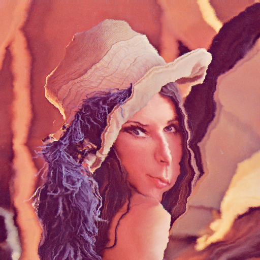
Figure 1: Two fractal homeomorphisms applied to the original picture.

The paper is organized as follows. The geometry of bi-affine functions is the subject of Section 2. Theorem 1 gives basic properties of a bi-affine function, in particular properties of the folding line and folding parabola. Theorem 2 gives a geometric construction for finding the image of a given point under a bi-affine function and precisely describes the 2-to-1 nature of a bi-affine function. Section 3 provides background on iterated function systems and their attractors. It is a classic result that, if an IFS is contractive, then it has an attractor. Theorem 3 gives fairly general conditions under which a bi-affine IFS is contractive. Fractal homeomorphism between the attractors to two IFSs is the subject of Section 4. The construction of a fractal homeomorphism depends on finding shift invariant sections of the coding maps of the two IFSs. Theorem 4 states that any such shift invariant section comes from a mask. (The terms coding map, section, shift invariant, and mask are defined in Section 4.) Theorem 5 concerns how to obtain a fractal homeomorphism between two attractors from the respective sections. The visual representation of a fractal homeomorphism for bi-affine IFSs is the subject of Section 5. Theorem 6 states that a particular type of bi-affine IFS can be used to construct fractal homeomorphisms. The main issue is proving the continuity of the map and its inverse. The pictures in Figure 1 are obtained by this method.

2 Geometry of Bi-affine Functions

Boldface letters represent vectors in ${\mathbb{R}}^{2}$. A function $f\,:\,{\mathbb{R}}^{2}\rightarrow{\mathbb{R}}^{2}$ is called bi-affine if it has the form

$$f(x,y)={\mathbf{a}}+{\mathbf{b}}x+{\mathbf{c}}y+{\mathbf{d}}xy.$$ (2 )

It is easy to verify that the class of bi-affine functions is exactly the class characterized by the two properties listed in the introduction. The class of bi-affine functions is not closed under composition, but the composition of a bi-affine and an affine function is bi-affine.

Call a bi-affine function non-degenerate if $\mathbf{d}\neq\mathbf{0}$ and neither $\mathbf{b}$ nor $\mathbf{c}$ is a scalar multiple of ${\mathbf{d}}$. In particular, neither $\mathbf{b}$ nor $\mathbf{c}$ is the zero vector. If $\mathbf{d}=0$, then $f$ is “degenerate” in the sense that it is affine and well understood. If $\mathbf{d}\neq\mathbf{0}$ and both $\mathbf{b}$ and $\mathbf{c}$ are scalar multiples of ${\mathbf{d}}$, then $f$ is “degenerate” in the sense that the range of $f$ degenerates to a line. If $\mathbf{d}\neq\mathbf{0}$ and just one of $\mathbf{b}$ and $\mathbf{c}$ is a scalar multiple of ${\mathbf{d}}$, then $f$ is “degenerate” in the sense that the image of the folding line, as defined in the next section, is just a point, a fact that can be verified by equation 4 in the proof of Theorem 1.

Basic properties of bi-affine functions are described in this section. According to statement 2 of Theorem 1 below, the image of a line $L$ under a bi-affine function is a parabola. Such a parabola can be degenerate in the sense that it is either a line (focal distance $0$) or a line that doubles back on itself (focal distance $\infty$). The first case occurs if and only if $L$ is parallel to either the $x$ or $y$-axis. An example of the second case is $(X,Y)=f(x,y)=(-x+xy,-1-y+xy)$, in which case the image of the line $y=x+1$ is given by the parametric equation $X=t^{2},\,Y=t^{2}-2$, a degenerate parabola with vertex at $(0,-2)$ that doubles back along the line $y=x-2$.

For vectors $\mathbf{a}$ and $\mathbf{b}$, let $|\mathbf{a}\;\mathbf{b}|$ denote the determinant of the matrix whose columns are $\mathbf{a}$ and $\mathbf{b}$. For a non-degenerate bi-affine functon $f$, call the line $L_{f}$ with equation

$$|\mathbf{b}\;\mathbf{d}|\,x+|\mathbf{d}\;\mathbf{c}|\,y=|\mathbf{c}\;\mathbf{b}|$$ (3 )

the folding line of the function $f$. Note that, by the non-degeneracy of $f$, neither $|\mathbf{b}\;\mathbf{d}|$ nor $|\mathbf{d}\;\mathbf{c}|$ is zero, and hence the folding line is not parallel to either the $x$ or $y$-axis. The terminology “folding line” is justified by the next theorem, in particular statement 4. The image $P_{f}=f(L_{f})$ of the folding line is called the folding parabola, which, according to statement 3 is non-degenerate. Let $L_{+}$ and $L_{-}$ denote the closed half spaces above and below $L_{f}$, respectively.

Theorem 1.

If $f$ is a non-degenerate bi-affine map, then

1. any line parallel to either coordinate axis is mapped to a line;

2. any line is mapped to a, possibly degenerate, parabola;

3. the folding parabola $P_{f}:=f(L_{f})$ is non-degenerate;

4. the map $f$ is injective when restricted to either $L_{+}$ or $L_{-}$.

Proof.

Statement (1) follows from the fact that, for a fixed $x$ or a fixed $y$, a bi-affine function is an affine function in the other variable.

The image of a line under a bi-affine transformation has a parametric equation of the form $f(t)=\mathbf{u}+\mathbf{v}\,t+\mathbf{w}\,t^{2}$, which is a, possibly degenerate, parabola.

To show that $P_{f}$ is non-degenerate, first note that the image of the line $L_{f}$ under $f$ is given by the parametric equation $(X(x),Y(x))$ with parameter $x$ by

$$(X,Y)= f(x,x)=\frac{1}{|\mathbf{d}\,\mathbf{c}|}\left[(|\mathbf{d}\,\mathbf{c}|\,\mathbf{a}+|\mathbf{c}\,\mathbf{b}|\,\mathbf{c})+(|\mathbf{d}\,\mathbf{c}|\,\mathbf{b}-|\mathbf{b}\,\mathbf{d}|\,\mathbf{c}+|\mathbf{c}\,\mathbf{b}|\,\mathbf{d})\,x+|\mathbf{b}\,\mathbf{d}|\,\mathbf{d}\,x^{2}\right]$$ (4 )

$$= \frac{1}{|\mathbf{d}\,\mathbf{c}|}\left[(|\mathbf{d}\,\mathbf{c}|\,\mathbf{a}+|\mathbf{c}\,\mathbf{b}|\,\mathbf{c})+2|\mathbf{d}\,\mathbf{b}|\,\mathbf{c}\,x+|\mathbf{b}\,\mathbf{d}|\,\mathbf{d}\,x^{2}\right],$$

the first equality simply by substituting from equation 3 into equation 2 and the second equality by a direct calculation. The tangent vector to this parabola is

$$T(x)=\frac{2\,|\mathbf{d}\,\mathbf{b}|}{|\mathbf{d}\,\mathbf{c}|}(\mathbf{c}-\mathbf{d}\,x).$$

By the non-degeneracy of $f$, the vectors $\mathbf{c}$ and $\mathbf{d}$ are linearly independent, implying that the the direction of the tangent vector is not constant. Hence the parabola is not degenerate.

The Jacobian determinant of a bi-affine function is $|\mathbf{b}\;\mathbf{d}|\,x+|\mathbf{d}\;\mathbf{c}|\,y-|\mathbf{c}\;\mathbf{b}|$, which is nonzero except on the folding line. It follows from the inverse function theorem that $f$ is injective when restricted to either $L_{+}$ or $L_{-}$. ∎

A parabola $P$ divides the plane into two regions; let $\widehat{P}$ denote the closed region “outside” P (and including $P$). The set $\widehat{P_{f}}$ will be called simply the parabolic region of $f$. For a point $\mathbf{p}=(x,y)\in{\mathbb{R}}^{2}$, let

$${\mathbf{p}}^{*}=\left(\frac{|\mathbf{c}\;\mathbf{b}|-|\mathbf{d}\;\mathbf{c}|\,y}{|\mathbf{b}\;\mathbf{d}|}\,,\,\frac{|\mathbf{c}\;\mathbf{b}|-|\mathbf{b}\;\mathbf{d}|\,x}{|\mathbf{d}\;\mathbf{c}|}\right).$$ (5 )

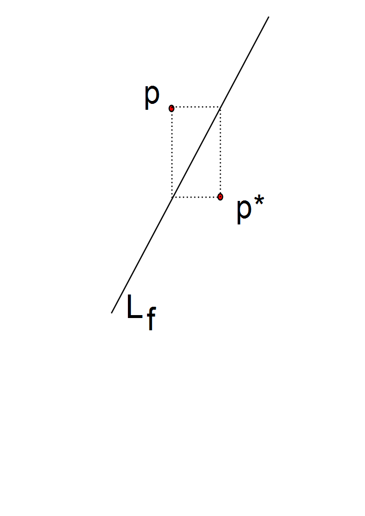
Figure 2: Folding Line $L_{f}:f({\mathbf{p}})={\mathbf{p}^{*}}$ .

This somewhat complicated formula is merely an analytic expression of the simple geometry shown in Figure 2. Statement 3 in Theorem 2 below makes precise the 2-to-1 nature of a bi-affine function given in statement 4 of Theorem 1. Statement 1 in Theorem 2 is illustrated in Figure 3. Statement 2 gives a geometric construction of the image of a given point under a bi-affine function and is illustrated in Figure 4.

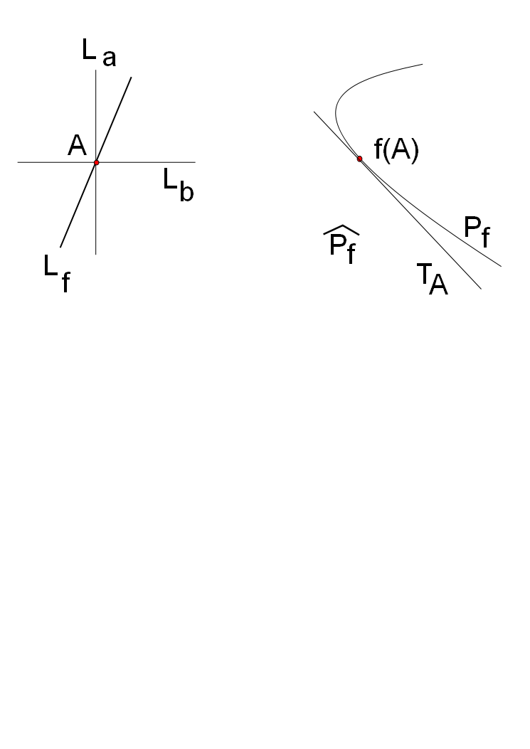
Figure 3: Folding parabola $P_{f}$, parabolic region $\widehat{P_{f}}$, tangent line $T_{A}$.

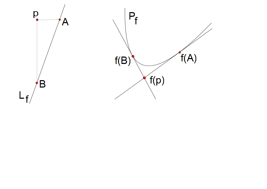
Figure 4: The image of a point $\mathbf{p}$ under a bi-affine function. The point $f(\mathbf{p})$ has “coordinates” $(A,B)$.

Theorem 2.

Assume that $f$ is a non-degenerate bi-affine map. We use the notation $L_{a}$ for the line $x=a$ and $L_{b}$ for the line $y=b$.

1. If $A=(a,b)$ is any point on the folding line $L_{f}$ and $T_{A}$ is the tangent line to $P_{f}$ at $f(A)$, then $T_{A}=f(L_{a})=f(L_{b})$.

2. If $\mathbf{p}=(a,b)\in{\mathbb{R}}^{2}$, then $f({\mathbf{p}})=T_{A}\cap T_{B}$, where $A=L_{f}\cap L_{a}$ and $B=L_{f}\cap L_{b}$.

3. $f(L_{+})=f(L_{-})=\widehat{P_{f}}$ and, in particular, $f(\mathbf{p})=f({\mathbf{p}}^{*})$ for all $\mathbf{p}=(x,y)\in{\mathbb{R}}^{2}$.

Proof.

Concerning statement 1, any horizontal or vertical line $L$ intersects $L_{f}$ in a single point. Therefore $f(L)$ intersects $f(L_{f})=P_{f}$ in a single point, which implies that $f(L)$ is tangent to $P_{f}$. Since the intersections $P_{f}\cap f(L_{a})$ and $P_{f}\cap f(L_{b}$) both consist of the same single point, $f(L_{a})$ and $f(L_{b})$ both equal the tangent line $T_{A}$ to $P_{f}$ at $f(A)$.

By statement 1, the point $f(\mathbf{p})$ lies both on the tangent to $P_{f}$ at $f(A)$ and on the tangent to $P_{f}$ at $f(B)$. This proves statement 2.

Consider $\mathbf{p}$ and $\mathbf{p}^{*}$ as in Figure 2. Statement 2 implies that $f(\mathbf{p})=T_{A}\cap T_{B}=f({\mathbf{p}}^{*})$. In particular $f(L_{+})=f(L_{-})$. Since the union of all tangents to $P_{f}$ is the parabolic region $\widehat{P_{f}}$ of $f$, we have $f(L_{+})=f(L_{-})=f({\mathbb{R}}^{2})=\widehat{P_{f}}$. ∎

It is a consequence of Theorem 2 that the parabolic region can be coordinatized as follows. Each point ${\mathbf{p}}\in\widehat{P_{f}}$ has a unique set $\{A,B\}$ of (unordered) coordinates where $A$ and $B$ are points on the folding line. Specifically $\mathbf{p}=T_{A}\cap T_{B}$. This is illustrated in Figures 4 and 5.

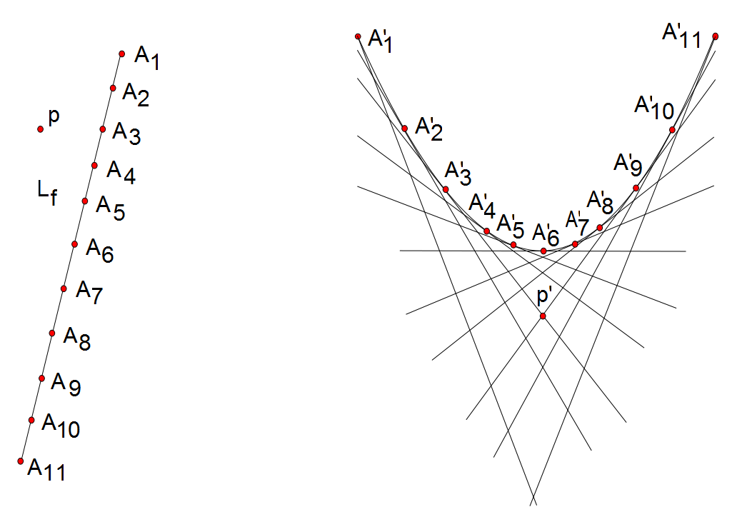
Figure 5: Coordinatization of $\widehat{P_{f}}$. Note that $A^{\prime}_{i}=f(A_{i}),\,1\leq i\leq 11,$ and ${\mathbf{p}}^{\prime}=f({\mathbf{p}})$. The point $\mathbf{p}^{\prime}$ has coordinates $\{A3,A9\}$.

The folding parabola $P_{f}$ can be constructed geometrically as follows (See Figure 6). Choose four pair wise distinct points $A_{1},A_{2},A_{3},A_{4}$ on the folding line and construct the four tangent lines $T_{A_{1}},T_{A_{2}},T_{A_{3}},T_{A_{4}}$. It is a direct consequence of the classic Brianchon Theorem (actually the converse) that there is a unique parabola with these lines as tangents. According to what has been shown above, this must be the folding parabola. The parabola can be explicitly constructed using a theorem of Lambert. According to Lambert, the circumcircle of a tangent triangle of a parabola (see Figure 6) goes through the focus of the parabola. So the focus $F$ is determined as the intersection of three such circumcircles. Then reflect $F$ about two of the tangents to get two points on the directrix.

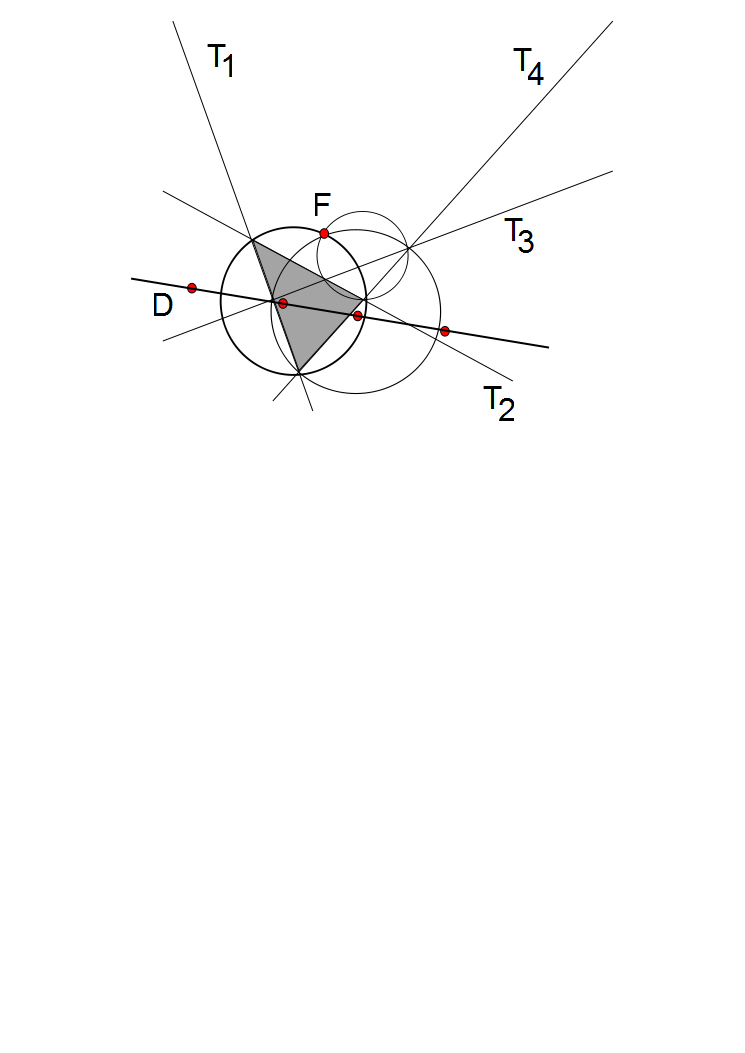
Figure 6: Construction of the folding parabola: focus $F$ and directrix $D$.

3 Iterated Function Systems

This section reviews the standard notation and definitions related to iterated function systems (IFS). These concepts are then applied to the bi-affine case.

Let $\mathbb{X}$ be a complete metric space. If $f_{m}:\mathbb{X}\rightarrow\mathbb{X}$, $m=1,2,\dots,M,$ are continuous mappings, then $\mathcal{F}=\left(\mathbb{X};f_{1},f_{2},...,f_{M}\right)$ is called an iterated function system (IFS). An iterated function system that consists of bi-affine functions will be called a bi-affine IFS. To define the attractor of an IFS, first define

$$\mathcal{F}(B)=\bigcup_{f\in\mathcal{F}}f(B)$$

for any $B\subset\mathbb{X}$. By slight abuse of terminology we use the same symbol $\mathcal{F}$ for the IFS, the set of functions in the IFS, and for the above mapping. For $B\subset\mathbb{X}$, let $\mathcal{F}^{k}(B)$ denote the $k$-fold composition of $\mathcal{F}$, the union of $f_{i_{1}}\circ f_{i_{2}}\circ\cdots\circ f_{i_{k}}(B)$ over all finite words $i_{1}i_{2}\cdots i_{k}$ of length $k.$ Define $\mathcal{F}^{0}(B)=B.$ A nonempty compact set $A\subset\mathbb{X}$ is said to be an attractor of the IFS $\mathcal{F}$ if

1. $\mathcal{F}(A)=A$ and

2. $\lim_{k\rightarrow\infty}\mathcal{F}^{k}(B)=A,$ for all compact sets $B\subset\mathbb{X}$, where the limit is with respect to the Hausdorff metric.

Attractors for bi-affine IFSs consisting, respectively of $2,3$ and $4$, functions are shown in Figure 7.

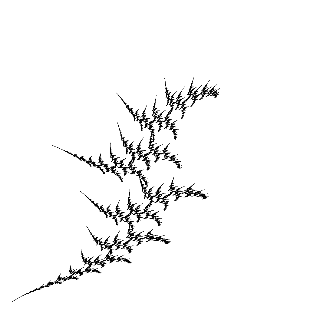
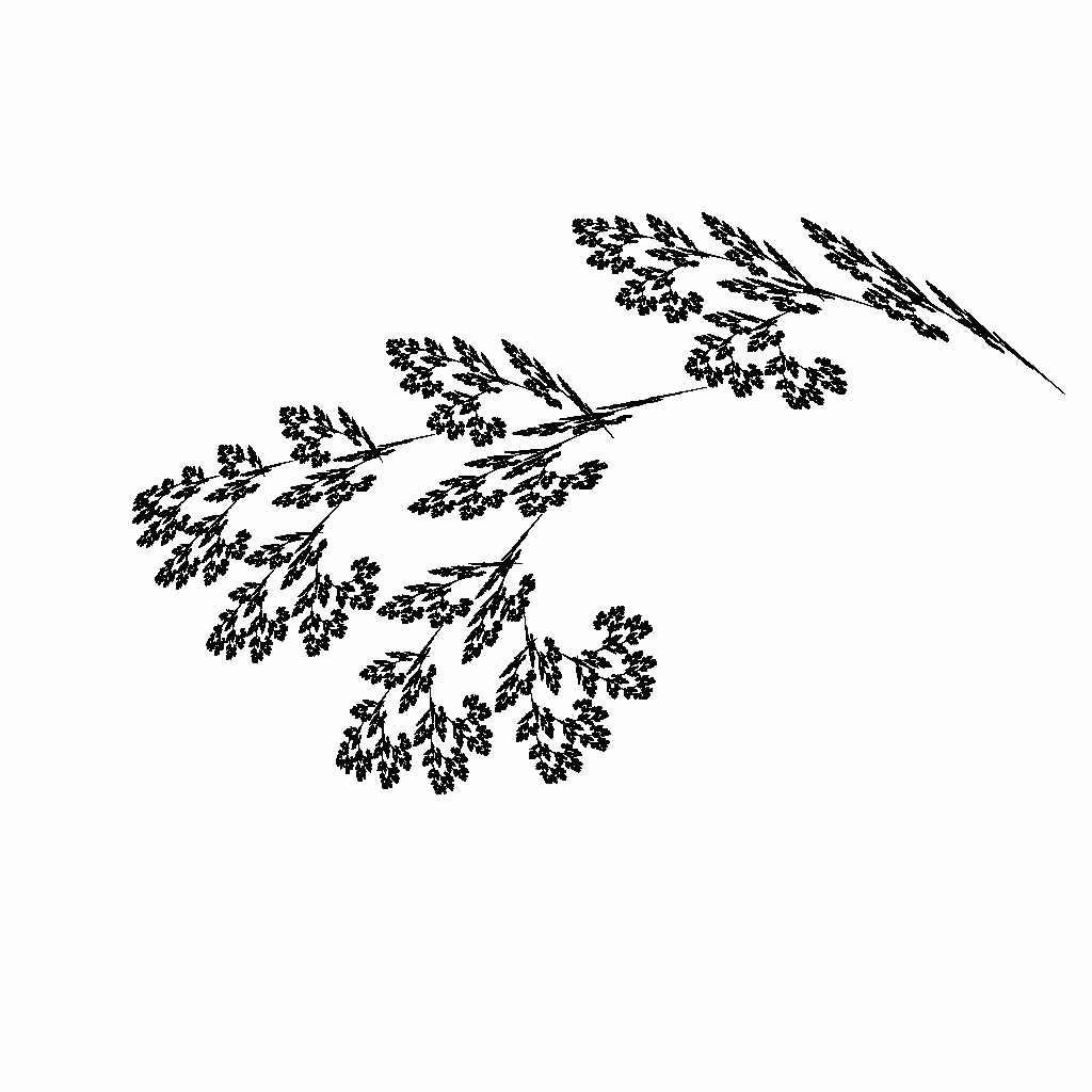
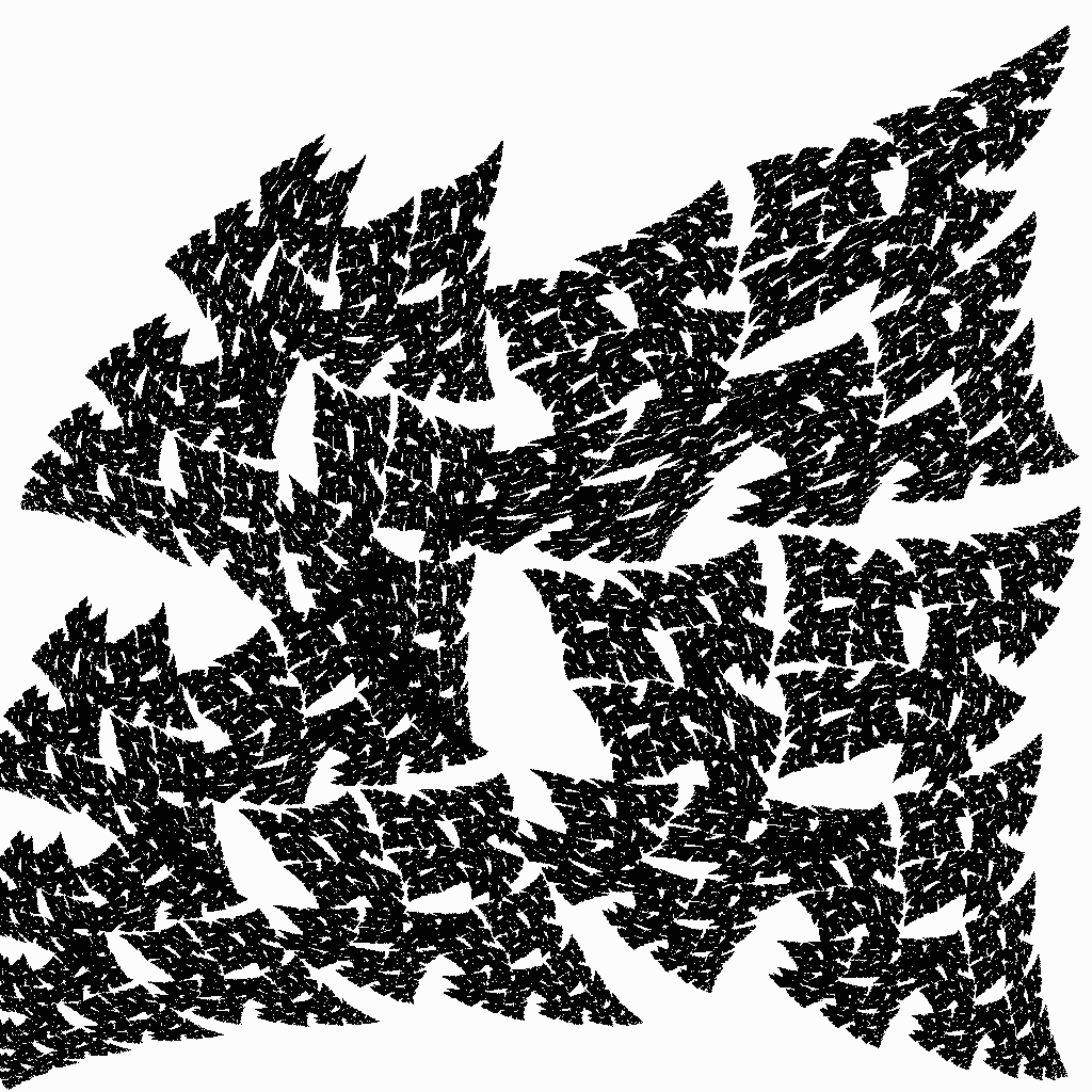
Figure 7: Attractors of IFSs consisting of two, three, and four bi-affine functions, respectively.

A function $f:\mathbb{X}\rightarrow\mathbb{X}$ is called a contraction with respect to a metric $d$ if there is an $0\leq s<1$ such that $d(f(x),f(y))\leq s\,d(x,y)$ for all $x,y\in{\mathbb{R}}^{n}$. An IFS with the property that each function is a contraction will be called a contractive IFS. In his seminal paper Hutchinson [4] proved that a contractive IFS on a complete metric space has a unique attractor. Theorem 3 below gives fairly general conditions under which a bi-affine IFS is contractive.

Let       denote the unit square with vertices $(0,0),(1,0),(1,1),(0,1)$. The shape of the image of       under a non-degenerate bi-affine map $f$ depends on the location of the folding line $L_{f}$ relative to       . It follows from Theorem 2 that there are three possible cases as shown in Figure 8. It is only in Case 1 ($L_{f}$ disjoint from the interior of       ) that the image of the sides of       form a convex quadrilateral. If this is the case, call $f$ proper.

Note that the unique bi-affine function taking $(0,0),(1,0),(1,1),(0,1)$ to the points $\mathbf{p}_{0},\mathbf{p}_{1},\mathbf{p}_{2},\mathbf{p}_{3}$, respectively, is

$$f(x,y)=\mathbf{p}_{0}+(\mathbf{p}_{1}-\mathbf{p}_{0})x+(\mathbf{p}_{3}-\mathbf{p}_{0})y+(\mathbf{p}_{2}+\mathbf{p}_{0}-\mathbf{p}_{1}-\mathbf{p}_{3})xy.$$ (6 )

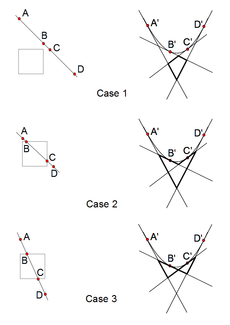
Figure 8: The image of the sides of the unit square (on the left) is shown by thick lines (on the right): $A^{\prime}=f(A),\,B^{\prime}=f(B),\,C^{\prime}=f(C),\,D^{\prime}=f(D)$.

Theorem 3.

Let $f(x,y)=\mathbf{p}_{0}+(\mathbf{p}_{1}-\mathbf{p}_{0})x+(\mathbf{p}_{3}-\mathbf{p}_{0})y+(\mathbf{p}_{2}+\mathbf{p}_{0}-\mathbf{p}_{1}-\mathbf{p}_{3})xy$ be a proper, non-degenerate bi-affine function. If there is an $s,\,0\leq s<1$, such that

$$|\mathbf{p}_{i+1}-\mathbf{p}_{i}|\leq s,\quad|\mathbf{p}_{i+2}-\mathbf{p}_{i}|\leq\sqrt{2}s,\quad|\mathbf{p}_{i+1}+\mathbf{p}_{i-1}-2\mathbf{p}_{i}|\leq\sqrt{2}s$$

for $i=0,1,2,3\;(mod\;4)$, then $f$ is a contraction on       .

In terms of the quadrilateral $\mathbf{p}_{0}\mathbf{p}_{1}\mathbf{p}_{2}\mathbf{p}_{3}$, the first of the three inequalities states that each side has length less than or equal to $s$, the second that each diagonal has length less than or equal to $\sqrt{2}s$, and the third that vector sum of any two incident sides has length less or equal to $\sqrt{2}s$. For a bi-affine function taking       into itself, for example, these conditions are not too restrictive. Two lemmas help in proving Theorem 3.

Lemma 1.

If $f$ is a proper, non-degenerate bi-affine function, then $f$ is injective when restricted to       .

Proof.

By the comments above, the folding line $L_{f}$ lies outside the interior of the square       . The lemma then follows by statement 4 of Theorem 1. ∎

Lemma 2.

Let $f$ be a non-degenerate bi-affine function that is injective on       , and let $W\subseteq\mathchoice{\vbox{\vbox{\hrule height=0.8pt\hbox{\vrule width=0.8pt,height=6.0pt\kern 6.0pt\vrule width=0.8pt} \hrule height=0.8pt}}}{\vbox{\vbox{\hrule height=0.8pt\hbox{\vrule width=0.8pt,height=6.0pt\kern 6.0pt\vrule width=0.8pt} \hrule height=0.8pt}}}{\vbox{\vbox{\hrule height=0.3pt\hbox{\vrule width=0.3pt,height=2.1pt\kern 2.1pt\vrule width=0.3pt} \hrule height=0.3pt}}}{\vbox{\vbox{\hrule height=0.3pt\hbox{\vrule width=0.3pt,height=1.5pt\kern 1.5pt\vrule width=0.3pt} \hrule height=0.3pt}}}$ be any rectangle with sides parallel to the $x$ and $y$-axes and with diagonal of length $\rho(W)$. Further let $\rho_{1}(W)$ and $\rho_{2}(W)$ be the lengths of the two diagonals of $f(W)$ and let

$$M(\rho_{0})=\max_{W:\rho(W)=\rho_{0}}\max(\rho_{1}(W),\rho_{2}(W)).$$

For any $\rho_{0}\leq\sqrt{2}$, if $W_{0}$ is a rectangle that maximizes $M(\rho_{0})$, then $W_{0}$ and       have a common vertex.

Proof.

If one side of $W_{0}$ lies on the line $x=0$ or $x=1$ and another side lies on $y=0$ or $y=1$, then the proof is complete. So, without loss of generality, assume that $W_{0}$ has no side that lies on $x=0$ or $x=1$. Let $V_{0}$ be the rectangle bounded by the lines $x=0,x=1$ and the lines determined by the upper and lower sides of $W_{0}$. Let $A,B,C,D$ be the vertices of $f(V_{0})$. Then by the conditions 1 in the Introduction, there is an $\alpha$ such that the four vertices of $f(W_{0})$ are $(1-\alpha)A+\alpha B,(1-\alpha-\Delta)A+(\alpha+\Delta)B,(1-\alpha-\Delta)C+(\alpha+\Delta)D,(1-\alpha)D+\alpha C$, where $\Delta$ is the horizontal length of $W_{0}$. As $\alpha$ varies between $0$ and $\alpha_{0}$, the rectangle $W_{0}$ shifts left or right, from the extreme left side of       to the extreme right side of       . The lengths of the two diagonals of $f(W_{0})$ are $|U_{1}+(B+C-A-D)\alpha|$ and $|U_{2}+(B+C-A-D)\alpha|$, where vectors $U_{1}$ and $U_{2}$ depend on $A,B,C,D$ and $\Delta$. As $\alpha$ varies in the range $0\leq\alpha\leq\alpha_{0}$, the quantities $U_{1}+(B+C-A-D)\alpha$ and $U_{2}+(B+C-A-D)\alpha$ describe (parallel) line segments. Hence the maximum of $|U_{1}+(B+C-A-D)\alpha|$ and $|U_{2}+(B+C-A-D)\alpha|$ occur at an end, i.e. $\alpha=0$ or $\alpha=\alpha_{0}$, contradicting the assumption that $W_{0}$ has no side that lies on $x=0$ or $x=1$. ∎

Proof.

(of Theorem 3) By the continuity of $f$ and the compactness of       , it is sufficient to show that there is an $s,\,0\leq s<1$ such that $|f(x,y)-f(x^{\prime},y^{\prime})|\leq s\,|(x,y)-(x^{\prime},y^{\prime})|$. Let $W_{0}$ be the rectangle whose diagonal is the line segment joining $(x,y)$ and $(x^{\prime}y^{\prime})$. By Lemma 1, the function $f$ is injective on       , and by Lemma 2, the quantity

$$R:=\frac{|f(x,y)-f(x^{\prime},y^{\prime})|}{|(x,y)-(x^{\prime},y^{\prime})|},\,(x,y)\neq(x^{\prime},y^{\prime})$$

is maximized when $W_{0}$ and       have a common vertex, i.e. when $W_{0}$ lies on the corner of       . Without loss of generality, it may be assumed to be the lower left corner. Otherwise, replace $f$ with the composition of $f$ with the rotation that moves the lower left corner to the relevant corner. Now let $\Delta x=|x^{\prime}-x|$ and $\Delta y=|y^{\prime}-y|$. With $\mathbf{b}=\mathbf{p}_{1}-\mathbf{p}_{0},\mathbf{c}=\mathbf{p}_{3}-\mathbf{p}_{0},\mathbf{d}=\mathbf{p}_{2}+\mathbf{p}_{0}-\mathbf{p}_{1}-\mathbf{p}_{3}$ and setting $r=\frac{\Delta y}{\Delta x}$, we have two possible formulas for $R$:

$$R^{2}=\frac{|f(\Delta x,\Delta y)-f(0,0)|^{2}}{\Delta x,\Delta y)|^{2}}=\frac{1}{1+r^{2}}|\mathbf{b}+r\mathbf{c}\ +r\Delta x\mathbf{d}|^{2}$$

or

$$R^{2}=\frac{|f(\Delta x,0)-f(0,\Delta y)|^{2}}{\Delta x,\Delta y)|^{2}}=\frac{1}{1+r^{2}}|\mathbf{b}-r\mathbf{c}|^{2}.$$

Since $0<\Delta x\leq 1$, the quantity $R^{2}$ in the first formula is maximized when either $\Delta x=0$ or $\Delta x=1$. So it is now sufficient to prove that

$$\max_{r>0}\,\big{(}\frac{1}{1+r^{2}}|\mathbf{b}+r\mathbf{c}|^{2},\,\frac{1}{1+r^{2}}|\mathbf{b}+r\mathbf{c}+r\mathbf{d}|^{2},\,\frac{1}{1+r^{2}}|\mathbf{b}-r\mathbf{c}|^{2}\big{)}<1.$$

The inequalities in the statement of the theorem, in terms of $\mathbf{b},\mathbf{c},\mathbf{d}$ are that $|\mathbf{b}|,|\mathbf{c}|,|\mathbf{b}+\mathbf{d}|,|\mathbf{c}+\mathbf{d}|$ are all less than or equal to $s$ and $|\mathbf{b}-\mathbf{c}|,|\mathbf{b}+\mathbf{c}+\mathbf{d}|,|\mathbf{b}+\mathbf{c}|,|\mathbf{b}-\mathbf{c}+\mathbf{d}|,|\mathbf{c}-\mathbf{b}+\mathbf{d}|,|\mathbf{b}+\mathbf{c}+2\mathbf{d}|$ are all less than or equal to $\sqrt{2}s$. Maximizing the three quantities over $r$, in order to verify the above inequality, is a not quite trivial calculus problem whose details are omitted. ∎

Example 1.

Consider a bi-affine IFS ${\mathcal{F}}=\{\mathchoice{\vbox{\vbox{\hrule height=0.8pt\hbox{\vrule width=0.8pt,height=6.0pt\kern 6.0pt\vrule width=0.8pt} \hrule height=0.8pt}}}{\vbox{\vbox{\hrule height=0.8pt\hbox{\vrule width=0.8pt,height=6.0pt\kern 6.0pt\vrule width=0.8pt} \hrule height=0.8pt}}}{\vbox{\vbox{\hrule height=0.3pt\hbox{\vrule width=0.3pt,height=2.1pt\kern 2.1pt\vrule width=0.3pt} \hrule height=0.3pt}}}{\vbox{\vbox{\hrule height=0.3pt\hbox{\vrule width=0.3pt,height=1.5pt\kern 1.5pt\vrule width=0.3pt} \hrule height=0.3pt}}}\,;\,f_{1},f_{2},f_{3},f_{4}\}$, where the four functions are determined by the images of the four vertices of       as shown in Figure 9. Each of the four images $f_{i}(\mathchoice{\vbox{\vbox{\hrule height=0.8pt\hbox{\vrule width=0.8pt,height=6.0pt\kern 6.0pt\vrule width=0.8pt} \hrule height=0.8pt}}}{\vbox{\vbox{\hrule height=0.8pt\hbox{\vrule width=0.8pt,height=6.0pt\kern 6.0pt\vrule width=0.8pt} \hrule height=0.8pt}}}{\vbox{\vbox{\hrule height=0.3pt\hbox{\vrule width=0.3pt,height=2.1pt\kern 2.1pt\vrule width=0.3pt} \hrule height=0.3pt}}}{\vbox{\vbox{\hrule height=0.3pt\hbox{\vrule width=0.3pt,height=1.5pt\kern 1.5pt\vrule width=0.3pt} \hrule height=0.3pt}}}),\,i=1,2,3,4$, of the square contains exactly one vertex of       . The attractor of ${\mathcal{F}}$ is       itself. For “most” choices of the center and side points, ${\mathcal{F}}$ satisfies the conditions of Theorem 3 and hence ${\mathcal{F}}$ is a contractive IFS. Why this simple example should be of interest is the subject of the next two sections.

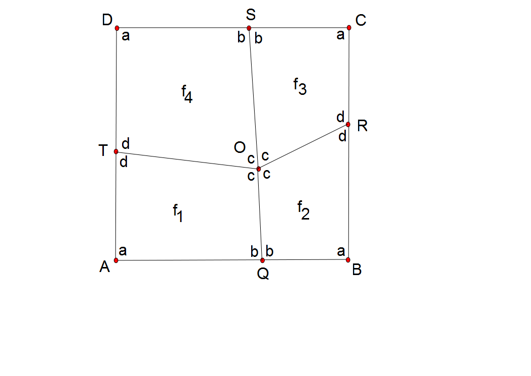
Figure 9: An IFS consists of four bi-affine functions. Points labeled with lower case letters are the images of points labeled with upper case letters. The attractor is the unit square.

4 Fractal Homeomorphism

In the case of a contractive IFS, it is possible to assign to each point of the attractor an “address”. Given two IFSs ${\mathcal{F}}$ and ${\mathcal{G}}$ with respective attractors $A_{F}$ and $A_{G}$, a fractal homeomorphism is basically a homeomorphism $h\,:\,A_{F}\rightarrow A_{G}$ that sends a point in $A_{F}$ to the point in $A_{G}$ with the same address. To make this notion precise, let $\mathcal{F}=\left(\mathbb{X};f_{1},f_{2},...,f_{N}\right)$ be a contractive IFSs on a complete metric space $\mathbb{X}$ with attractor $A$. Let $\Omega=\{1,2,\dots,N\}^{\infty}$ denote the set of infinite strings using symbols $1,2,\dots,N$, and for $\sigma\in\Omega$, let $\sigma|_{k}$ denote the string consisting of the first $k$ symbols in $\sigma$. Moreover, if $\sigma=i_{0}\,i_{1},\,i_{2}\cdots$, then we use the notation

$$f_{\sigma|_{n}}:=f_{i_{0}}\circ f_{i_{1}}\circ\cdots\circ f_{i_{n}}.$$

Now define a map $\pi:\Omega\rightarrow A$, called the coding map, by

$$\pi(\sigma):=\lim_{k\rightarrow\infty}f_{\sigma|_{k}}(x).$$

It is well known [1, 4] that the limit above exists and is independent of $x\in\mathbb{X}$. Moreover $\pi$ is continuous, onto, and satisfies the following commuting diagram for each $n=1,2,\dots,N$.

$$\begin{array}[c]{ccc}\Omega&\overset{s_{n}}{\rightarrow}&\Omega\\ \pi\downarrow\text{\ \ \ \ }&&\text{ \ \ \ }\downarrow\pi\\ \mathbb{X}&\underset{f_{n}}{\rightarrow}&\mathbb{X}\end{array}$$ (7 )

The symbol $s_{n}:\Omega\rightarrow\Omega$ denotes the inverse shift map defined by $s_{n}(\sigma)=n\sigma.$ A section of the coding map $\pi$ is a function $\tau\,:\,\Omega\rightarrow A$ such that $\pi\circ\tau$ is the identity. A section selects, for each $x\in A$, a single address in $\Omega$ from the ones that come from the coding map. Call the set $\Omega_{\tau}:=\tau(A)$ the address space of the section $\tau$. Let $S$ denote the shift operator on $\Omega$, i.e, $S(n\sigma)=\sigma$ for any $n\in\{1,2,\dots,N\}$ and any $\sigma\in\Omega$. A subset $W\subset\Omega$ will be called shift invariant if $\sigma\in W$ implies that $S(\sigma)\in W$. If $\Omega_{\tau}$ is shift invariant, then $\tau$ is called a shift invariant section. The following example demonstrates the naturalness of shift invariant sections.

Example 2.

Consider the IFS ${\mathcal{F}}=({\mathbb{R}}\,;\,f_{0},f_{1})$ where $f_{0}(x)=\frac{1}{2}\,x$ and $f_{1}(x)=\frac{1}{2}\,x+\frac{1}{2}$. The attractor is the interval $[0,1]$. An address of a point $x$ is a binary representation of $x$. In choosing a section $\tau$ one must decide, for example, whether to take $\tau(\frac{1}{4})=.01$ or $\tau(\frac{1}{4})=.00111\cdots$. If the section $\tau$ is shift invariant, this would imply, for example, that if $\tau(\frac{1}{4})=.00111\cdots$, then $\tau(\frac{1}{2})=.0111\cdots$, not $\tau(\frac{1}{2})=.100\cdots$.

Lemma 3.

With notation as above, a section $\tau$ of an IFS is shift invariant if and only if, for any $x\in A$, if $\tau(x)|_{1}=n$, then $(S\circ\tau)(x)=(\tau\circ f^{-1}_{n})(x)$.

Proof.

Given the right hand statement above, we will prove that $\tau$ is shift invariant. Assume that $n\sigma\in\Omega_{\tau}$. Then there is an $x\in A$ such that $\tau(x)=n\sigma$, and hence $\sigma=(S\circ\tau)(x)=(\tau\circ f^{-1}_{n})(x)=\tau(f^{-1}_{n})(x))$. Thus $\sigma\in\Omega_{\tau}$.

Conversely, assume that $\tau$ is shift invariant. Assume that $x\in A$ and $\tau(x)=n\sigma$ for some $\sigma\in\Omega$. By shift invariance, there is a $y\in A$ such that $\tau(y)=\sigma$. Now

$$x=(\pi\circ\tau)(x)=\pi(n\sigma)=f_{n}(\lim_{k\rightarrow\infty}f_{\sigma|_{k}}(A))=f_{n}(\pi(\tau(y)))=f_{n}(y).$$

Therefore $y=f_{n}^{-1}(x)$ and

$$(S\circ\tau)(x)=S(n\sigma)=\sigma=\tau(y)=\tau(r_{n}^{-1}(x))=(\tau\circ f^{-1}_{n})(x).$$

∎

Call an IFS injective if each function in the IFS is injective. Theorem 4 below states that every shift invariant section of an injective IFS can be obtained from a mask. For an IFS $\mathcal{F}$ with attractor $A$, a mask is a partition $M=\{M_{i},1\leq i\leq N\}$ of $A$ such that $M_{i}\subseteq f_{i}(A)$ for all $f_{i}\in{\mathcal{F}}$. Given an injective IFS $\mathcal{F}$ and a mask $M$, consider the function $T\,:\,A\rightarrow A$ defined by $T(x):=f_{i}^{-1}(x)$ when $x\in M_{i}$. The itinerary $\tau_{M}(x)$ of a point $x\in A$ is the string $i_{0}\,i_{1}\,i_{2}\cdots\in\Omega$, where $i_{k}$ is the unique integer $1\leq i_{k}\leq N$ such that

$$T^{k}(x)\in M_{i_{k}}.$$

Theorem 4.

Let $\mathcal{F}$ be a contractive and injective IFS.

1. If $M$ is a mask, then $\tau_{M}$ is a shift invariant section of $\pi$.

2. If $\tau$ is a shift invariant section of $\pi$, then $\tau=\tau_{M}$ for some mask $M$.

Proof.

To show that $\tau_{M}$ is a section, let $x\in A$. Then $(\pi\circ\tau_{M})(x)=\lim_{k\rightarrow\infty}f_{\tau_{M}(x)|_{k}}(A)$. It follows immediately from the definition of $\tau_{M}$ that $x\in f_{\tau_{M}(x)|_{k}}(M_{i_{k+1}})\subseteq f_{\tau_{M}(x)|_{k}}(A)$ for all $k$. Hence $(\pi\circ\tau_{M})(x)=x$. Concerning the shift invariance, it follows from the definition of $T$ that the following diagram commutes.

$$\begin{array}[c]{ccc}A&\overset{T}{\rightarrow}&A\\ \tau_{M}\downarrow\text{\ \ \ \ }&&\text{ \ \ \ }\downarrow\tau_{M}\\ \Omega&\underset{S}{\rightarrow}&\Omega\end{array}$$ (8 )

If $\sigma\in\Omega_{\tau_{M}}$, then there is an $x\in A$ such that $\sigma=\tau_{M}(x)$ and, from the diagram, $S(\sigma)=(S\circ\tau_{M})(x)=(\tau_{M}\circ T)(x)=\tau_{M}(f_{n}^{-1}(x))\in\Omega_{\tau_{M}}$ for some $n\in\{1,2,\dots,N\}$.

Concerning the second statement, define a mask $M=\{M_{i},1\leq i\leq N\}$ as follows:

$$M_{i}=\{x\,:\,\tau(x)=i\,\sigma\quad\text{for some}\quad\sigma\in\Omega\}.$$

It is sufficient to show that $M_{i}\subseteq f_{i}(A)$, and that $\tau_{M}(x)=\tau(x)$ for all $x\in A$. If $x\in M_{i}$, then $\tau(x)=i\sigma$ for some $\sigma\in\Omega$ and $x=(\pi\circ\tau)(x)=f_{i}(\lim_{k\rightarrow\infty}f_{\sigma|_{k}}(A))\in f_{i}(A)$.

To show that $\tau_{M}(x)=\tau(x)$, let $\tau(x)=j_{0}j_{1}j_{2}\cdots$ and $\tau_{M}(x)=k_{0}k_{1}k_{2}\cdots$. That $j_{0}=k_{0}$ follows form the definitions. By induction, assume that $j_{i}=k_{i}\,i=0,1,\dots,m-1$. Applying Lemma 3 for $m$ times yields

$$j_{m}=(S^{m}\circ\tau)(x))|_{1}=\tau(f_{j_{m-1}}^{-1}\circ\cdots\circ f_{j_{1}}^{-1}\circ f_{j_{0}}^{-1}(x)|_{1},$$

where the $j_{i}$’s are determined by the recursive formula $\tau(f_{j_{r-1}}^{-1}\circ\cdots\circ f_{j_{1}}^{-1}\circ f_{j_{0}}^{-1}(x)|_{1}=j_{r}$. By the definition of the mask, $\tau(f_{j_{m-1}}^{-1}\circ\cdots\circ f_{j_{1}}^{-1}\circ f_{k_{0}}^{-1}(x))\in M_{j_{m}}$. But by the definition of the itinerary, the $k_{i}$’s are determined by the recursive formula

$$\tau(f_{k_{r-1}}^{-1}\circ\cdots\circ f_{k_{1}}^{-1}\circ f_{k_{0}}^{-1}(x))\in M_{k_{r}}$$

for $r=0,1,2,\dots,m$. But, since $k_{i}=j_{i}\,i=0,1,\dots,m-1$, we have $\tau(f_{j_{m-1}}^{-1}\circ\cdots\circ f_{j_{1}}^{-1}\circ f_{j_{0}}^{-1}(x))\in M_{k_{m}}.$ Therefore $k_{m}=j_{m}$. ∎

To define fractal homeomorphism, consider two contractive IFSs $\mathcal{F}=\left(\mathbb{X};f_{1},f_{2},...,f_{N}\right)$ and $\mathcal{G}=\left(\mathbb{X};g_{1},g_{2},...,g_{N}\right)$ with the same number $N$ of functions on a complete metric space $\mathbb{X}$. Let $A_{F}$ and $A_{G}$ be the attractors and $\pi_{F}$ and $\pi_{G}$ the coding maps of $\mathcal{F}$ and $\mathcal{G}$, respectively. A homeomorphism $h\,:\,A_{F}\rightarrow A_{G}$ is called a fractal homeomorphism if there exist shift invariant sections $\tau_{F}$ and $\tau_{G}$ such that the following diagram commutes:

$$\begin{array}[c]{ccc}A_{F}&\underset{h}{\rightarrow}&A_{G}\\ \text{$\tau_{F}$}\searrow&&\swarrow\text{$\tau_{G}$}\\ &\Omega&\end{array}$$ (9 )

i.e., the homeomorphism $h$ takes each point $x\in A_{F}$ with address $\sigma=\tau_{F}(x)$ to the point $y\in A_{G}$ with the same address $\sigma=\tau_{G}(y)$. Theorem 5 below states that the fractal homeomorphisms between attractors $A_{F}$ and $A_{G}$ are exactly mappings of the form $\pi_{G}\circ\tau_{F}$ or $\pi_{F}\circ\tau_{G}$ for some shift invariant sections $\tau_{F},\,\tau_{G}$.

Theorem 5.

Let $\mathcal{F}$ and $\mathcal{G}$ be contractive IFSs. With notation as above:

1. If $h\,:\,A_{F}\rightarrow A_{G}$ is a fractal homeomorphism with corresponding sections $\tau_{F}$ and $\tau_{G}$, then $\Omega_{\tau_{F}}=\Omega_{\tau_{G}}$. Moreover $h=\pi_{G}\circ\tau_{F}$ and $h^{-1}=\pi_{F}\circ\tau_{G}$ .

2. If $\tau_{F}$ is a shift invariant section for $\mathcal{F}$ and $h:=\pi_{G}\circ\tau_{F}$ is a homeomorphism, then $h$ is a fractal homeomorphism.

Proof.

Concerning statement 1, since $h$ is a bijection, the commuting diagram 9 implies that the images of $\tau_{F}$ and $\tau_{G}$ are equal, i.e., $\Omega_{\tau_{F}}=\Omega_{\tau_{G}}$. Now $\tau_{F}=\tau_{G}\circ h$ from the diagram implies $\pi_{G}\circ\tau_{F}=\pi_{G}\circ\tau_{F}=(\pi_{G}\circ\tau_{G})\circ h=h$. The formula involving $h^{-1}$ is likewise proved.

Concerning statement 2, the section $\tau_{F}$ is a bijection from $A_{F}$ onto $\Omega_{\tau_{F}}$. Since $h$ is also a bijection, the equality $h=\pi_{G}\circ\tau_{F}$ implies that $\pi_{G}|_{\Omega_{F}}$, the restriction of $\pi_{G}$ to $\Omega_{F}$, is a bijection onto $A_{G}$. If $\tau_{G}$ is the inverse of $\pi_{G}|_{\Omega_{F}}$, then $\tau_{F}$ and $\tau_{G}$ satisfy the commuting diagram 9. That $\tau_{F}$ is shift invariant means that $\Omega_{\tau_{G}}=\Omega_{\tau_{F}}$ , i.e., $\tau_{G}$ is shift invariant. ∎

5 Image from a Fractal Homeomorphism

This section concerns images on the unit square       . Define an image as a function $c\,:\,\mathchoice{\vbox{\vbox{\hrule height=0.8pt\hbox{\vrule width=0.8pt,height=6.0pt\kern 6.0pt\vrule width=0.8pt} \hrule height=0.8pt}}}{\vbox{\vbox{\hrule height=0.8pt\hbox{\vrule width=0.8pt,height=6.0pt\kern 6.0pt\vrule width=0.8pt} \hrule height=0.8pt}}}{\vbox{\vbox{\hrule height=0.3pt\hbox{\vrule width=0.3pt,height=2.1pt\kern 2.1pt\vrule width=0.3pt} \hrule height=0.3pt}}}{\vbox{\vbox{\hrule height=0.3pt\hbox{\vrule width=0.3pt,height=1.5pt\kern 1.5pt\vrule width=0.3pt} \hrule height=0.3pt}}}\rightarrow{\cal C}$, where $\cal C$ denotes the color palate, for example ${\cal C}=\{0,1,2,\dots,255\}^{3}$. If $h$ is any homeomorphism from       onto       , define the transformed image $h(c)\,:\,\mathchoice{\vbox{\vbox{\hrule height=0.8pt\hbox{\vrule width=0.8pt,height=6.0pt\kern 6.0pt\vrule width=0.8pt} \hrule height=0.8pt}}}{\vbox{\vbox{\hrule height=0.8pt\hbox{\vrule width=0.8pt,height=6.0pt\kern 6.0pt\vrule width=0.8pt} \hrule height=0.8pt}}}{\vbox{\vbox{\hrule height=0.3pt\hbox{\vrule width=0.3pt,height=2.1pt\kern 2.1pt\vrule width=0.3pt} \hrule height=0.3pt}}}{\vbox{\vbox{\hrule height=0.3pt\hbox{\vrule width=0.3pt,height=1.5pt\kern 1.5pt\vrule width=0.3pt} \hrule height=0.3pt}}}\rightarrow{\cal C}$ by

$$h(c):=c\circ h.$$

We are interested in the case where $h$ is a fractal homeomorphism. The remainder of this section concerns fractal homeomorphism based on bi-affine IFSs with four functions as described in Example 1.

Consider Example 1 depicted in Figure 9. For the bi-affine IFS ${\mathcal{F}}=\{\mathchoice{\vbox{\vbox{\hrule height=0.8pt\hbox{\vrule width=0.8pt,height=6.0pt\kern 6.0pt\vrule width=0.8pt} \hrule height=0.8pt}}}{\vbox{\vbox{\hrule height=0.8pt\hbox{\vrule width=0.8pt,height=6.0pt\kern 6.0pt\vrule width=0.8pt} \hrule height=0.8pt}}}{\vbox{\vbox{\hrule height=0.3pt\hbox{\vrule width=0.3pt,height=2.1pt\kern 2.1pt\vrule width=0.3pt} \hrule height=0.3pt}}}{\vbox{\vbox{\hrule height=0.3pt\hbox{\vrule width=0.3pt,height=1.5pt\kern 1.5pt\vrule width=0.3pt} \hrule height=0.3pt}}}\,;\,f_{1},f_{2},f_{3},f_{4}\}$, we will construct a section $\tau_{F}$ that is referred to in [2] as the top section. Consider the mask $M_{F}=\{M_{1},M_{2},M_{3},M_{4}\}$ defined recursively by

$$M_{i}=f_{i}(\mathchoice{\vbox{\vbox{\hrule height=0.8pt\hbox{\vrule width=0.8pt,height=6.0pt\kern 6.0pt\vrule width=0.8pt} \hrule height=0.8pt}}}{\vbox{\vbox{\hrule height=0.8pt\hbox{\vrule width=0.8pt,height=6.0pt\kern 6.0pt\vrule width=0.8pt} \hrule height=0.8pt}}}{\vbox{\vbox{\hrule height=0.3pt\hbox{\vrule width=0.3pt,height=2.1pt\kern 2.1pt\vrule width=0.3pt} \hrule height=0.3pt}}}{\vbox{\vbox{\hrule height=0.3pt\hbox{\vrule width=0.3pt,height=1.5pt\kern 1.5pt\vrule width=0.3pt} \hrule height=0.3pt}}})\setminus\bigcup_{j=1}^{i-1}f_{j}(\mathchoice{\vbox{\vbox{\hrule height=0.8pt\hbox{\vrule width=0.8pt,height=6.0pt\kern 6.0pt\vrule width=0.8pt} \hrule height=0.8pt}}}{\vbox{\vbox{\hrule height=0.8pt\hbox{\vrule width=0.8pt,height=6.0pt\kern 6.0pt\vrule width=0.8pt} \hrule height=0.8pt}}}{\vbox{\vbox{\hrule height=0.3pt\hbox{\vrule width=0.3pt,height=2.1pt\kern 2.1pt\vrule width=0.3pt} \hrule height=0.3pt}}}{\vbox{\vbox{\hrule height=0.3pt\hbox{\vrule width=0.3pt,height=1.5pt\kern 1.5pt\vrule width=0.3pt} \hrule height=0.3pt}}})$$

for $i=1,2,3,4$. Explicitly, $M_{1}$ is the closed quadrilateral $ATOQ$, $M_{2}$ is the open quadrilateral $OQBR$ together with the segments $(Q,B],[B,R],[R,O)$, $M_{3}$ is the open quadrilateral $ORCS$ together with the segments $(R,C],[C,S],[S,O)$, and $M_{4}$ is the open quadrilateral $OSDT$ together with the segments $(S,D],[D,T)$. The section $\tau_{F}$ corresponding to the mask $M_{F}$ is given by $\tau(x)=\max\pi^{-1}(x)$, where the maximum is with respect to the lexicographic order on $\Omega$.

Now consider a second bi-affine IFS ${\mathcal{G}}=\{\mathchoice{\vbox{\vbox{\hrule height=0.8pt\hbox{\vrule width=0.8pt,height=6.0pt\kern 6.0pt\vrule width=0.8pt} \hrule height=0.8pt}}}{\vbox{\vbox{\hrule height=0.8pt\hbox{\vrule width=0.8pt,height=6.0pt\kern 6.0pt\vrule width=0.8pt} \hrule height=0.8pt}}}{\vbox{\vbox{\hrule height=0.3pt\hbox{\vrule width=0.3pt,height=2.1pt\kern 2.1pt\vrule width=0.3pt} \hrule height=0.3pt}}}{\vbox{\vbox{\hrule height=0.3pt\hbox{\vrule width=0.3pt,height=1.5pt\kern 1.5pt\vrule width=0.3pt} \hrule height=0.3pt}}}\,;\,g_{1},g_{2},g_{3},g_{4}\}$ of the same type with points $O^{\prime},Q^{\prime},R^{\prime},S^{\prime},T^{\prime}$ replacing $O,Q,R,S,T$, and with mask $M_{G}$ defined exactly as it was for $M_{F}$. The masks $M_{F}$ and $M_{G}$ induce shift invariant sections $\tau_{F}$ and $\tau_{G}$, respectively, as verified by Theorem 4. Theorem 6 below states that $\pi_{G}\circ\tau_{F}$ and $\pi_{F}\circ\tau_{G}$ are continuous and hence, by Theorem 5, fractal homeomorphisms.

To prove Theorem 6, the following lemma will be used. The proof is routine and will be omitted. All partitions $\mathcal{P}$ will be of the unit square       into regions whose closures are topological polygons. The dual graph of such a partition is the graph $\Gamma_{\mathcal{P}}$ whose points are the regions and where two vertices are joined if and only if the corresponding regions share a side. A partition $\mathcal{P}$ is nested in partition $\mathcal{Q}$ if each region in $\mathcal{P}$ is contained in some region of $\mathcal{Q}$. Assume that partition $\mathcal{P}_{1}$ is nested in partition $\mathcal{P}_{2}$ and $\mathcal{Q}_{1}$ is nested in $\mathcal{Q}_{2}$, and that there are graph isomorphisms $\Phi_{1}\,:\,\Gamma_{\mathcal{P}_{1}}\rightarrow\Gamma_{\mathcal{Q}_{1}}$ and $\Phi_{2}\,:\,\Gamma_{\mathcal{P}_{2}}\rightarrow\Gamma_{\mathcal{Q}_{2}}$. Call $\Phi_{1}$ and $\Phi_{2}$ compatible if whenever $P_{1}\in{\mathcal{P}}_{1}$ and $P_{2}\in{\mathcal{P}}_{2}$ with $P_{1}\subseteq P_{2}$ we have $\Phi_{1}(P_{1})\subset\Phi_{2}(P_{2})$. The mesh $|\mathcal{P}|$ of a partition $\mathcal{P}$ is the maximum diameter of the regions. If $\lim_{n\rightarrow\infty}|\mathcal{P}_{n}|=0$, then, for any $x\in\mathchoice{\vbox{\vbox{\hrule height=0.8pt\hbox{\vrule width=0.8pt,height=6.0pt\kern 6.0pt\vrule width=0.8pt} \hrule height=0.8pt}}}{\vbox{\vbox{\hrule height=0.8pt\hbox{\vrule width=0.8pt,height=6.0pt\kern 6.0pt\vrule width=0.8pt} \hrule height=0.8pt}}}{\vbox{\vbox{\hrule height=0.3pt\hbox{\vrule width=0.3pt,height=2.1pt\kern 2.1pt\vrule width=0.3pt} \hrule height=0.3pt}}}{\vbox{\vbox{\hrule height=0.3pt\hbox{\vrule width=0.3pt,height=1.5pt\kern 1.5pt\vrule width=0.3pt} \hrule height=0.3pt}}}$, there is a unique nested sequence $\{P_{n}\}$ of regions $P_{n}\in\mathcal{P}_{n}$ such that $x=\bigcap_{n\in\mathbb{N}}P_{n}$.

Lemma 4.

Let $\mathcal{P}_{n}$ and $\mathcal{Q}_{n},\,n=0,1,2,\dots$, be two nested sequences of partitions of the unit square       with $\lim_{n\rightarrow\infty}|\mathcal{P}_{n}|=\lim_{n\rightarrow\infty}|\mathcal{Q}_{n}|=0$. Assume that there are corresponding sequences of compatible graph isomorphisms $\Phi_{n}\,:\,G_{\mathcal{P}_{n}}\rightarrow G_{\mathcal{Q}_{n}}$. The map $h\,:\,\mathchoice{\vbox{\vbox{\hrule height=0.8pt\hbox{\vrule width=0.8pt,height=6.0pt\kern 6.0pt\vrule width=0.8pt} \hrule height=0.8pt}}}{\vbox{\vbox{\hrule height=0.8pt\hbox{\vrule width=0.8pt,height=6.0pt\kern 6.0pt\vrule width=0.8pt} \hrule height=0.8pt}}}{\vbox{\vbox{\hrule height=0.3pt\hbox{\vrule width=0.3pt,height=2.1pt\kern 2.1pt\vrule width=0.3pt} \hrule height=0.3pt}}}{\vbox{\vbox{\hrule height=0.3pt\hbox{\vrule width=0.3pt,height=1.5pt\kern 1.5pt\vrule width=0.3pt} \hrule height=0.3pt}}}\rightarrow\mathchoice{\vbox{\vbox{\hrule height=0.8pt\hbox{\vrule width=0.8pt,height=6.0pt\kern 6.0pt\vrule width=0.8pt} \hrule height=0.8pt}}}{\vbox{\vbox{\hrule height=0.8pt\hbox{\vrule width=0.8pt,height=6.0pt\kern 6.0pt\vrule width=0.8pt} \hrule height=0.8pt}}}{\vbox{\vbox{\hrule height=0.3pt\hbox{\vrule width=0.3pt,height=2.1pt\kern 2.1pt\vrule width=0.3pt} \hrule height=0.3pt}}}{\vbox{\vbox{\hrule height=0.3pt\hbox{\vrule width=0.3pt,height=1.5pt\kern 1.5pt\vrule width=0.3pt} \hrule height=0.3pt}}}$ defined as follows is a homeomorphism. For $x\in\mathchoice{\vbox{\vbox{\hrule height=0.8pt\hbox{\vrule width=0.8pt,height=6.0pt\kern 6.0pt\vrule width=0.8pt} \hrule height=0.8pt}}}{\vbox{\vbox{\hrule height=0.8pt\hbox{\vrule width=0.8pt,height=6.0pt\kern 6.0pt\vrule width=0.8pt} \hrule height=0.8pt}}}{\vbox{\vbox{\hrule height=0.3pt\hbox{\vrule width=0.3pt,height=2.1pt\kern 2.1pt\vrule width=0.3pt} \hrule height=0.3pt}}}{\vbox{\vbox{\hrule height=0.3pt\hbox{\vrule width=0.3pt,height=1.5pt\kern 1.5pt\vrule width=0.3pt} \hrule height=0.3pt}}}$, let $x=\bigcap_{n\in\mathbb{N}}P_{n}\in\mathchoice{\vbox{\vbox{\hrule height=0.8pt\hbox{\vrule width=0.8pt,height=6.0pt\kern 6.0pt\vrule width=0.8pt} \hrule height=0.8pt}}}{\vbox{\vbox{\hrule height=0.8pt\hbox{\vrule width=0.8pt,height=6.0pt\kern 6.0pt\vrule width=0.8pt} \hrule height=0.8pt}}}{\vbox{\vbox{\hrule height=0.3pt\hbox{\vrule width=0.3pt,height=2.1pt\kern 2.1pt\vrule width=0.3pt} \hrule height=0.3pt}}}{\vbox{\vbox{\hrule height=0.3pt\hbox{\vrule width=0.3pt,height=1.5pt\kern 1.5pt\vrule width=0.3pt} \hrule height=0.3pt}}}$ with $P_{n}\in\mathcal{P}_{n}$, and define $h(x):=\bigcap_{n\in\mathbb{N}}\Phi_{n}(P_{n})$.

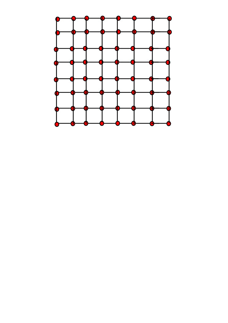
Figure 10: The dual graph of the partition $\mathcal{P}_{2}$.

Theorem 6.

For the two bi-affine IFS’s ${\mathcal{F}}=\{\mathchoice{\vbox{\vbox{\hrule height=0.8pt\hbox{\vrule width=0.8pt,height=6.0pt\kern 6.0pt\vrule width=0.8pt} \hrule height=0.8pt}}}{\vbox{\vbox{\hrule height=0.8pt\hbox{\vrule width=0.8pt,height=6.0pt\kern 6.0pt\vrule width=0.8pt} \hrule height=0.8pt}}}{\vbox{\vbox{\hrule height=0.3pt\hbox{\vrule width=0.3pt,height=2.1pt\kern 2.1pt\vrule width=0.3pt} \hrule height=0.3pt}}}{\vbox{\vbox{\hrule height=0.3pt\hbox{\vrule width=0.3pt,height=1.5pt\kern 1.5pt\vrule width=0.3pt} \hrule height=0.3pt}}}\,;\,f_{1},f_{2},f_{3},f_{4}\}$ and ${\mathcal{G}}=\{\mathchoice{\vbox{\vbox{\hrule height=0.8pt\hbox{\vrule width=0.8pt,height=6.0pt\kern 6.0pt\vrule width=0.8pt} \hrule height=0.8pt}}}{\vbox{\vbox{\hrule height=0.8pt\hbox{\vrule width=0.8pt,height=6.0pt\kern 6.0pt\vrule width=0.8pt} \hrule height=0.8pt}}}{\vbox{\vbox{\hrule height=0.3pt\hbox{\vrule width=0.3pt,height=2.1pt\kern 2.1pt\vrule width=0.3pt} \hrule height=0.3pt}}}{\vbox{\vbox{\hrule height=0.3pt\hbox{\vrule width=0.3pt,height=1.5pt\kern 1.5pt\vrule width=0.3pt} \hrule height=0.3pt}}}\,;\,g_{1},g_{2},g_{3},g_{4}\}$ defined above, the map $h=\pi_{G}\circ\tau_{F}$ is a homeomorphism.

Proof.

For each $n\geq 0$, let $\Omega_{n}$ denote the set of strings of length $n$ using symbols $\{1,2,3,4\}$ For the IFS $\mathcal{F}$, define a partition ${\mathcal{P}}_{F}^{n}=\{P_{\sigma}\,:\,\sigma\in\Omega_{n}\}$ of       recursively by taking ${\mathcal{P}}_{F}^{0}={\mathcal{P}}_{F}$ and

$${\mathcal{P}}_{F}^{n+1}=\{P_{\sigma\,j}=P_{\sigma}\cap f_{\sigma}(P_{j})\,:\,\sigma\in\Omega_{n},1\leq j\leq 4\}.$$

A straightforward induction shows that $\{M_{F}^{n}\}$ is a nested sequence of partitions of       . The dual graph $\Gamma_{F}^{n}$ of ${\mathcal{P}}_{F}^{n}$ is the grid graph shown in Figure 10 for $n=2$. This construction of a nested partition can be repeated for the IFS $\mathcal{G}$. Since the obvious graph isomorphisms between $\Gamma_{F}^{n}$ and $\Gamma_{G}^{n}$ are compatible with the nested partitions, Lemma 4 implies that $h$ is a homeomorphism. ∎

References

[1] R. Atkins, M. Barnsley, D. C. Wilson, A. Vince,
A characterization of point-fibred affine iterated function systems,
Topology Proceedings 38 (2010) 189-211.
[2] M. Barnsley, Transformations between self-referential sets, Amer. Math. Monthly 116 (2009) 291-304.
[3] M. Barnsley, Transformations between Fractals, Progress in Probability 61 (2009) 227-250.
[4] J. Hutchinson, Fractals and self-similarity, Indiana Univ. Math. J.30 (1981) 713-747.