Semi-blind Eigen-analyses of Recombination Histories Using CMB Data

Abstract

Cosmological parameter measurements from CMB experiments such as Planck, ACTpol, SPTpol and other high resolution follow-ons fundamentally rely on the accuracy of the assumed recombination model, or one with well prescribed uncertainties. Deviations from the standard recombination history might suggest new particle physics or modified atomic physics. Here we treat possible perturbative fluctuations in the free electron fraction, ${X_{\rm e}}(z)$, by a semi-blind expansion in densely-packed modes in redshift. From these we construct parameter eigenmodes, which we rank order so that the lowest modes provide the most power to probe the ${X_{\rm e}}(z)$ with CMB measurements. Since the eigenmodes are effectively weighed by the fiducial ${X_{\rm e}}$ history, they are localized around the differential visibility peak, allowing for an excellent probe of hydrogen recombination, but a weaker probe of the higher redshift helium recombination and the lower redshift highly neutral freeze-out tail. We use an information-based criterion to truncate the mode hierarchy, and show that with even a few modes the method goes a long way towards morphing a fiducial older Recfast $X_{\rm e,i}(z)$ into the new and improved CosmoRec and HyRec $X_{\rm e,f}(z)$ in the hydrogen recombination regime, though not well in the helium regime. Without such a correction, the derived cosmic parameters are biased. We discuss an iterative approach for updating the eigenmodes to further hone in on $X_{\rm e,f}(z)$ if large deviations are indeed found. We also introduce control parameters that downweight the attention on the visibility peak structure, e.g., focusing the eigenmode probes more strongly on the ${X_{\rm e}}(z)$ freeze-out tail, as would be appropriate when looking for the ${X_{\rm e}}$ signature of annihilating or decaying elementary particles.

1. Introduction

The Planck Surveyor is now well into its mission, observing the temperature and polarization anisotropies of the cosmic microwave background (CMB) with unprecedented accuracy (Planck HFI Core Team et al., 2011; Mennella et al., 2011). Both ACT (e.g., see Hajian et al., 2010; Dunkley et al., 2010; Das et al., 2011) and SPT (Lueker et al., 2010; Vanderlinde et al., 2010) are pushing the frontier of $TT$ CMB power spectra at small scales, and in the near future SPTpol (McMahon et al., 2009) and ACTPol (Niemack et al., 2010) will provide additional small scale $E$-mode polarization data, complementing the polarization power spectra obtained with Planck and further increasing the significance of $TT$ power spectra.

Using these datasets, cosmologists will be able to determine the key cosmological parameters with high precision (The Planck Collaboration, 2006; Tauber et al., 2010), making it possible to distinguish between various models of inflation (e.g. see Komatsu et al., 2011, for recent constraints from WMAP) by measuring the precise value of the spectral index of scalar perturbations, $n_{\rm s}$, and constraining its possible running, $n_{\rm run}$, as well as the tensor-to-scalar ratio, $r$. In addition many non-standard extensions of the minimal inflationary model are under discussion, and the observability of these possibilities with Planck(The Planck Collaboration, 2006) and future CMB experiment is being considered.

These encouraging observational prospects have motivated various independent groups (e.g. see Dubrovich & Grachev, 2005; Chluba & Sunyaev, 2006b; Kholupenko & Ivanchik, 2006; Switzer & Hirata, 2008; Wong & Scott, 2007; Rubiño-Martín et al., 2008; Karshenboim & Ivanov, 2008; Hirata, 2008; Chluba & Sunyaev, 2008; Jentschura, 2009; Labzowsky et al., 2009; Grin & Hirata, 2010; Ali-Haïmoud & Hirata, 2010) to assess how uncertainties in the theoretical treatment of the cosmological recombination process could affect the science return of Planck and future CMB experiments. The precise evolution of the free electron fraction, ${X_{\rm e}}$, with time influences the shape and position of the peak of the Thomson visibility function, which defines the last scattering surface (Sunyaev & Zeldovich, 1970; Peebles & Yu, 1970), and hence controls how photons and baryons decouple as electrons recombine to form neutral helium and hydrogen atoms. Consequently, the ionization history changes the acoustic oscillations in the photon-baryon fluid during recombination and therefore directly affects the CMB temperature and polarization power spectra. For the analysis of future CMB data this implies that in particular close to $z\sim 1100$ the ionization history better be understood at the $\sim 0.1\%$ level.

Probing the ionization history in time is equivalent to probing it in space with the light cone relating the two. Thus what we try to do in this paper, namely to come up with optimized probing functions for the recombination history, is quite akin to creating probes of the spatial structure of the boundary between HII and neutral hydrogen regions. Here of course we look from neutral to ionized, the cosmological recombination problem being an inside-out HII region, except in a predominantly electron scattering regime with a very large photon to baryon ratio which lowers the transition temperature between ionized and neutral.

The old recombination standard was set by Recfast (Seager et al., 1999, 2000), but its reliability for the precision cosmology was brought into question, e.g., by Seljak et al. (2003) . For the standard six parameter cosmology in particular our ability to measure the precise value of $n_{\rm s}$ and the baryon content of our Universe may be compromised if modifications to the recombination model of Recfast are neglected (Rubiño-Martín et al., 2010; Shaw & Chluba, 2011), introducing biases of a few $\sigma$ for Planck.

Currently it appears that all important corrections to the standard recombination scenario (SRS hereafter) have been identified (e.g., see Fendt et al., 2009; Rubiño-Martín et al., 2010, for an overview). The new recombination codes, CosmoRec (Chluba & Thomas, 2011) and HyRec (Ali-Haïmoud & Hirata, 2011) both account for these modifications to the SRS, superseding the physical model of Recfast and allowing fast and accurate computation of the ionization history on a model-by-model basis. CosmoRec and HyRec presently agree at a level of $\sim 0.1\%-0.2\%$ during hydrogen recombination, so that from standard recombination physics little room for big surprises seems to be left.

However, what if something non-standard happened? What if something was overlooked in the standard recombination scenario? From the scientific point of view the ionization history is a theoretical ingredient to the cosmological model, which usually is assumed to be precisely known and not subject to direct measurement. Clearly, it is important to estimate the possible level of uncertainty in the recombination model and to confront our understanding of the recombination problem with direct observational evidence. Here we describe how well future cosmological data alone are able to constrain possible deviations from the SRS.

In the past, several non-standard extensions of the recombination scenario have been considered. These include models of delayed recombination, in which hypothetical sources of extra photons that can lead to ionizations or excitations of atoms are introduced using simple parametrizations (Peebles et al., 2000). In particular, models of decaying (e.g., see Chen & Kamionkowski, 2004; Zhang et al., 2007) and annihilating particles (e.g., see Padmanabhan & Finkbeiner, 2005; Zhang et al., 2006; Hütsi et al., 2009; Slatyer et al., 2009; Hütsi et al., 2011) were discussed. In addition to extra photons, varying fundamental constants (e.g., see Kaplinghat et al., 1999; Scóccola et al., 2009; Galli et al., 2009) could affect the recombination dynamics in subtle ways.

All these ideas rely on a specific model for the (physical) process under consideration, with the derived constraints depending on the chosen parametrization. This minimizes the number of additional parameters, but does not allow us to answer questions about more general perturbations around the SRS and how well they can actually be constrained.

Here we approach this problem in a different way. We introduce perturbations to the SRS over a wide range of redshifts around hydrogen ($z\sim 1100$) and helium ($z\sim 1800$) recombination, using different basis functions. We then compute the corresponding signals in the CMB power spectra and perform a principle component decomposition to obtain eigenmode functions, ordered with respect to the level at which they can be constrained by the data. We study in detail how the eigenmodes depend on different experimental settings, the fiducial model, as well as the chosen parametrization for the recombination perturbations.

Our method is similar to the one used by Mortonson & Hu (2008), where the eigenmodes for different reionization scenarios ($6\lesssim z\lesssim 30$) were constructed. However, here we explicitly construct the mode functions at redshifts $z\gtrsim 200$, with particular attention to the dependence of the eigenmodes on different assumptions. We investigate how to use our prior knowledge of possible perturbations of the ionization history to choose the parametrization which is more preferred by the data. We also carry out a careful convergence study and show the equivalence of different basis functions (e.g., triangles, Gaussian bumps, Fourier series and Chebyshev polynomials). We particularly focus on the helium recombination problem, showing that in the absence of very tight constraints on the hydrogen recombination, we will not be able to unravel well remaining uncertainties in helium recombination with CMB data.

Similarly, small changes in the freeze-out tail of recombination are only weakly constrained, if possible ambiguities during hydrogen recombination are included.

Details of the general methodology to construct the eigenmodes for perturbations to ionization history are given in § 2. In § 3 we computed different eigenmodes over a rather wide redshift range ($z\in[200,3000]$). At the end of § 3, we develop a criterion which allows us to truncate the hierarchy of the eigenmodes based on their information content. In § 4 the modes are applied to two specific examples of ionization scenarios, illustrating how the method should be used with real CMB data. At the end of this section, we also discuss how the approach should be iterated if hints toward a considerable difference between the assumed and true model of recombination are indicated by the data. We close the paper by a brief discussion.

2. Methodology

In this section we introduce the approach and parametrization used to construct the principle components, or the eigenmodes, which will be used to describe possible corrections to the recombination scenario. Our method is mainly driven by the assumption of small relative perturbations around the fiducial model computed with the Recfast code (Seager et al. (1999); see Wong et al. (2008) for recent updates). As an example we have in mind the recombination corrections obtained with refined recombination models (Chluba & Thomas, 2011; Ali-Haïmoud & Hirata, 2011). However we also briefly discuss the possibility to constrain significant changes in the freeze-out tail of recombination and modes that mainly focus on helium recombination.

Throughout this paper the cosmic parameters, which will be referred to as the standard (cosmological) parameters, are $(\Omega_{\rm b}h^{2},\Omega_{\rm dm}h^{2},H_{0},\tau,n_{\rm s},A_{\rm s})$ as measured by WMAP7, unless stated otherwise. In several cases we also vary $Y_{\rm p}$ as a seventh parameter. Lensing is included in all simulations if not explicitly stated otherwise.

Figure 1.— The cosmological ionization history (left), ${X_{\rm e}}\equiv N_{\rm e}/[N_{\rm p}+N_{\rm HI}]$, and differential visibility function (right) for the standard recombination scenario with $T_{\rm CMB}=2.726$K (Fixsen, 2009) contrasted to a case with $T_{\rm CMB}=3$K. Here $N_{\rm p}$ and $N_{\rm HI}$ represent the number density of ionized and neutral hydrogen, while $N_{\rm e}$ denotes the number density of free electrons.

2.1. The standard recombination scenario

As explained in the introduction, the cosmological recombination history is one of the major theoretical inputs for computations of the CMB anisotropies. Consequently, high precision unbiased cosmic parameter measurements from current and future CMB experiments require a sufficiently accurate model for hydrogen and helium recombination.

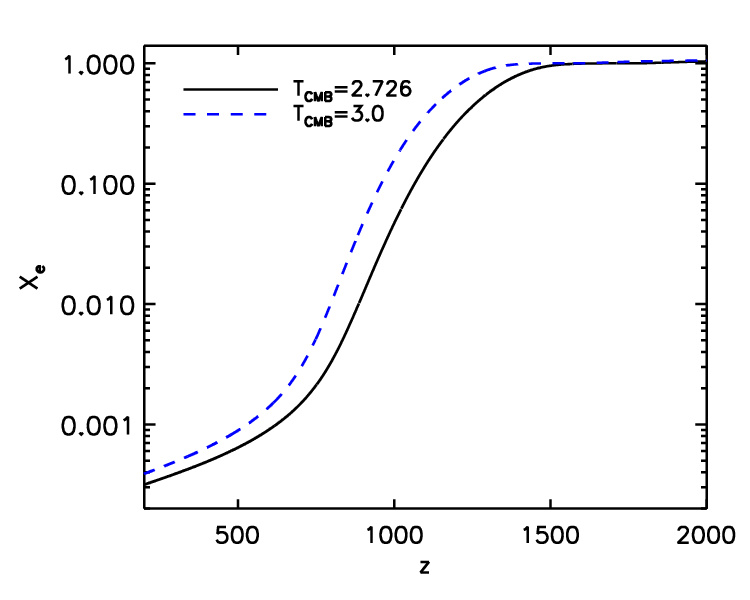
The ionization fraction for the SRS is shown in the left panel of Fig. 1. It was calculated using Recfast v1.4.2, which accounts for some of the modification to helium recombination (Kholupenko et al., 2007; Switzer & Hirata, 2008; Rubiño-Martín et al., 2008; Chluba & Sunyaev, 2010) using fudge parameters, but neglects detailed radiative transfer corrections (see Chluba & Thomas, 2011; Ali-Haïmoud & Hirata, 2011, and references therein) around $z\sim 1100$. The solid curve corresponds to an ionization fraction with the measured temperature of the CMB radiation, $T_{\rm CMB}\sim 2.726{\rm K}$ (Fixsen, 2009). For comparison and to illustrate the temperature dependence of the ionization history, the ionization fraction corresponding to $T_{\rm CMB}=3{\rm K}$ is also plotted (dashed curve). A larger value of $T_{\rm CMB}$ means more photons in the Wien tail of the CMB blackbody, so that the matter is kept ionized until lower redshift.

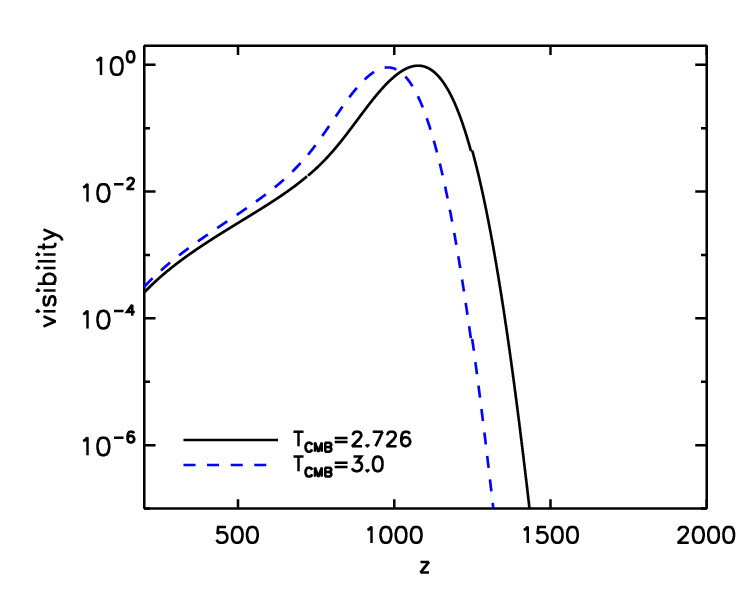
On the right the corresponding differential visibility functions (or visibility functions for short) are plotted:

$$g(z)\equiv-\frac{{\rm d}e^{-\tau(z)}}{{\rm d}\eta},$$ (1)

where $\eta$ is the conformal time and $\tau$ is the Thomson scattering optical depth from redshift $z$ to now.

The visibility function describes the probability that a photon we observe today last scattered off free electrons at a certain position along the line of sight. The CMB anisotropies formed mainly during the epoch of hydrogen recombination defined by the peak of the visibility function located at redshift $z\sim 1100$. They are thus most sensitive to changes around the maximum of visibility. For example, an increase in the width of the visibility bump corresponds to a more extended or slower recombination process, leading to more Thomson scatterings of photons off free electrons. These scatterings lead to the cancellation of the CMB anisotropies along the line of sight on scales comparable and smaller than the recombination width, while enhancing the polarization signal on larger scales. The location of the maximum of the visibility function for an assumed cosmological model, on the other hand, determines the distance to the last scattering surface. This in turn determines the positions of the peaks of the CMB power spectra. Similarly, any change in the ionization history, through affecting the visibility, would lead to (possibly measurable) changes in the CMB power spectra.

As the right panel of Fig. 1 indicates, at high redshifts $z\gtrsim 1400$ the visibility function falls off very quickly. At those times the number of free electrons is still so large that scatterings occur very frequently and the mean free path is very short. Consequently, the part of the ionization history which is connected to helium recombination mainly affects the damping tail of the CMB anisotropies, but even there the effect is rather moderate, as in the redshift range $1400\lesssim z\lesssim 3000$ helium can at most alter the number of electrons by $\sim 8\%$.

2.2. Choice of perturbation parametrization

We now introduce small perturbations to the SRS that allow construction of the eigenmodes.

There are different ways to parametrize the perturbations to the ionization history in a (semi-)model-independent way. For example, to study how well the low redshift ionization history ($z$ in the interval $[6,30]$) can be constrained by future CMB data, Hu & Holder (2003) and Mortonson & Hu (2008) used the changes in the ionization fraction in different redshift bins, $\delta{X_{\rm e}}(z)={\rm const}$, to parametrize the uncertainties. This is a valid choice for the low redshift region, because our ignorance of the underlying model of reionization does not suggest any preferred non-uniform weighting of the perturbations at different redshifts. In this regime $\delta{X_{\rm e}}(z)$ probes the ionization fraction itself and not perturbations guided by a fiducial model. The results from this choice of parametrization are shown to be fiducial model-independent which is expected due to the weak signal from the reionization process.

In contrast to this, at high redshifts ($z\sim 1100$) there is strong theoretical support for the exhaustively studied model of recombination in the realm of standard atomic physics and radiative processes. Also as it was mentioned in the introduction, the current generation of CMB data is sensitive to changes in ${X_{\rm e}}$ at the level of a few percent. Therefore the main assumption in this paper is that the fiducial model for the ionization history, ${X_{\rm e}^{\rm fid}}(z)$, is close to the true underlying history, ${X_{\rm e}}(z)$, which we are looking for. We call this method semi-blind emphasizing our belief in the SRS as the framework of recombination, with the search for deviations being limited to small perturbations around this reference model. The goal is to detect or place upper limits on these potential small deviations. Clearly, if data point toward significant deviations from the SRS, an iterative approach should be adopted, as will be discussed in § 4.4.

With small deviations in mind we can write:

$${X_{\rm e}}(z)={X_{\rm e}^{\rm fid}}(z)+\delta{X_{\rm e}}(z),$$

with $|\delta{X_{\rm e}}|/{X_{\rm e}^{\rm fid}}\ll 1$. A natural parameter to describe the perturbation is then the relative deviation in the ionization fraction:

$$\delta u(z)\equiv\delta{X_{\rm e}}(z)/{X_{\rm e}^{\rm fid}}(z)\quad\text{with}\quad|\delta u(z)|\ll 1.$$ (2)

This parametrization has the advantage of always satisfying the necessary condition ${X_{\rm e}}\geq 0$. It is also straightforward to fulfill the ${X_{\rm e}}\leq X_{\rm e,max}$ condition in the simulations, where $X_{\rm e,max}$ is determined by $Y_{\rm p}$, the primordial helium mass abundance, through $X_{\rm e,max}\simeq 1+Y_{\rm p}/2(1-Y_{\rm p})$. The parametrization in Eq. (2) weights possible perturbations at different redshifts by the fiducial ionization fraction. This implies that for $\delta u(z)=\rm const$ the absolute change in the ionization fraction $|\delta{X_{\rm e}}|$ is down-weighted in the freeze-out tail of ${X_{\rm e}}$ ($z\lesssim 800$; see Fig. 1), compared to perturbations around maximum visibility ($z\sim 1100$) where ${X_{\rm e}}\sim 1$. Throughout this paper $\delta u(z)$ as defined in Eq. (2) will be our main choice of parametrization.

A more general parameter which includes the above parametrization as a special case is given by:

$$\delta u(z)\equiv\delta{X_{\rm e}}(z)/[{X_{\rm e}^{\rm fid}}(z)+\sigma(z)],$$ (3)

where $\sigma(z)\geq 0$ can be a constant or otherwise convenient function of redshift allowing to focus on different redshift ranges of interest. In particular, when considering possible modifications to the ionization history introduced by energy injection, e.g. because of annihilating dark matter, or decaying relic particles (Chen & Kamionkowski, 2004; Padmanabhan & Finkbeiner, 2005; Zhang et al., 2006, 2007; Hütsi et al., 2009; Slatyer et al., 2009; Hütsi et al., 2011), where the freeze-out tail of recombination is disturbed, a value of $\sigma\gg{X_{\rm e}^{\rm fid}}$ would be a proper choice, giving higher weight to the perturbations in the lower redshift part (see § 3.4 and Fig. 10). In the limit of a high value of $\sigma$ relative to the fiducial ${X_{\rm e}}$ the parameters approach $\delta u(z)=\delta{X_{\rm e}}(z)$ which uniformly weights perturbations at different redshifts. This, as already discussed, is a good choice for regions where there is no strong a priori belief in the underlying model or if the redshifts of interest have comparatively low ${X_{\rm e}}$ where $\delta u(z)$ with $\sigma=0$ does not lead to strong enough signals to probe. In principle, a conveniently chosen redshift dependent $\sigma(z)$ is a tool to effectively incorporate our prior knowledge of the ionization history in the parametrization of its perturbations. For example, with $\delta u(z)$ defined by Eq. (3) one can smoothly interpolate between relative and absolute perturbations to ${X_{\rm e}}$, at high and low redshifts respectively. Also it is clear that one can focus on different parts of the recombination history by limiting the redshift range over which the eigenmodes are constructed [e.g., just on reionization ($0\lesssim z\lesssim 30$) or helium recombination ($1400\lesssim z\lesssim 3000$)].

2.2.1 Alternative parametrizations

Instead of directly perturbing the ionization fraction, as we chose here, it is plausible to parametrize possible changes in the physical sources of perturbation to the ionization history, such as energy injection in the medium which leads to excitation or ionization of atoms, or the ${\rm Ly}\alpha$ escape probability during recombination (see introduction). For example Mitra et al. (2010) chose the number of photons in the IGM per baryon in collapsed objects as the parameter to study the low redshift ionization history. Alternatively, one could modify the fudge factors or functions in Recfast, or alter the expansion rate given by the Hubble factor, $H(z)$.

Each of these possibilities implies different priors on the regions that can be altered and, e.g., in the case of $H(z)$ other aspects of the cosmological model are also affected. They also cover, in general, only a limited class of changes to the recombination history. When interested in perturbations to the ionization history, ${X_{\rm e}}$ is the physical quantity which, via the visibility function and the optical depth, most directly enters the Boltzmann equations which describe radiation anisotropies and can be solved using the Boltzmann codes such as Camb (Lewis et al., 2000) or Cmbfast (Seljak & Zaldarriaga, 1996). The ionization fraction has the additional advantage, over the visibility and the optical depth, of being straightforward to limit to physically allowed values. The nearly direct mathematical encounter of ${X_{\rm e}}$ with CMB anisotropies guarantees that any perturbation in the plasma that would lead to changes in the radiation anisotropies should go through and thus be reflected in ${X_{\rm e}}$. Therefore the relative changes in ${X_{\rm e}}$ constitute our preferred physical parameters.

We close by mentioning that, it is also theoretically possible to consider different variables for time such as (conformal) time, optical depth and scale factor. However, for our purpose we choose to work with redshift to describe temporal dependence. In principle different parametrizations, if they cover the same range of physical perturbations, can be transformed to one another with the proper change of the a priori distribution of parameters. Here, in the absence of physically motivated constraints, a uniform prior is assumed for perturbations at different redshifts regardless of parametrization (here, e.g., for various values of $\sigma$ in Eq. (3)). If the perturbation is strongly constrained by data, the choice of the prior would not play a major role.

Figure 2.— Perturbations in the ${X_{\rm e}}$ history, in the form of $M_{4}$ splines (left) and the derivatives of the $C_{\ell}$’s with respect to the amplitude of each perturbation ($TT$ power spectrum in the center, $EE$ on the right).

2.3. Basis functions and their different characteristics

Having chosen the parametrization, we now expand the perturbations in a discrete set of mode (or basis) functions, $\varphi_{i}(z)$:

$$\delta u(z)=\sum_{i=1}^{N}y_{i}\,\varphi_{i}(z)+r(z)~{}~{}~{}~{}~{}~{}z_{\rm min}\leq z\leq z_{\rm max}$$ (4)

and $\delta u(z)=0$ elsewhere. Here $r(z)$ is the residual and $y_{i}$’s are the parameters defining the strength on the mode $\varphi_{i}(z)$. Often we take $\varphi_{i}(z)$ to be localized in $z$ about a knot value $z_{i}$, but this is not necessary. We can, for example, choose the $\varphi_{i}(z)$ to form a complete orthonormal set in which case $N\rightarrow\infty$ and the residual $r$ would be zero. Below, we will discuss different possibilities for the choice of the mode functions.

2.3.1 Localized basis functions

We first investigated localized Gaussian and triangular bumps as mode functions. Both can be considered as approximations to the Dirac $\delta$-function. We define the $i$th basis function centered at redshift $z_{i}$ and having width $\sigma_{i}$ by:

$$\varphi_{i}(z)\propto\exp\left(-{\frac{[z-z_{i}]^{2}}{2\sigma_{i}^{2}}}\right)$$ (5)

for the Gaussian case and by

$$\varphi_{i}(z)\propto\left\{\begin{array}[]{ll}1-\frac{|z-z_{i}|}{\sigma_{i}}&\mbox{ $|z-z_{i}|<\sigma_{i}$},\\ 0&\mbox{otherwise},\end{array}\right.$$ (6)

for the triangles. Triangular bumps were used earlier in the principle component analysis of different reionization scenarios (Hu & Holder, 2003; Mortonson & Hu, 2008). In some circumstances, the sharp edges in the triangles could cause numerical problems. Smoothed localized functions such as Gaussians and the $M_{4}$ splines introduced below have numerical advantage.

As basis functions, it is more convenient if the set of $\varphi_{i}$’s is an orthogonal set. For this, there should be no overlap between different bumps. On the other hand, there is no way to cover the whole redshift range -a necessary condition for completeness- with a finite number of non-overlapping bumps. However, depending on the problem of interest, the width and separation of the (overlapping) bumps can be properly chosen to ensure all points in the redshift interval have been covered, while at the same time the orthogonality is not strongly violated.

Instead of Gaussian and triangular bumps, one can also adopt an approach similar to that used in Smoothed-Particle Hydrodynamics (SPH), and think of the basis functions as window functions (or kernels) used to interpolate the properties of particles to any point in the medium. For us, the particles would be the spline knots (e.g. see De Boor, 2001) at the specific $z_{i}$ with the associated magnitude $y_{i}$. There is a smoothing length $h$ associated with the kernel over which the properties of the particles are smoothed. A commonly used kernel (other than the Gaussian considered above) is the cubic $M_{4}$ spline (e.g. Monaghan, 2005), defined by:

$$\varphi_{i}(z) \propto M_{4}(|z-z_{i}|)$$

$$=\left\{\begin{array}[]{ll}\frac{1}{6}[(2-q)^{3}-4(1-q)^{3}]&\mbox{~{}~{}$0\leq q\leq 1$};\\ \frac{1}{6}(2-q)^{3}&\mbox{~{}~{} $1\leq q\leq 2$};\\ 0&\mbox{~{}~{} $q>2$ };\end{array}\right.$$ (10)

where $q=|z-z_{i}|/h$. Whereas the Gaussian kernel has non-zero contributions from every redshift (though the range is usually truncated beyond about $3\sigma$), the cubic spline is compact, reaching zero for particles beyond $2h$. (As discussed in § 3.2, we have used the smoothing length $h=1.5\delta z$ where $\delta z$ is the particle separation).

We modified the publicly available code Camb to simulate CMB power spectra for a more general recombination scenario that includes perturbations on top of the SRS. Introducing narrow features into the ionization history also required an increase in the redshift sampling of ${X_{\rm e}}$. We checked the numerical convergence and stability of the results by using high accuracy settings.

As examples for localized perturbations, Fig. 2 shows three perturbation functions $\delta u(z)=\delta\ln({X_{\rm e}})$ based on $M_{4}$ splines (left panel) and the corresponding $C_{\ell}$ response in $TT$ and $EE$. The perturbations are located at different redshifts and have equal widths. We see that the amplitude of the response typically increases at smaller scales indicating a change in the duration of the recombination epoch (i.e., the effective width of the visibility function). The $C_{\ell}$ response also has an oscillatory component similar to a change of the position of the visibility peak. These oscillations are most noticeable for the perturbations close to the visibility peak ($z\sim 1100$) and together with the overall slope of the $C_{\ell}$ response demonstrate that the perturbation effectively changes the duration as well as the redshift of the recombination.

Figure 3.— Similar to Fig. 2 but for perturbations in the form of Chebyshev polynomials.

2.3.2 Non-localized basis functions

In this part we expand the perturbations in terms of two non-localized basis functions which, unlike the localized case (with finite number of basis functions), do not suffer from non-orthogonality. If sufficiently many functions are taken into account, these basis functions, similar to the localized ones, can also be considered complete in practice.

The most commonly used set of non-localized basis functions is the Fourier series:

$$\varphi_{i}(z)\propto\cos(i\pi y)~{}~{}~{}~{}~{}~{}~{}i =0,1,2,...$$ (11a)

$$\varphi_{i}(z)\propto\sin(i\pi y)~{}~{}~{}~{}~{}~{}~{}i =1,2,...$$ (11b)

$$y=\frac{z-z_{\rm mid}}{\Delta z/2}$$ (11c)

where $\Delta z$ and $z_{\rm mid}$ are the width and central point in the redshift range of interest. Thus we have $|y|\leq 1$ as is required for Fourier expansion.

Alternatively, we can use Chebyshev polynomials of the first kind, $T_{i}$, to form the basis. These modes are constructed using the recursion formula:

$$T_{i+1}(x)=2x\,T_{i}(x)-T_{i-1}(x)$$

with initial conditions $T_{0}(x)=1$ and $T_{1}(x)=x$. In this case, the variable $x$ is replaced by $y$ as given by Eq. (11c). Chebyshev polynomials of the first kind are orthogonal with respect to the weight function $w(x)=1/\sqrt{1-x^{2}}$.

The non-local basis functions are very different in nature from the localized functions discussed in § 2.3.1. Therefore the response of the observables (here the $C_{\ell}$’s) to the perturbation $\delta u(z)$ in the form of these functions is also expected to be rather different. Figure 3 shows the $C_{\ell}$ responses when perturbing the ionization history using Chebyshev polynomials with different frequencies. We see that perturbations with low frequencies, covering a large redshift range, lead to $C_{\ell}$ responses with much larger mean amplitudes when compared to the perturbations in the form of local bumps (Fig. 2). However, as the frequency of the oscillations of the basis function increases, the response becomes weaker and its oscillations damp away. That is because neighbouring oscillations lead to similar responses in the $C_{\ell}$’s with opposite signs and can partially cancel out each other. In other words, the CMB power spectra are less sensitive to the very high frequency perturbations in the ionization history.

In principle, in the limit of large mode number, all bases work well. However, we have found that for the recombination history, although non-localized basis sets have their virtues, the $z$-localized bases are better, especially if we are trying to describe narrow features in redshift. We will return to this point in § 3.1.

2.4. Constructing the eigenmodes

We have so far introduced our choice of parametrization for characterizing potential perturbations to the ionization fraction and illustrated how the perturbations in the form of these parameters affect the CMB power spectra when expanded in different bases. In principle all the $q_{i}$’s (in Eq. (4)) are needed for a (nearly) complete reconstruction of a general perturbation $\delta u(z)$. However, in practice data cannot constrain the perturbations in detail in many cases. As we saw in Fig. 3, very high frequency perturbations are expected to lead to much smaller signals.

2.4.1 Eigenmodes with fixed standard parameters (XeMs)

To avoid dealing with many correlated (and possibly weakly constrained) parameters (i.e., the $q_{i}$’s), we construct a set of their linear combinations which are uncorrelated with each other and only keep those combinations that are most constrained by data. This procedure provides a hierarchy of mode functions and their corresponding signals in the CMB temperature and polarization power spectra. Exclusion of the weakly constrained eigenmodes does not affect the rest of the measurements since the eigenmodes describing the recombination perturbations are by construction uncorrelated.

If $N$ parameters are used to characterize the perturbations, i.e., $1\leq i\leq N$, the $N$ uncorrelated parameters will be determined by the eigenmodes of the ($N\times N$) Fisher information matrix:

$$F_{ij}\equiv-\left<\frac{\partial^{2}\ln p_{\rm f}}{\partial q_{i}\partial q_{j}}\right>,$$

where in the language of Bayesian analysis, $p_{\rm f}\equiv p({\bf q}|d,{\cal T})$ (with ${\bf q}=(q_{1},...,q_{N})$) describes the posterior probability of the parameters $q_{i}$’s for the given data $d$ in the theory space ${\cal T}$, i.e., an update from the prior probability distribution of the parameters, $p_{\rm i}=p({\bf q}|{\cal T})$ driven by the likelihood $p_{\rm f}={\cal L}({\bf q}|d,{\cal T})p_{\rm i}/{\cal E}$ where ${\cal L}({\bf q}|d,{\cal T})\equiv p(d|{\bf q},{\cal T})$ and the evidence ${\cal E}\equiv p(d|{\cal T})$ is a normalization factor. We include the ${\cal T}$ in the notation only if there is ambiguity in the theory space under consideration.

Under the assumption of uniform priors for the $q_{i}$’s, the Fisher matrix reduces to:

$$F_{ij}=-\left<\frac{\partial^{2}\ln{\cal L}}{\partial q_{i}\partial q_{j}}\right>.$$

The derivatives are calculated at the fiducial values of the parameters, in this case $q_{1}=...=q_{N}=0$. The ensemble average $\left<..\right>$ is over realizations of the CMB sky and instrument noise. In the standard CMB analysis with Gaussian signal and noise, we have ${\cal L}=\exp(-\Delta^{\dagger}{\bf C}^{-1}\Delta/2)/\sqrt{2\pi|{\bf C}|}$. Here $\Delta$ represents the temperature and polarization maps including both CMB signal and instrumental noise and ${\bf C}=\left<\Delta\Delta^{\dagger}\right>$ is the theoretical pixel-pixel covariance matrix. With this likelihood function, the Fisher matrix simplifies to:

$$F_{ij}=\frac{1}{2}{\rm Tr}\left({\bf C}^{-1}\frac{\partial{\bf C}}{\partial q_{i}}{\bf C}^{-1}\frac{\partial{\bf C}}{\partial q_{j}}\right).$$

In the limit of full sky observation, or in cut-sky cases where coupling between modes of different scales can be ignored, ${\bf F}$ can be written as:

$$F_{ij}=f_{\rm sky}\sum_{\ell=2}^{\ell_{\rm max}}\frac{2\ell+1}{2}\frac{\partial{\bf C}_{\ell}}{\partial q_{i}}{\bf C}_{\ell}^{-1}\frac{\partial{\bf C}_{\ell}}{\partial q_{j}}{\bf C}_{\ell}^{-1}$$ (12)

with

$$\bf{C_{\ell}}=\left({\begin{array}[]{cc}C_{\ell}^{T}e^{-\ell^{2}\sigma^{2}}+N_{\ell}^{T}&C_{\ell}^{TE}e^{-\ell^{2}\sigma^{2}}\\ C_{\ell}^{TE}e^{-\ell^{2}\sigma^{2}}&C_{\ell}^{E}e^{-\ell^{2}\sigma^{2}}+N_{\ell}^{E}\\ \end{array}}\right),$$

where we have included CMB temperature $T$, $E$-mode polarization and their cross correlation $TE$. Here $N_{\ell}^{T,E}$ stands for instrumental noise contribution to the power spectra and $\sigma$ is the width of the Gaussian beam. The effect of incomplete sky coverage has been naively taken into account by the $f_{\rm sky}$ multiplier which reduces the effective number of observed modes .

The Fisher matrix for $N$ parameters, as any other $N\times N$ real symmetric matrix, has $N$ independent eigenvectors which can be chosen to be orthogonal to each other and normalized to one. So ${\bf F}$ can be decomposed as ${\bf F}={\bf Sf}{\bf S}^{T}$ where the columns of ${\bf S}$ are the eigenvectors of ${\bf F}$ with their corresponding (non-negative) eigenvalues on the diagonal of the real diagonal matrix ${\bf f}$. The eigenmodes we are looking for can now be constructed using these eigenvectors of the Fisher matrix and the basis functions we started with:

$$E_{k}(z)=\sum_{i=1}^{N}S_{ik}\varphi_{i}(z).$$ (13)

If the $\varphi_{i}$’s happen to be orthonormal, then the eigenmodes $E_{k}(z)$ will be:

$$\int_{z_{\rm min}}^{z_{\rm max}}E_{k}(z)E_{k^{\prime}}(z)w(z){\rm d}z=\delta_{kk^{\prime}}.$$ (14)

Here $w(z)$ is the weight function with respect to which $\varphi_{i}$’s are orthonormal. Since Eq. (14) is not necessarily fulfilled, we enforce the $E_{k}(z)$’s to be normalized to unity (as a matter of convenience), which is equivalent to a renormalization of the eigenvectors of ${\bf F}$. Although in general this could change the rank ordering of the modes, in our case a reordering was not required. Now, instead of the original $\varphi_{i}$’s, the set of the eigenmodes can serve as basis functions for the expansion of perturbations (compare with Eq. (4)):

$$\delta u(z)=\sum_{k=1}^{N}\mu_{k}\,E_{k}(z).$$ (15)

To be more specific, we will refer to these parameter eigenmodes which describe perturbations to the ${X_{\rm e}}$ history by XeMs. In § 3.5 we will demonstrate two examples of perturbation reconstruction with different numbers of eigenmodes taken into account (Fig. 10). We will see how well these eigenmodes serve as basis functions and also which features of the original perturbations are restored (or lost) if only a subset of the eigenmodes are used in the reconstruction process.

The inverse square of the eigenvalues of the Fisher matrix can be used to forecast the error bars of the eigenmodes, i.e., $f_{ij}=\sigma^{-2}_{i}\delta_{ij}$, assuming the probability distribution of the parameters is multivariate Gaussian close to the maximum. For non-Gaussian likelihoods, the $\sigma_{i}$’s give the lower bound for the errors. In the rest of this paper we use the term error for the $\sigma_{i}$’s, as the Gaussianity of the likelihood function close to its maximum is usually a good assumption. If the modes are sorted in descending order of eigenvalues, the first few (with smallest $\sigma_{i}$’s) will be most constrainable. Thus, the constrainable part of the perturbations to the ionization history can be described by the eigenmodes which have reasonably small uncertainties (i.e., high eigenvalues), while the rest is practically unconstrainable by the dataset under consideration.

This procedure of using an orthogonal transformation to replace the parameters of the problem with a set of uncorrelated variables is called principal component analysis or PCA for short. (The parameter eigenmodes were used for CMB in Bond (1996) and subsequently in Bond et al. (1997) and many subsequent papers.) In general, the PCA needs to be applied to the whole history of ionization simultaneously (as well as the standard cosmic parameters), since we do not know a priori how the ambiguity in one epoch affects the measurements of the perturbations in other epochs. However, if it turned out that a particular period of ${X_{\rm e}}$ history could be relatively well constrained, e.g. by other probes, one could leave that epoch out of the perturbations. Moreover, choosing a suitable parametrization, potentially changing over time to properly take into account the different physics at different epochs, is a necessary but not straightforward task. In this work, the focus will be on the epoch of recombination since that is where the main CMB signal is coming from. A more complete analysis for the whole ionization history or where different parts of it are considered simultaneously is for future work.

Figure 4.— The six most constrained XeMs for five different basis functions (with 160 parameters). The maximum and width of the Thomson visibility function have been marked in all figures.

2.4.2 Eigenmodes with varying standard parameters

Above we assumed that the background cosmology was fixed and the parameter space only included perturbation parameters, i.e., $q_{i}$’s. However, as we will see in § 4.1, the eigenmodes constructed this way do not necessarily stay uncorrelated with one another when standard cosmological parameters are also being varied. Moreover, due to the correlation of the XeMs with one another as well as with the standard parameters, the constraints on the eigenmodes will possibly increase compared to the forecasted errors (reported in Table 1).

To avoid this issue, the eigenmodes of perturbations should be constructed in the presence of varying standard parameters. In this case the Fisher information matrix has the following general form

$$\bf{F} =\left({\begin{array}[]{cc}F_{ss}&F_{sp}\\ F_{ps}&F_{pp}\\ \end{array}}\right),$$ (18)

where we have ${\bf F}_{ss}=-\left<\frac{\partial^{2}\ln{\cal L}}{\partial s\partial s}\right>$, ${\bf F}_{sp}={\bf F}_{ps}-\left<\frac{\partial^{2}\ln{\cal L}}{\partial s\partial p}\right>$ and ${\bf F}_{pp}=-\left<\frac{\partial^{2}\ln{\cal L}}{\partial p\partial p}\right>$, with $s$ and $p$ symbolically representing the standard and perturbation parameters. To find the eigenmodes for perturbations after marginalization over the standard parameters, hereafter extended eigenmodes, or eXeMs, under the assumption of ellipsoidal parameter contours, we need to eigendecompose the perturbation block of inverse of the Fisher matrix, i.e., to find the eigenvectors of $({\bf F}^{-1})_{pp}$. However, the inversion of the Fisher matrix is numerically problematic as it is ill-conditioned due the non-constrainable parameters which exist in the parameter space under study.

In the case of fixed standard parameters, the Fisher matrix reduces to the perturbation block only, and since the eigenvectors of a symmetric matrix and its inverse are the same (with inverse eigenvalues), there is no need to invert the Fisher matrix before its eigendecomposition. Similarly to get the eXeM, i.e., the eigenvectors of $({\bf F}^{-1})_{pp}$ with ${\bf F}$ as in Eq. (18), we avoid the direct full inversion of ${\bf F}$ by noting that

$$({\bf F}^{-1})_{pp}=({\bf F}_{pp}-{\bf F}_{ps}{\bf F}_{ss}^{-1}{\bf F}_{sp})^{-1}.$$ (19)

The eigendecomposition of ${\bf F}_{pp}-{\bf F}_{ps}{\bf F}_{ss}^{-1}{\bf F}_{sp}$ then only requires the inversion of the well-behaved standard parameter block. It is straightforward to directly check that $({\bf F}^{-1})_{pp}$ properly describes the marginal likelihood of the perturbation parameters:

$${\cal L}({\bf p}|d)\propto e^{-{\bf p}^{T}{\bf F}_{pp}{\bf p}/2}\int e^{-{\bf s}^{T}{\bf F}_{ss}{\bf s}/2}e^{-{\bf p}^{T}{\bf F}_{ps}{\bf s}}{\rm d}{\bf s}$$

$$\propto e^{-{\bf p}^{T}({\bf F}_{pp}-{\bf F}_{ps}{\bf F}_{ss}^{-1}{\bf F}_{sp}){\bf p}/2}.$$

Here ${\bf p}$ and ${\bf s}$ are the arrays of the perturbation and standard parameters.

The eXeMs are then uncorrelated with each other (but not necessarily to the standard parameters) even in the presence of varying standard cosmic parameters. We will use this method later in § 3.8 to find the eXeMs describing the perturbations to recombination history. Hereafter, we use the term eigenmode with the very general meaning and reserve XeM only for the eigenmodes if they are constructed with fixed standard parameters.

It is also possible to treat the standard parameters depending on the way they affect the power spectra. Among the standard parameters, $Y_{\rm p}$ has this unique property of influencing $C_{\ell}$’s only through its impact on ${X_{\rm e}}$. In other words, if we find the ${X_{\rm e}}$ template in ${X_{\rm e}}$ parameter space corresponding to $Y_{\rm p}$, i.e., ${\rm d}{X_{\rm e}}/{\rm d}Y_{\rm p}$, small changes in $Y_{\rm p}$ can be mimicked by properly changing the amplitude of this template while $Y_{\rm p}$ is left unchanged. Note that changes in other standard parameters either directly lead to changes in the CMB with no influence on ${X_{\rm e}}$ (such as $n_{\rm s}$ and $A_{\rm s}$), or have both direct and indirect (i.e., through ${X_{\rm e}}$) impacts on the CMB (such as $\Omega_{\rm b}$). Therefore, when including a $Y_{\rm p}$-like parameter in the analysis, we can restrict our search for the perturbation eigenmodes to the part of ${X_{\rm e}}$ space which is uncorrelated to the ${X_{\rm e}}$ template corresponding to this parameter as described above. In this way if perturbations to ${X_{\rm e}}$ are initially described by $N$ parameters, we will in the end have the $Y_{\rm p}$-like parameter or its associated template as one parameter and $N-1$ eigenmodes which are uncorrelated to the $Y_{\rm p}$-like parameter. These $N-1$ eigenmodes together with the $Y_{\rm p}$-like parameter fully parametrize the original $N$-dimensional space of the perturbations. However, for the purpose of this work we did not further explore this possibility.

3. Perturbation eigenmodes for Recombination

In this section we follow the procedure explained in § 2.4 to find the eigenmodes for perturbations in the ionization fraction at high redshifts. For the most part we leave the standard parameters fixed, but return to the question of how these affect the mode functions later. We choose the redshift range of $[200,3000]$ which covers hydrogen and singly ionized helium recombination ($z\sim 1100$ and $z\sim 1800$ respectively) as well as part of the dark ages while being well above the standard reionization scenarios ($z\lesssim 30$). We assume the fiducial recombination history is given by the SRS, as explained in § 2.1, unless otherwise stated.

In the following we compare the eigenmodes generated by using various bases and study some of the aspects associated with them, such as their convergence and fiducial model dependence. Some consistency checks will also be presented. Special attention will be given to perturbation to helium recombination. We will also study how including the standard cosmic parameters in the analysis would change the eigenmodes of perturbations to the ionization history. At the end we propose an information-based criterion for cutting off the eigenmode hierarchy to be used in the data analysis.

Table 1The forecasted standard deviations of the first six XeMs from the Fisher analysis for different observational cases.

XeM	1	2	3	4	5	6
CVL($\ell_{\rm max}=3500$)	0.003	0.009	0.013	0.016	0.022	0.047
CVL($\ell_{\rm max}=2000$)	0.011	0.019	0.024	0.041	0.094	0.190
CVL($\ell_{\rm max}=3500$, T only)	0.004	0.021	0.064	0.103	0.208	0.275
Planck-ACTPol($\ell_{\rm max}=3500$)	0.015	0.047	0.068	0.13	0.22	0.31

3.1. XeM construction using different bases

In this section we take $\delta u(z)=\delta\ln{X_{\rm e}}$ and try the five different sets of basis functions described in § 2.3: Chebyshev polynomials and Fourier series as orthogonal non-local functions of redshift, and $M_{4}$ splines, triangular and Gaussian bumps as localized functions. For the latter three, the width of the bumps is chosen to be independent of redshift. We choose $\sigma_{i}=\delta z/2$ for Gaussian and triangular bumps (Eqs. (5) and (6)) and $h=1.5\delta z$ for $M_{4}$ splines (Eq. (10)). In all cases, $\delta z=\Delta z/(N+1)$ is the spacing between the centers of adjacent bumps, where $\Delta z$ is the redshift range of interest and $N$ is the number of basis functions used. For each set of basis functions we calculate the $N\times N$ Fisher information matrix as explained in § 2.4 where the $N$ parameters are the amplitudes of the perturbations in the form of the basis functions, i.e., $q_{i}$’s in Eq. (4). The standard cosmic parameters are fixed to their fiducial values. For the data we simulate the $T$, $E$ and $TE$ spectra up to $l=3500$ for a full-sky, cosmic variance-limited (hereafter CVL) CMB experiment, unless otherwise stated. We then construct the Fisher matrix (Eq. (12)) and from it the $N$ XeMs (Eq. (13)). The first six XeMs for $N=160$ are shown in Fig. 4. The first row in Table 1 shows the forecasted errors of these XeMs, obtained from the eigenvalues of the Fisher matrix. Note that including standard parameters in the analysis, e.g. MCMC simulations, can increase the error bars, as we will see later in § 4.

We can see that the first six XeMs – which are the most constrained modes – all have the strongest variations close to the maximum of the Thomson visibility function. The freeze-out tail is not perturbed significantly, and the oscillations around helium recombination ($z\sim 1800$) have much smaller amplitude than those at $z\sim 1100$. This is expected since the CMB anisotropies are most sensitive to perturbations during maximum visibility and features at low and high redshift are not weighing as much in the CMB power spectra, once uncertainties close to $z\sim 1100$ are allowed. This in turn implies that only once the ionization history during hydrogen recombination is known well can small modifications in the freeze-out tail or at $z\gtrsim 1400$ be constrained.

We can observe another aspect of the XeMs. The larger the expected error bar the more small scale structure or high frequency oscillations the modes have and the further away from the visibility peak they probe. This is again understandable, since neighbouring ups and downs in the mode functions lead to partial cancelation of the effect on the $C_{\ell}$’s. Once several oscillations are occurring close to $z\sim 1100$, signals produced farther away from maximum visibility can start competing with those from $z\sim 1100$, and hence become constrainable by the data.

We also see that the first few XeMs are practically the same independent of the chosen expansion basis (Fig. 4), although individual perturbations in different bases lead to totally different $C_{\ell}$ responses (Figs. 2 and 3). Moreover, these modes are converged and do not change by including higher modes, as we will see in § 3.2. However, as we go to modes with higher uncertainty (not shown here), the XeMs from different bases start to slightly differ from each other. A larger number of basis functions are required to make these higher XeMs agree as well. Moreover, we found that the higher (poorly constrained) XeMs, in particular from the extended basis expansions such as Fourier, become dominated by numerical noise. The reason is that for weakly constrained modes where the higher frequencies start to play a more important role, the impact of adjacent ups and downs from the high frequency perturbations (e.g. sine functions) may not be well resolvable in the $C_{\ell}$’s, resulting in their net effect being dominated by numerical noise. For the localized basis functions, as long as the individual bumps are numerically resolvable, we do not find this issue, because each perturbation has just one bump with no destructive neighbour.

For more precise computations of the higher XeMs improvements of the numerical treatment in Camb would become necessary. We tried several obvious modifications, as well as different settings for the accuracy level, but were unable to stabilize the results for very high frequency modes. However, since in the analysis we are hardly using more than a few XeMs, for the purpose of this work this was sufficient.

Figure 5.— Testing the convergence of the eigenmodes. Here, the six most constrained XeMs are shown for cases with different number of parameters (40, 80, 160 and 320) and with $M_{4}$ splines as the basis functions. We see that the modes for 160 and 320 parameters are basically the same, indicating that these modes have already converged with 160 parameters.

Figure 6.— The three most constrained XeMs for three different fiducial models. The default model corresponds to the SRS and the effect of gravitational lensing on the CMB anisotropies has been included. One model corresponds to a recombination history with a different CMB temperature and in the other model lensing is not included. For the case of the two different CMB temperatures, the major difference is the shift in the eigenmodes associated to the shift in the fiducial ${X_{\rm e}}$ and visibility functions (see Fig. 1).

3.2. Convergence test

In all cases considered above the number of modes was chosen to be $N=160$. We tested the convergence of the XeMs by trying $N=40$, $80$, $160$ and $320$ in different bases and found that by $N=160$ the first few modes are converged. Fig. 5 shows a representative example of this convergence with $M_{4}$ splines as the basis. Thus the few constrainable XeMs are independent of the very high frequency (or highly localized) perturbations and including basis functions of higher order will not affect these eigenmodes.

For the case of $M_{4}$ spline functions the robustness of the results should also be checked against increasing the width of the kernel. By comparing the (first six) XeMs with $h=1.5\delta z$ (as explained in § 3.1) to those with $h=3\delta z$, we conclude that the modes have already converged for $h=1.5\delta z$ and thus we will adopt $h=1.5\delta z$ in the rest of this paper.

3.3. Fiducial model and dataset dependence

It is important to note that the XeMs are by construction fiducial model dependent. In principle, the observables (such as $C_{\ell}$’s) for different fiducial models respond differently to the same perturbations depending on the strength of the signals, at different redshifts, from the unperturbed fiducial model.

As an example, in Fig. 6 we compare the eigenmodes for three fiducial ${X_{\rm e}}$ histories. Two of the models have different CMB temperatures and in the third one lensing has not been included. In the first two, the different $T_{\rm CMB}$’s lead to different fiducial ${X_{\rm e}}$’s. Here, the main difference in the eigenmodes is their shift towards lower $z$’s for the case with higher CMB temperature. This is consistent with the delayed recombination shown in Fig. 1, remembering that XeMs are primarily localized around the maximum of visibility where the $C_{\ell}$’s are most sensitive to. For the latter case with no lensing, although ${X_{\rm e}}$ and the physics around recombination have not changed, there are still slight changes in some of the XeMs as seen in Fig. 6.

We also checked the robustness of the eigenmodes against changes in the fiducial value of the parameters and the assumed reionization scenario. We tried a different value for $\Omega_{\rm b}$, as the parameter most strongly affecting the ionization fraction, $1\sigma$ away from its fiducial value. For the late reionization we tried an extended reionization scenario (i.e., ${X_{\rm e}}=1$ for $z\leq 6$; ${X_{\rm e}}=0.5$ for $6<z\leq 30$ and ${X_{\rm e}}=0$ elsewhere) radically different from our sharp fiducial reionization model (the default in Camb). For both of these tests the first six eigenmodes were found to be the same as our main eigenmodes (Fig 4) with tiny differences in the fifth and sixth modes for the latter case.

This implies that, although the eigenmodes are fiducial model dependent, the constrainable ones are not practically sensitive to changes in the fiducial model or its parameters in the limits currently allowed by the data for the standard model of cosmology. That is because small changes in the fiducial parameters and the corresponding small changes in the ionization history only affect the XeMs at second order. Here by small we mean changes that lead to (smaller than or) the same order of magnitude signal in the simulated data as the (few best) XeMs. The higher XeMs with larger uncertainties are more affected by the same changes in the fiducial parameters, as these changes are no longer considered small relative to these poorly constrained XeMs. This non-sensitivity of the best modes to the fiducial values of parameters does not contradict their significant correlation once the standard parameters are also allowed to vary, as we will see later in § 4.1.

Figure 7.— The three most constrained XeMs with and without polarization and with $\ell_{\rm max}=2000$ and $3500$.

Figure 8.— The three most constrained XeMs for a Planck-ACTPol-like experiment compared to a CVL experiment.

Figure 9.— The six most constrained XeMs with $\delta u(z)=\delta\ln(x+\sigma)$ as the parameter, having three different values for $\sigma$, and with Gaussian bumps as the basis functions.

Figure 10.— The reconstruction of two physically motivated ${X_{\rm e}}$ perturbation scenarios on (different number of) XeMs generated with Gaussian bumps (top) and the relative difference in the temperature power spectrum between the reconstructed perturbations and the full corrections (bottom). Right: The perturbations come from deviation from physical corrections to the recombination process (CT2010). Here the perturbation parameter is $\delta\ln({X_{\rm e}})$. Left: The perturbations are due to a model of dark matter annihilation. As the perturbation parameter we used $\delta\ln({X_{\rm e}}+0.01)$ to better accommodate for the freeze-out perturbation. A case with $\delta u(z)=\delta\ln({X_{\rm e}})$, i.e., $\sigma=0$, is shown for comparison.

We also studied the dependence of the XeMs on some properties of the simulated CMB datasets used for their construction, such as different $\ell_{\rm max}$ corresponding to the smallest scale information present in the data, and different experimental noise levels. The results for a CVL experiment up to $\ell=2000$ in temperature and polarization and also a CVL experiment only sensitive to temperature (up to $\ell=3500$) are shown in Fig. 7. As a more experimentally motivated case, we calculated the XeMs for simulated Planck-like data (using $100$, $143$ and $217$ GHz channels, with effective galaxy-cut sky coverage of $75\%$) and ACTPol-like data, including both wide and deep surveys (Niemack et al., 2010). As shown in Fig. 8, there is a tiny shift in the first mode relative to the mode for an ideal experiment and the changes grow as we proceed to higher modes.

More significant than the small changes in the XeMs constructed with different assumptions about data, are the forecasted error bars in different cases (see Table 1). By removing the temperature at high $\ell$’s or the polarization spectrum, the constraints on the amplitudes of the modes, determined from the eigenvalues of the Fisher matrix, become considerably larger. All these errors are calculated with the standard parameters fixed. However, the considered cases illustrate the general behaviour of the method. Taking into account the correlation between the perturbations and the standard cosmic parameters leads to relatively higher error bars, depending on the dataset used. We will return to this point later (table 3).

3.4. Alternative parametrizations for perturbations

We now turn to the parametrization defined by Eq. (3), $\delta u(z)=\delta\ln({X_{\rm e}}+\sigma)$ with $\sigma>0$. As mentioned earlier, this parametrization allows us to focus the perturbations on the freeze-out tail which are more difficult to recover with $\delta u(z)=\delta\ln({X_{\rm e}})$. This is because choosing $\sigma>0$ results in over-weighting the signal from the perturbations at low $z$ (with low ${X_{\rm e}}$) compared to a case with $\sigma=0$ for the same value of $\delta u(z)$.

Fig. 9 shows the six most constrained XeMs with $\delta u(z)=\delta\ln({X_{\rm e}}+\sigma)$ for different values of $\sigma$, all constructed by using 160 Gaussian bumps as the basis functions and assuming CVL experiment up to $\ell_{\rm max}=3500$. We see that the amplitude of the XeMs increases in the freeze-out tail as $\sigma$ increases. It will be illustrated in § 3.5 that a relatively high value for $\sigma$ is the preferred choice for studying perturbations that most significantly alter the freeze-out tail.

3.5. Consistency check: eigenmodes as a complete basis

Any function ${X_{\rm e}}(z)$ (in the redshift range under consideration) can be expanded in terms of these XeMs unless it has highly localized features compared to the highest frequency present in the basis functions or to the width of the bumps in the case of localized modes. That is because the XeMs are just linear combinations of the original basis functions, and thus cannot have frequencies higher than the maximum frequency present in the basis functions. On the other hand, as is clear from Fig. 4, strongly localized features in possible perturbations to recombination history are not constrained with CMB datasets. Therefore the lost features of an ionization model via expansion by these eigenmodes will not be measurable even if modes with higher frequencies are included in the analysis. In other words, the XeMs serve as a complete basis for the expansion of constrainable features in the possible perturbations in the recombination history.

To demonstrate the reconstruction of perturbations using the XeMs we choose two physically motivated ionization perturbations, one associated with physical corrections to the recombination process (Chluba & Thomas (2011), hereafter CT2010) and the other due to energy injection coming from a model of dark matter annihilation (using the description of Chluba, 2010).

3.5.1 Standard recombination corrections

The modification to ${X_{\rm e}}$ corresponding to CT2010 is shown in the top left panel of Fig. 10 (black solid line). This correction should be added to the ${X_{\rm e}}$ from the original version of Recfast (or the ${X_{\rm e}}$ from Recfast v1.4.2 setting ${\rm He_{Switch}}=0$). At high redshifts one can see the effect of accelerated helium recombination caused by absorption of photons in the Lyman continuum of hydrogen. During hydrogen recombination the corrections are caused by detailed radiative transfer effects as well as two-photon and Raman scattering events. The freeze-out tail is slightly higher than obtained with Recfast because of deviations from statistical equilibrium in the angular momentum sub-states. We note that with Recfast v1.5 a large part of all these corrections can be accounted for, however, these corrections are not explicitly modelled using a physical description but have been fudged to reproduce the results obtained with detailed recombination codes.

Table 2The projection of the modifications to recombination history on the first six XeMs.

XeM	1	2	3	4	5	6
CT2010	-0.32	0.08	0.16	0.02	-0.09	0.25
DM annihilation	-0.31	-0.30	0.46	-0.14	0.33	0.88

We project this $\delta\ln({X_{\rm e}})$ on the 160 XeMs constructed from perturbations in the recombination history in the form of Gaussian bumps and with the perturbation parameter being $\delta u(z)=\delta\ln({X_{\rm e}})$ for the CVL case with $\ell_{\rm max}=3500$, as described in § 3.1. The figure compares the reconstructed perturbation for three cases with different number of XeMs included. First note that by including all 160 XeMs the original perturbation is practically fully recovered. If only the 15 most constrained modes are included, the helium correction ($z\sim 1800$) and also hydrogen correction around $z\sim 1100$ are well restored while for lower $z$ regions higher modes are required. The reconstruction by six XeMs, however, is most sensitive to variations around $z\sim 1100$ and cannot tell much about the helium correction. The projection coefficients for the first six XeMs are shown in Table 2. For this particular model of corrections to the perturbation scenario we see that the XeM $1$, $3$ and $6$ are strongly dominant among the first six modes.

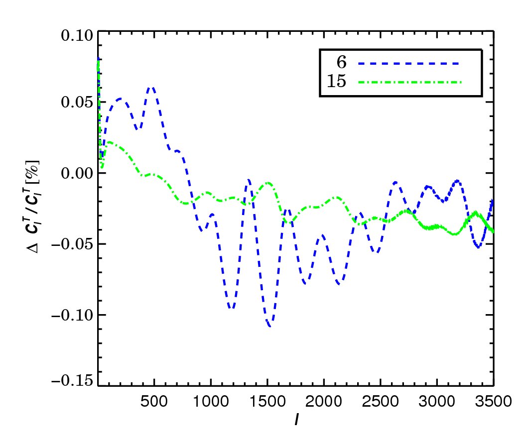
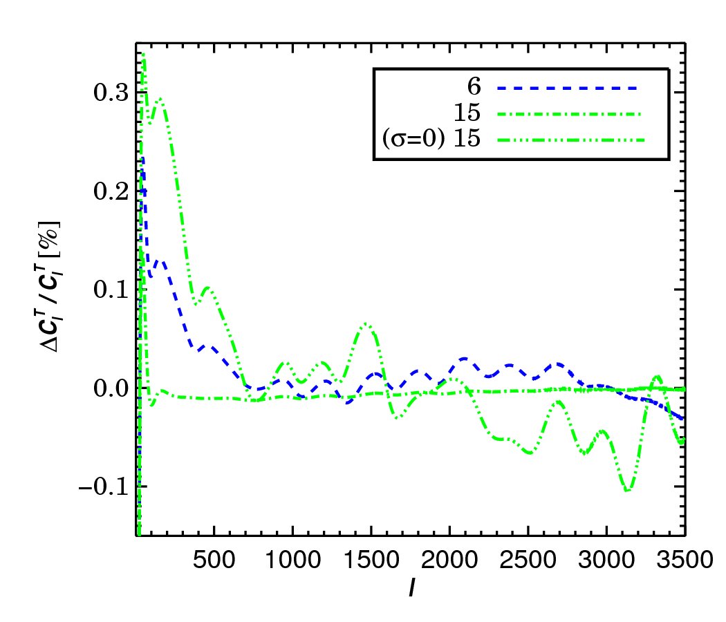
The lower left panel in Fig. 10 illustrates the relative difference between the temperature power spectrum for the reconstructed perturbations and the original full corrections. We see that with only six modes the error in the recovered $C_{\ell}$’s is less than $0.1\%$. Remembering that the changes in the $C_{\ell}$’s due to the full corrections are about a few percent, this shows that the main corrections to the CMB power spectra can be captured by just introducing a small number of modes. The CMB data indeed are not sensitive to all the details in the freeze-out tail of recombination and during helium recombination, unless prior knowledge renders uncertainties at $z\sim 1100$ very small. As we will see below, part of the corrections from higher modes are compensated for by biasing the XeMs included in the analysis.

Figure 11.— The $\delta{\rm vis}=({\rm vis}-{\rm vis}_{{\rm fid}})$ (left) and the relative changes in the $TT$ and $EE$ power spectra (middle and right) for the six most constrainable XeMs.

3.5.2 Dark matter annihilation scenario

As the second example we chose the perturbations arising from a model of dark matter annihilation. It was computed using the description of Chluba (2010) with an annihilation efficiency $f_{\rm DM}\sim 2\times 10^{-24}\,\rm eV/s$. The difference with respect to Recfast is shown in the right panel of Fig. 10. In contrast to the previous case, the perturbations here are not concentrated around the maximum of differential visibility but are most significant at lower redshifts. Therefore, for the decomposition of the DM perturbations we choose $\delta u(z)=\delta\ln({X_{\rm e}}+0.01)$ (see § 3.4 and Fig. 9) to allow a better recovery of the relatively large perturbations in the freeze-out tail without the need to include too many modes. This procedure can be interpreted as placing a strong prior on (physically) expected changes in the freeze-out tail.

The top right panel of Fig 10 shows the reconstructed perturbation including three different number of XeMs. Here the recovered curve becomes very close to the original perturbation by including the first 15 XeMs, while six XeMs have a poor recovery of the low-$z$ part. Note that the plots are illustrating $\delta\ln({X_{\rm e}}(z))$ although the XeMs and thus the decomposition of the perturbation are all performed with $\delta\ln({X_{\rm e}}+0.01)$.

For comparison the reconstruction of the perturbation with $\delta u(z)=\delta\ln({X_{\rm e}})$, i.e., with $\sigma=0$, and with 15 XeMs taken into account is also shown. As expected, this reconstruction is much poorer compared to the previous case with $\delta u(z)=\delta\ln({X_{\rm e}}+0.01)$ due to its lack of coverage of corrections in the freeze-out tail. This demonstrates that when there is prior knowledge in favour of the freeze-out tail of recombination being affected, a parametrization with $\sigma>0$ should be used in the analysis. However, it is still correct that the main signal is produced by the modifications close to $z\sim 1100$, even if the freeze-out tail apparently has the largest deviation from the SRS. This is why the first few mode functions for $\sigma=0$ do not have any strong low redshift tails. The eigenvectors naturally order the perturbations in the strength of the associated change in the CMB power spectra, as explained in § 3.1. This point is visible from the lower right panel where the $C_{\ell}$ difference is plotted for reconstructed perturbations with different number of modes included compared to the full perturbations. Similar to the previous case, these differences are several times smaller than the changes in the $C_{\ell}$’s caused by this model of DM annihilation, again meaning that these few modes can well capture the constrainable features of the perturbations.

Also if we look at the decomposition of the recombination correction into the first six XeMs (see Table 2) we see that they all have comparable contributions. This seems reasonable if we remember that the mode functions, despite being weighted toward the low redshift part, still have a significant component at high redshift which need to be cancelled out to recover this pattern of perturbation with its low redshift modification. Therefore the neighbouring modes have the same order of magnitude amplitude to properly cancel out the high redshift perturbations. This difference in the amplitude of the modes in principle allows us to distinguish this type of perturbation from those of CT2010.

3.6. Impact of the eigenmodes on differential visibility and CMB power spectra

It is worthwhile to see how the XeMs affect the visibility function and the CMB power spectra. The left panel in Fig. 11 shows the change in the visibility function (normalized to the maximum of the fiducial visibility) for the first six XeMs. It is remarkable that relative changes in ${X_{\rm e}}$ of a few percent close to the maximum of visibility, which lead to measurable effects in the CMB power spectra, only cause relative changes in the visibility of the order of $10^{-4}$. This confirms the high sensitivity of the $C_{\ell}$’s to tiny changes in the visibility.

From Fig. 11 we also see that the most constrained mode, XeM $1$, has an effect on the CMB power spectra consistent with changes the width of the visibility function and a slight shift of its peak position. The second mode corresponds primarily to a shift in the visibility peak. The higher XeMs, with their several peaks and valleys, lead to less trivial changes in the width and position of the visibility function.

Figure 12.— The six most constrained eXeMs. The solid blue lines correspond to modes constructed after marginalization over six standard parameters while for the dashed red curves $Y_{\rm p}$ is marginalized over in addition.

The relative changes in the CMB temperature and $E$-mode polarization power spectra due to the first six XeMs are illustrated in the middle and right panels of Fig. 11. To aid visual comparison, the amplitudes of the XeMs have been chosen equal to their associated $1\sigma$’s so that they would lead to comparable changes in the $C_{\ell}$’s. It is interesting to note that for XeM $1$, due to its narrower visibility width compared to the fiducial model, the high $\ell$ damping in the temperature and polarization anisotropies is smaller. At the same time, because of fewer scattering opportunities for the photons, this mode leads to less polarization (negative $\delta C_{\ell}^{E}$ at low $\ell$’s). The $C_{\ell}$ signal associated with the second mode has the strongest oscillatory behaviour, consistent with a shift in the position of the visibility function. The mainly oscillatory impact of XeM $4$ and $5$ on the $C_{\ell}$’s also suggests that an effective shift in the position of the visibility function is present, while for mode XeM $3$ and $6$ the tail of the power spectrum is strongly damped (thus the negative $\delta C_{\ell}^{T,E}$ at small scales), again corresponding to a change in the effective width of the visibility.

3.7. Perturbations to helium recombination

As mentioned early in this section, the redshift range chosen in our analysis of perturbations to ionization fraction includes the recombination of singly ionized helium. Some of the most constrained XeMs we found also extend up to $z\sim 1600$. These, therefore imply some impact from the helium recombination epoch on the XeMs.

One way to confirm this statement is to limit the redshift range of perturbations to mainly include singly ionized helium recombination, e.g., $[1500,3000]$, while the total ${X_{\rm e}}$ (from both hydrogen and helium) is perturbed. We observe that the XeMs constructed this way have comparably large values at the lower redshift boundary ($z=1500$) and would steeply go to zero if enforced by the imposed boundary conditions. This indicates that despite being restricted to the helium recombination epoch, the XeMs are still most sensitive to changes in the signal from the hydrogen recombination and changes in ${X_{\rm e}}$ due to the helium recombination are hardly constrainable, unless a properly chosen non-uniform prior on $\delta{X_{\rm e}}$ is imposed.

As already emphasized, the parameters $\delta u(z)$ only characterize relative changes in ${X_{\rm e}}$ and the full description of the ionization fraction depends also on the standard cosmic parameters as well as the relevant theoretical assumptions about the physics of recombination. Among the standard parameters, $Y_{\rm p}$ has a distinct role in describing an aspect of the ionization fraction complementary to $\delta u(z)$ by determining the maximum total number of electrons available at each redshift: $N_{\rm e,max}=N_{\rm e,max}^{\rm H}+N_{\rm e,max}^{\rm He}\approx(1-Y_{\rm p}/2)N_{\rm b}$, where $N_{\rm b}$ is the baryon number density. Therefore, although $Y_{\rm p}$, in the first instance, requires to be marginalized over when constructing the eXeMs due to its intimate relation with the ionization fraction, it is also legitimate to treat recombination perturbations and the maximum number of electrons available at each redshift separately.

In § 4.1 we will use MCMC to measure constraints on $Y_{\rm p}$ alongside the six standard parameters and the first few XeMs using (simulated) CMB data. Also in the next section, we explore how the eigenmodes change if they are marginalized over $Y_{\rm p}$.

Figure 13.— The first three eXeMs with only $Y_{\rm p}$ being marginalized over (dashed blue curves). For comparison, the first three XeMs are also plotted (solid black curves).

Table 3The forecasted standard deviations of the first six eXeMs from the Fisher analysis constructed by marginalization over different number of standard cosmic parameters and for different observational cases. In all cases, $\ell_{\rm max}=3500$.

eXeM	1	2	3	4	5	6
CVL, marg: six std	0.011	0.012	0.029	0.052	0.059	0.064
CVL, marg: six std + $Y_{\rm p}$	0.011	0.027	0.029	0.052	0.059	0.071
Planck-ACTPol, marg: six std	0.058	0.074	0.189	0.308	0.439	0.532
CVL, marg: $n_{\rm s}$, $A_{\rm s}$	0.009	0.011	0.016	0.018	0.033	0.059

3.8. eXeM construction

The XeMs we discussed so far were constructed with non-varying standard parameters and therefore can be considered as the limiting case of zero errors on the standard parameters. However, as mentioned earlier in § 2.4.2, the eigenmodes become correlated when they are simultaneously being measured with the standard parameters, due to their degeneracy with the standard parameters. The strength of the impact of these correlations on the XeM estimation depends on the (prior) constraints on the standard parameters. It is therefore worthwhile to see how the modes and their rank ordering change if the standard parameters are allowed to vary as well.

Figure 12 illustrates the first six eXeMs constructed after marginalization over the main six and seven (including $Y_{\rm p}$) standard parameters, constructed as described in § 2.4.2. The eXeMs have stronger high redshift features compared to the XeMs. This implies that the degeneracy between the standard parameters and some features in the perturbations of the ionization fraction has pushed back some patterns of high significance to lower levels opening up the room for some high redshift or higher frequency patterns which only had the chance to show up at lower significance XeMs.

The modes in the shown two cases (i.e., marginalized over six and seven standard parameters) differ only slightly. That is because $Y_{\rm p}$ is rather weakly constrained using CMB data alone and in the presence of other standard parameters its role in shaping the eigenmodes is only secondary. If, on the other hand, we hold the six standard parameters fixed and only let $Y_{\rm p}$ vary, the eigenmodes will be more significantly affected (see Fig 13). The reason is that $Y_{\rm p}$ is comparable in significance to small changes in the ionization fraction and marginalizing over it, without the dominance of the standard parameters, would lead to marked changes in the eigenmodes. The forecasted errors on the first six eXeMs with and without $Y_{\rm p}$ included is compared in Table 3. We see that the errors are mostly the same, again implying the subdominant role of $Y_{\rm p}$. In terms of the errors the most affected modes are eXeM 2 and 6.

Table 4The coefficients of projection of the six most constrained eXeMs on the first eight XeMs.

	XeM 1	XeM 2	XeM 3	XeM 4	XeM 5	XeM 6	XeM 7	XeM 8
eXeM 1	-0.00	-0.90	0.21	-0.29	-0.12	0.02	0.02	0.01
eXeM 2	-0.76	-0.05	-0.48	-0.35	0.16	-0.02	-0.02	-0.01
eXeM 3	-0.31	0.34	0.42	-0.38	-0.54	-0.41	0.02	-0.11
eXeM 4	-0.35	0.13	-0.48	-0.31	-0.50	0.27	-0.28	0.37
eXeM 5	0.24	-0.01	-0.15	-0.20	0.06	-0.48	0.63	0.49
eXeM 6	-0.19	-0.22	-0.07	0.41	0.00	-0.41	-0.55	0.49

Figure 14.— The best three eXeMs with the two inflationary parameters $A_{\rm s}$ and $n_{\rm s}$ being marginalized over, compared to the XeMs, where all standard cosmic parameters are held fixed in the construction process of perturbation eigenmodes.

3.8.1 Projecting eXeMs onto XeMs

It is instructive to see how the eXeMs can be constructed from the XeMs. Table 4 shows the coefficients of the projection of the first six eXeMs (Fig. 12) on the best eight XeMs (Fig. 4). Note that the most constrained eXeMs have their strongest projections along these first few XeMs and the contribution from all other modes is at most about a percent for these first six eXeMs. This means that allowing the standard parameters to vary mixes and rearranges the first few XeMs with negligible leakage from higher neglected XeMs.

More specifically, the first eXeM is very similar to XeM 2, with some contribution from XeM 3 and XeM 4. The second eXeM is mainly a combination of the first, third and fourth XeMs, and eXeM 3 and eXeM 4 have comparable contributions from the first six and eight XeMs, respectively. The eXeM 5 and 6 are dominated by higher modes (XeM 6-8). As a result the space covered by the first few XeMs is not practically hugely different from the space covered by the first few eXeMs if proper number of modes (here eight XeMs for six eXeMs) are included in the analysis. This implies that using similar number of XeMs and eXeMs in an analysis of possible recombination perturbations should give similar results for the reconstructed modification in the ionization history, at least for the CVL case where relatively large number of eigenmodes are included. The main advantage of the eXeMs is that one can obtain more realistic estimates for the error bars directly after the construction of these modes. Also the eigenmode measurement is robust against including new eigenmodes in the analysis if the eXeMs are used as the modes. However, it also turns out that the eXeMs perform better than the XeMs in the simulated analysis of Planck data, where only 1-3 modes seem to be constrainable.

3.9. From eXeMs to XeMs

The two sets of ionization perturbation eigenmodes introduced and constructed so far, i.e., the XeMs and the eXeMs, allow us to best describe and measure the uncertainties in the ionization fraction in the two extreme ends of our knowledge of the standard cosmic parameters. The eXeMs present a case where the tightest constraints on the standard (six) parameters are from CMB data alone. Therefore a simultaneous measurement of the standard parameters and the uncertainties in the ionization fraction, using the CMB dataset at hand, is required. The construction of the XeMs, on the other hand, assumes the standard cosmic parameters are measured with high accuracy from other cosmological probes and the CMB data are only used for the direct measurement of the ionization history. In other words, the XeMs, by ignoring the uncertainties in the standard parameters, extract the maximal amount of information that the CMB data would ever have to offer about the ionization fraction.

Between these two limiting cases, there is a gray region where, depending on the dataset at hand, tight priors from non-CMB surveys can be imposed on some of the standard parameters while the rest are marginalized over when constructing the eigenmodes. For example, if all standard parameters, but the inflationary ones $A_{\rm s}$ and $n_{\rm s}$, are measured to very high precision by other probes, such as large scale structure, baryonic oscillation, lensing and supernova surveys (e.g. LSST, Pan-STARRS, BigBOSS, WFIRST, EUCLID), the corresponding eigenmodes would be constructed after marginalization only over these inflationary parameters.

Fig 14 compares the first three XeMs with eigenmodes marginalized over $A_{\rm s}$ and $n_{\rm s}$. The forecasted errors on these eigenmodes (from the Fisher analysis) are presented in the last row of Table 3. Not surprisingly, these modes have smaller errors compared to the eXeMs which have been made after marginalization over six standard parameters, and have larger errors compared to XeMs (with no standard parameter varying). These modes and similar ones after marginalization over different sets of standard parameters smoothly bridge the gap between the XeMs and the eXeMs. Depending on the datasets available at the time of real data analysis, the proper eigenmodes marginalized over the appropriate standard parameters must be constructed. With the current (and very near future) surveys, the most realistic choice are the eXeMs, constructed according to the experiment under consideration, which should be quite similar to the Planck-ACTPol-like case studied here.

3.10. Criteria for truncating the eigenmode hierarchy

For the full reconstruction of perturbations to the ionization fraction, all eigenmodes are needed in principle since they form a complete basis set. In practice, sequentially adding modes rank ordered in the (possibly renormalized) eigenvalues $f_{k}=\sigma_{k}^{-2}$ of ${\bf F}$ from high to low gives a rapidly diminishing return once one goes beyond a dozen or so. And often we can learn much from using just the first few. As more modes are added, the width covered by the allowed ${X_{\rm e}}$ trajectories increases, as Figs. 22 to 26 in § 4.3 show. The errors in those standard cosmic parameters which are correlated with the ${X_{\rm e}}$ eigen-parameters also increase. On both counts, it behooves us to develop criteria for selecting which modes to keep, bearing in mind Occam’s Razor for minimizing the number of new parameters to be added. Thus we show in § 4 what happens when one mode, a few modes and a handful of modes are added. To be more quantitative, we explore a criterion based on not allowing the Shannon entropy to increase too much as the next eigenmodes in the hierarchy are added.

The information action is defined in terms of the a posteriori probability of the variables $p_{\rm f}$ and the evidence ${\cal E}$ as ${\cal S}_{\rm I,f}({\bf q})\equiv\ln p_{\rm f}^{-1}-\ln{\cal E}$. Recalling from § 2.4.1, the a posteriori probability $p_{\rm f}\equiv p({\bf q}|d,{\cal T})$ of variables ${\bf q}=(q_{1},...,q_{N})$ given the theory space ${\cal T}$ and the datasets $d$ is related to the a priori probability $p_{\rm i}\equiv p({\bf q}|{\cal T})$, the likelihood ${\cal L}({\bf q}|d,{\cal T})\equiv p(d|{\bf q},{\cal T})$ and the evidence ${\cal E}\equiv p(d|{\cal T})$ through Bayes theorem: $p_{\rm f}={\cal L}({\bf q}|d,{\cal T})p_{\rm i}/{\cal E}$. The information action can then be written in terms of $p_{\rm i}$ and ${\cal L}$:

$${\cal S}_{\rm I,f}({\bf q})=\ln p_{\rm i}^{-1}+\ln{\cal L}^{-1}\,.$$ (20)

For basic information theoretic and Bayesian notions and notations see, e.g., the MacKay (2003) textbook. The framework given here was used in a CMB context by Farhang et al. (2011).) For us the $q_{k}$’s are the amplitudes of the ordered eigenmodes for XeMs or eXeMs. Generally the fluctuations in the standard cosmic parameters from their maximum likelihood values are included along with these eigen-parameters. We shall assume the prior distribution of the parameters to be uniform in the $q_{k}$. The expansion of $S_{\rm I,f}$ to quadratic order is the basic perturbative approach used throughout this paper, leading to a Gaussian $p_{\rm f}$: ${\cal S}_{\rm I,f}({\bf q})\approx{\cal S}_{\rm I,m}+{\bf q}^{\dagger}{\bf F}{\bf q}/2$ in terms of the Fisher matrix and the information action minimum ${\cal S}_{\rm I,m}=-\ln(p_{\rm i}{\cal L}_{\rm max})$.

The posterior Shannon entropy is related to the final-state ensemble-average of the information action and the evidence:

$$S_{\rm f}\equiv{\langle\ln p_{\rm f}^{-1}\rangle}_{\rm f}={\langle{\cal S}_{\rm I,f}({\bf q})\rangle}_{\rm f}+\ln{\cal E}\,.$$

For the quadratic order expansion it is

$$S_{\rm f} \approx\frac{1}{2}\rm{Tr}\ln{\bf F}^{-1}+\frac{N}{2}\ln(2\pi)+\frac{1}{2}\rm{Tr}\left({\langle{\bf q}{\bf q}^{\dagger}\rangle}{\bf F}\right)$$

$$=\frac{1}{2}\rm{Tr}\ln{\bf F}^{-1}+\frac{N}{2}(\ln(2\pi)+1).$$

The second line follows from the first since the correlation matrix of the ${\bf q}$ is ${\langle{\bf q}{\bf q}^{\dagger}\rangle}={\bf F}^{-1}$. The associated evidence involves the information action minimum, $\ln{\cal E}\approx S_{\rm f}-{\cal S}_{\rm I,m}-\frac{N}{2}$.

The entropy associated with mode $n$ is

$$S_{n}\equiv-\frac{1}{2}\ln f_{n}+(1+\ln 2\pi)/2=S(\leq n)-S(\leq n-1)\,.$$

It is a finite difference of the total entropy of the first $n$ modes in the eigen-hierarchy,

$$S(\leq n)=\frac{n}{2}(1+\ln 2\pi)-\frac{1}{2}\sum_{k=1}^{n}\ln f_{k}\,$$

and

$${\langle s\rangle}_{n}\equiv S(\leq n)/n\,$$

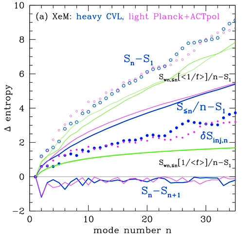
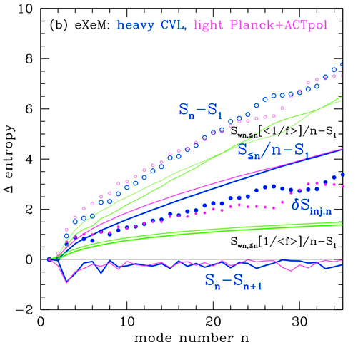
is the associated mean entropy-per-mode. Fig. 15 shows how the relative entropy $S_{n}-S_{1}$ and the mean entropy ${\langle s\rangle}_{n}-S_{1}=S(\leq n)/n-S_{1}$ grow with $n$ for the modes derived from the localized Gaussian expansion. We also plot two versions of ”white-noise” entropy.

$$S({\rm wn},\leq n)(\sigma^{2})\equiv n(\ln\sigma+(1+\ln 2\pi)/2),$$

$${\rm mean-variance}\ \sigma^{2}=\sum_{k\leq n}f_{k}^{-2}/n,$$

$${\rm mean-weight}\ \sigma^{2}=[\sum_{k\leq n}f_{k}^{2}/n]^{-1}.$$

These are entropies maximized subject to the constraint that we only have knowledge of the integrated $\sigma^{2}$, whereas $S(\leq n)$ is the maximized entropy given knowledge of the full spectrum $\{f_{k}^{-1}\}$. The mean-variance white noise lies above $S(\leq n)$ and the mean-weight white noise lies below. The mean-weight behaviour is dominated by a $\ln(n)$ rise, since the total weight of modes below $n$, $\ln\sum_{k\leq n}f_{k}^{2}$, quickly approaches a constant, reflecting the dominance of the high-weight eigenmodes in the sum.

We first discuss why we do not use the traditional evidence ratio often used in Bayesian theory to decide if a new parameter $q_{n}$ should be added. The log-evidence difference for the addition of $q_{n}$ is

$$\Delta\ln{\cal E}_{n} \equiv\ln{\cal E}(\leq n)-\ln{\cal E}(\leq n-1)$$

$$=S_{n}-1/2-\Delta{\cal S}_{\rm I,m}.$$

This requires evaluation of the change in the information minimum. It also has the usual disadvantage of depending upon the $f_{k}$ measure. Although using eigen-parameters ensures the same dimensionality for the different $f_{k}$, it does not fully remove this re-parameterization ambiguity since there can be a $k$-dependent scaling. (In fact, we have usually renormalized our $f_{k}$ so that the associated eigenmodes $E_{k}(z)$ have unit norm upon $z$-integration.)

Our preferred approach for hierarchy truncation is to use suitably-defined entropy differences. In particular we wish to set a threshold control on the injection entropy,

$$\delta S_{{\rm inj},n}=S_{n}-{\langle s\rangle}_{n}\,,$$

the entropy from adding mode $n$ relative to the mean-entropy from all $\leq n$ modes. It is related to the relative increase in phase space volume $V(\leq n)=\exp(S(\leq n)-n/2)=\exp(n({\langle s\rangle}_{n}-1/2))$ associated with mode additions:

$$\ln\left[V(\leq n+1)/V(\leq n)^{(n+1)/n}\right] =S_{n+1}-{\langle s\rangle}_{n}$$

We chose $S_{{\rm inj},n}$ instead because it is zeroed out for mode one, but $S_{{\rm inj},n}$ quickly approaches $S_{n+1}-{\langle s\rangle}_{n}$. For example, if we impose a $\Delta S_{\rm t}\sim 1/2$ threshold in Fig. 15 on the CVL XeM case, we would use only one mode, whereas $\Delta S_{\rm t}\sim 1$ picks up about 5, $\sim 3/2$ harvests about 10, and 2 gives about a dozen. Similar tales can be told for the eXeM CVL case and for both Planck+ACTpol forecasts.

Another more erratic measure is relative injection jumps, which is nearly $S_{n+1}-S_{n}$. In Fig. 15, the negative of this is plotted for clarity of presentation. Either reading off from the figure, or the using the lists of errors in Tables 1 and 3, the sample threshold $\Delta S_{\rm t}=1/2$ again yields only a mode or two.

The fluctuating nature of $S_{n+1}-S_{n}$ implies we can use it to split the modes into groups of similar information content which arise by thresholding it. If a mode is selected to be included in the analysis by, say, sharp-thresholding the injection entropy, it is logical that all of its co-modes be included, which is akin to softening the threshold. The groupings found with $\Delta S_{\rm t}=1/2$ imposed upon $S_{n+1}-S_{n}$ creates boundaries at one mode, five modes, and so on. These are, not surprisingly, similar to mode numbers obtained as we move the threshold on injection up, hence that criterion can be used instead to define mode groups.

Figure 15.— Various measures of entropy differences defined in the text are plotted against increasing eigenmode number, for (a) the XeM case and (b) the eXeM case. The Cosmic Variance Limited mode results have heavy lines or points, the Planck+ACTpol forecast has lighter lines and points, as indicated. They look quite similar. For this figure, the modes are determined by the densely-packed Gaussian bump expansion, but the triangular and spline expansions look similar, differences becoming notable only at higher $n$. The basic information on growing entropy is given by $S_{n}-S_{1}$, and the mean difference $S_{\leq n}/n-S_{1}$, with the latter bracketed by the two white-noise entropies. The criteria for threshold selection discussed in the text involve the injection entropy, $S_{n}-S_{\leq n}/n$ and $S_{n+1}-S_{n}$ (plotted with opposite sign for clarity). Thresholding at $\Delta S_{\rm t}\sim 1/2$ selects the first mode or two, but mode-groups are also evident, suggesting modes should be added in blocks rather than singly as we eliminate bias, check convergence and demonstrate robustness.

Although these entropy difference criteria imply that relatively little additional information is gained by including more than a handful of higher modes, in real data analysis the situation is subtler, with other criteria important to consider. For example, depending on how close the assumed model is to the true underlying history, our measurements of standard cosmic parameters might be biased. In that case one would like to add enough modes to remove the bias, sequentially checking if the recovered values of the standard parameters are robust against the introduction of the next eigenmode. A reasonable strategy is to add one mode-group at a time to the analysis until the biases are removed. In the next section, we show how varying the mode number cutoff affects our results, roughly following this grouping procedure.

Figure 16.— $2$D contours for the amplitudes of some of the best five XeMs as measured by a CVL experiment and with the standard recombination history. Here the six standard cosmic parameters were also allowed to vary. That is why the measured eigenmodes are correlated.

Figure 17.— $2$D contours for the amplitudes of some of the best six eXeMs as measured by a CVL experiment and with the standard recombination history. The six standard cosmic parameters were also allowed to vary in the simulations.

4. Measuring the amplitudes of perturbation eigenmodes for simulated data

Having constructed the eigenmodes, their amplitudes can now be considered as additional parameters to be plugged into CosmoMC. In this section we investigate how well the most constrained XeMs and eXeMs can be measured by simulated data. To study the impact of these new variables on the standard parameter estimation, we first consider the case in which the data are both simulated and analyzed using the SRS (§ 2.1). We then study the case for which the effects of physical corrections to the recombination history (CT2010, see § 3.5) are included in the constructions of the mock data, but are neglected in the fiducial recombination model used in the analysis. Here the question is how well the eigenmodes compensate for the deviations from the fiducial model and how much the data are telling us about the amplitudes of the modes. We also briefly discuss how the eigenmodes should be used in a more general case where little prior knowledge about the recombination perturbations is available.

4.1. Case 1: The standard recombination scenario

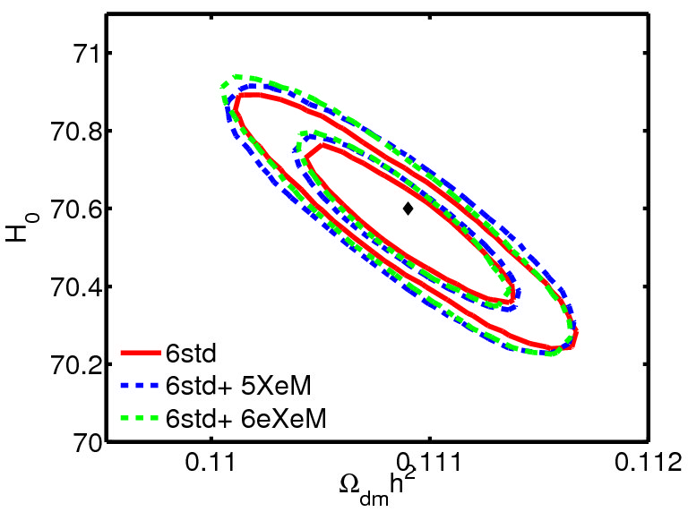
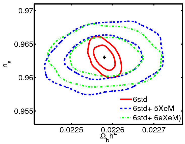
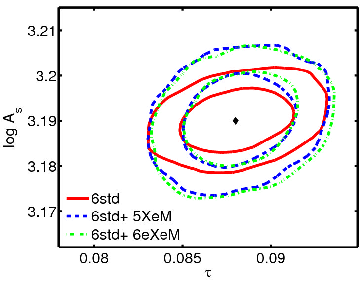
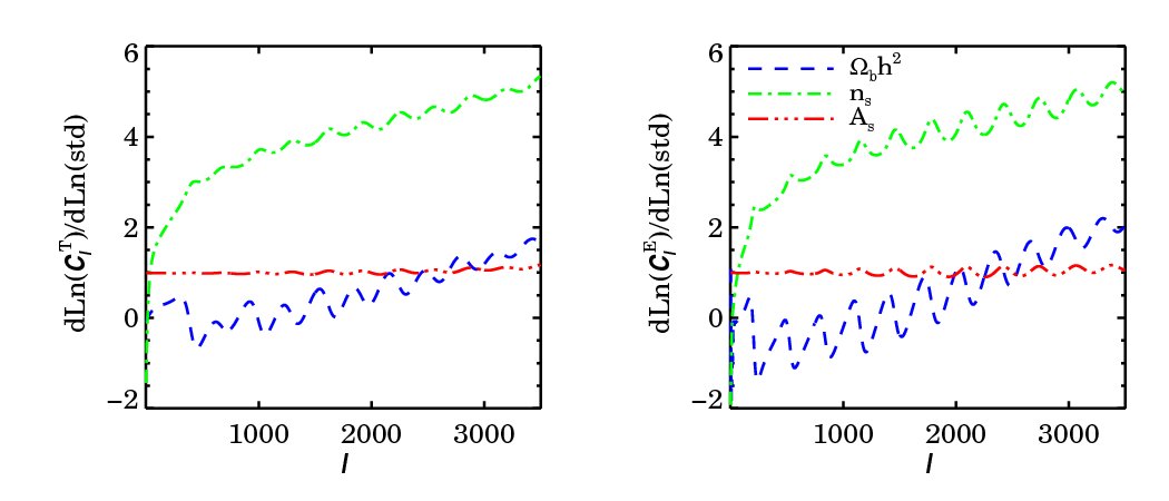
As the first example we choose the fiducial recombination model (here the SRS) to be identical to the ionization history used in the simulation of the data. We ran CosmoMC to estimate the best-fit values and errors of the six standard parameters together with those for the perturbation eigenmodes. We tried the two sets of eigenmodes described before: the first five XeMs and the first six eXeMs. The number of modes in each case was chosen in rough agreement with the mode cutoffs described in § 3.10. The simulations were carried out for a CVL experiment.

Figure 18.— The contours for the standard parameters as measured by an ideal experiment in the presence of five (six) XeMs (eXeMs) compared to the case with no eigenmodes included. The input value of the parameters is shown by the black diamond.

Figure 19.— The derivatives of the $C_{\ell}^{T,E}$’s with respect to some of the standard parameters.

Table 5The standard deviations of the first five XeMs from chains produced by CosmoMC, marginalized over the main six standard parameters.

XeM	1	2	3	4	5
$1\sigma$	0.046	0.030	0.057	0.088	0.086

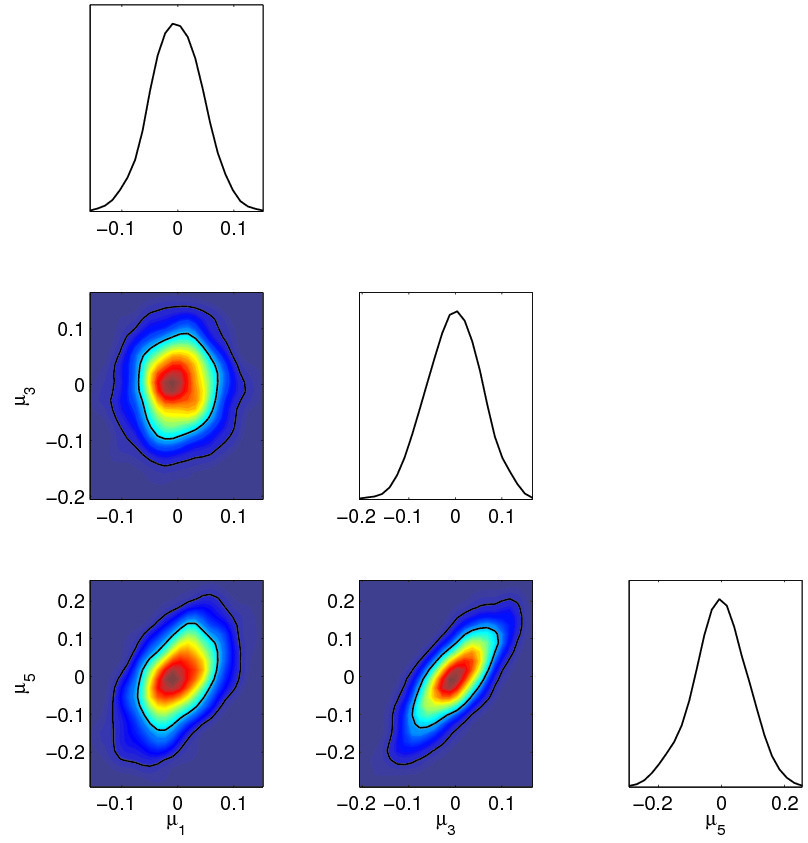
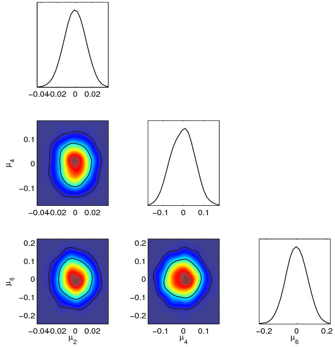
One expects no detection of eigenmodes since the fiducial model for ${X_{\rm e}}$ and the underlying model used to simulate data are the same, as verified by Figs. 16 and 17. Also, by construction there is almost no visible correlation between the measured parameters for the eXeMs, at least sufficiently close to the best-fit model where the assumptions of the Gaussianity for the likelihood surface approximately holds. However, Fig. 16 indicates that the XeMs become partially correlated with each other, although by construction these were initially uncorrelated . The reason is that the standard parameters were held fixed during the process of XeM construction, but now that they are allowed to vary, their degeneracy with the XeMs induces correlations. These new correlations lead to larger errors than those deduced from the simple Fisher analysis (Table 1 cf. Table 5) and can also change the rank ordering of the modes, e.g., the error on XeM 2 is smaller than XeM 1 (Table 5).

The standard parameters remain unbiased, as the model used for simulating data and the theoretical model used in the analysis were the same. This is no longer true once recombination corrections to the SRS are added (see Fig. 20). However, the correlations of the eigenmodes with some of the standard parameters increase the errors of the standard parameters. From Fig. 18 we see that among the standard parameters, $\Omega_{\rm b}h^{2}$, $n_{\rm s}$ and $A_{\rm s}$ are the ones most affected by the introduction of the eigenmodes into the analysis. This can be understood by noting the relatively high degeneracy between these parameters and some of the eigenmodes. The most evident one is the correlation of $n_{\rm s}$ with the first XeM which by changing the width of the visibility function leads to a tilt in the power spectra (compare Figs 19 and 11). For the case of $\Omega_{\rm b}h^{2}$ and $A_{\rm s}$ it is harder to give a visual interpretation. $\Omega_{\rm b}h^{2}$, leading to both tilt changes and oscillations in the $C_{\ell}$’s, correlates with most of the first five XeMs (the highest being with XeM 1), while $A_{\rm s}$, being an amplitude multiplier, mainly correlates with XeM 1. These correlations between the standard parameters and the eigenmodes emphasize the fact that uncertainties in the recombination scenario in particular undermine our ability to measure the precise values of $n_{\rm s}$ and $\Omega_{\rm b}h^{2}$ (see e.g., Shaw & Chluba, 2011). Also note that the changes in the error bars of the standard parameters are actually practically independent of which set of eigenmodes are used (Fig. 18). This suggests that in terms of the standard parameter estimation, the use of XeMs or eXeMs should not lead to vastly different results in the parameter estimation. However, the perturbations are measured to higher accuracy with the eXeMs (Table 3) than XeMs (Table 5) especially if only a few modes are included in the analysis. Therefore, as long as only CMB data are used, the eXeMs are the more appropriate choice of eigenmodes.

Table 6$Y_{\rm p}$ and its measured error from simulations for a CVL and a Planck-ACTPol-like experiment, with XeMs and eXeMs taken into account as perturbation eigenmodes, compared to the case with no eigenmodes.

	CVL(std)	Planck-ACTPol(std)	CVL(std + 5 XeMs)	CVL(std + 6 eXeMs)	Planck-ACTPol(std + 3 XeMs)
$Y_{\rm p}$	$0.240\pm 0.0016$	$0.240\pm 0.006$	$0.239\pm 0.005$	$0.240\pm 0.004$	$0.238\pm 0.017$

Figure 20.— Contours of some of standard parameters for CT2010 case, with eight XeMs in one case and 20 eXeMs in the other case included in the analysis, compared to a case where no perturbation eigenmodes (of any kind) has been included (the solid red curves). The simulations are performed for a CVL experiment. The input value of the parameters is shown by the black diamond.

Figure 21.— Similar to Fig. 20 but for a Planck-ACTPol-like experiment. Here three eigenmodes were added for both the XeM and eXeM case.

Finally, we studied how much the presence of perturbations to recombination could affect our ability to determine the precise value of $Y_{\rm p}$. The abundance of helium affects the CMB anisotropies mainly because more helium implies fewer free electrons during hydrogen recombination. Consequently, $Y_{\rm p}$ should also couple significantly to the perturbation eigenmodes. We therefore performed simulations in which $Y_{\rm p}$ was also allowed to vary. The analysis was performed with three and five XeMs in the Planck-ACTPol-like and CVL case, and with six eXeMs for the simulated CVL data. Table 6 compares the $1\sigma$ error bars on $Y_{\rm p}$ in these cases. We see that for the CVL case similar number of XeMs and eXeMs used as the eigenmodes lead to similar constraints on helium abundance. However, a Planck-ACTPol-like observation gives a few times larger error due to lack of very high sensitivity to very small scales, although fewer XeMs compared to the CVL case have been used.

4.2. Case 2: A perturbed recombination scenario

As the second example of parameter estimation and perturbation reconstruction, we simulate data assuming the recombination calculation of CT2010 (Fig. 10), while we take the fiducial model to be as of Recfast v1.4.1 or older (equivalent to SRS with ${\rm He_{switch}}=0$, to remove the helium correction which has been assumed as part of the perturbations in the data). The purpose here is to find out how well the biases in the standard parameters due to this lack of knowledge about the physical corrections can be removed by including the perturbation eigenmodes, and whether or not, data can reconstruct part of the true recombination history.

Constructed from CosmoMC chains for a CVL experiment, Fig. 20 illustrates the $2$D-contours of some of the standard parameters. The large biases in the estimated values of the parameters when only the six standard parameters are measured is due to the mismatch between the ionization histiry in the theoretical model and the data. Here only contours for parameters with the largest biases are shown. See also Shaw & Chluba (2011). To compensate for this mismatch we separately add to the parameters the two different sets of the eigenmodes, the XeMs and eXeMs, as the new parameters.

As Fig. 20 demonstrates, this eliminates the biases in the standard parameters, however, at the cost of increased error bars. In particular for $\Omega_{\rm b}h^{2}$ the difference is large. The error (corresponding to $\sim 5\sigma$ without eigenmodes) increases by a factor of $\sim 5$ when the (e)XeMs are included. For $n_{\rm s}$, similarly, the error (of $\sim 7\sigma$) decreases by a factor of 2. Also for $A_{\rm s}$ we find a similar degradation, while for $\tau$ the difference is rather small.

Our computations indicate that with the XeMs as the eigenmodes and for a CVL observation, the minimum number of modes required to remove the bias from these standard parameters is six. However, we included eight modes in the analysis to take into account the mode-selection criterion of § 3.10 (determined by the relative injection jumps).

We also observe that the recovered values for the amplitude of the XeMs are biased (compared to the theoretically expected values from direct projection on the XeMs, Table 2), and change by varying the number of modes included in the analysis. That is due to the correlation of the XeMs in the presence of the standard parameters, and the fact that not all XeMs are included into the parameter estimation. As a results, parts of the perturbation that project on the neglected higher XeMs leak into the lower XeMs. The bias in the measured XeM amplitudes is similar to the bias in the standard parameters when there are no eigenmodes in the analysis, but with a much lower significance.

For the same reason, the errors on the XeMs also change when the number of modes included in the analysis changes. However, as mentioned before, due to the low significance of the perturbation detection for most of the XeMs this is not as important as for the main cosmic parameters. For the CVL simulations with six and eight XeMs included, we see that the most significant contribution comes from the first mode (respectively $\mu_{1}=-0.23\pm 0.05$, $\mu_{1}=-0.18\pm 0.04$) while the other modes are consistent with zero. This is also true for a Planck-ACTPol-like case, which we will come to shortly, where the first XeM is measured to be $\mu_{1}=-0.22\pm 0.06$ $\mu_{1}=-0.24\pm 0.12$ for one and three XeM measurements.

Figure 22.— Left: The $\delta{X_{\rm e}}/{X_{\rm e}}$ as measured by a CVL experiment by including eight XeMs (and six standard parameters) in the analysis. The colors show the density of trajectories going through each point in the $z$-$\delta{X_{\rm e}}/{X_{\rm e}}$ space, normalized to one at each $z$. The maximum and $1$ and $2\sigma$ widths of the Thomson visibility function have been marked at the bottom of the plot. As this plot and the next ones indicate, the main recovery of ${X_{\rm e}}$ is the slope of the cure around this visibility peak. Middle and right: similar to the left figure, but for $\delta C_{\ell}^{TT,EE}/C_{\ell}^{TT,EE}$ trajectories.

Figure 23.— Similar to Fig. 22 but with the first ten eXeMs.

Figure 24.— Similar to Fig. 22 but with the first twenty eXeMs. As this figure demonstrates, including a higher number of modes does not necessarily lead to better ${X_{\rm e}}$ recovery. Here the recovered ${X_{\rm e}}$ becomes noisier compared to the case with only ten modes included, while the $C_{\ell}$ trajectories do not change significantly except for the diminished oscillations around the input model, as discussed in the text.

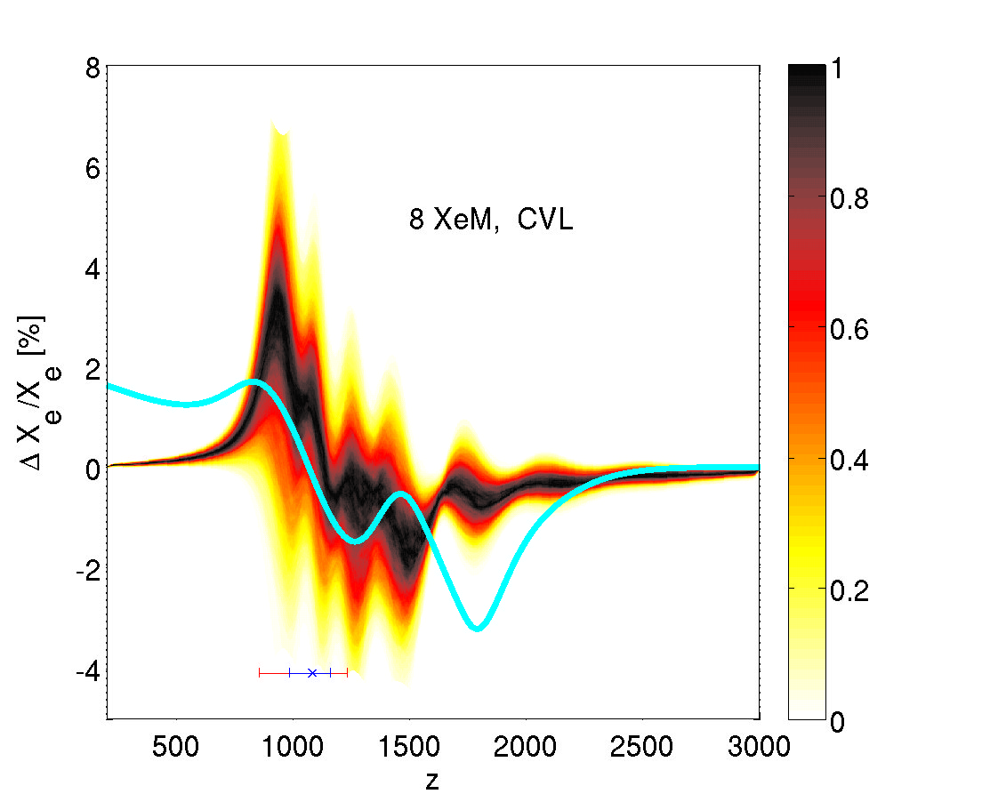
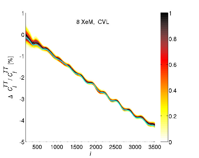
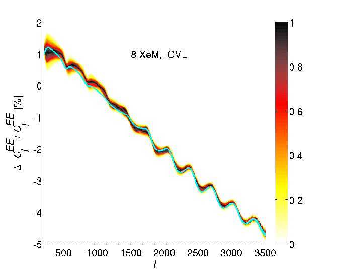
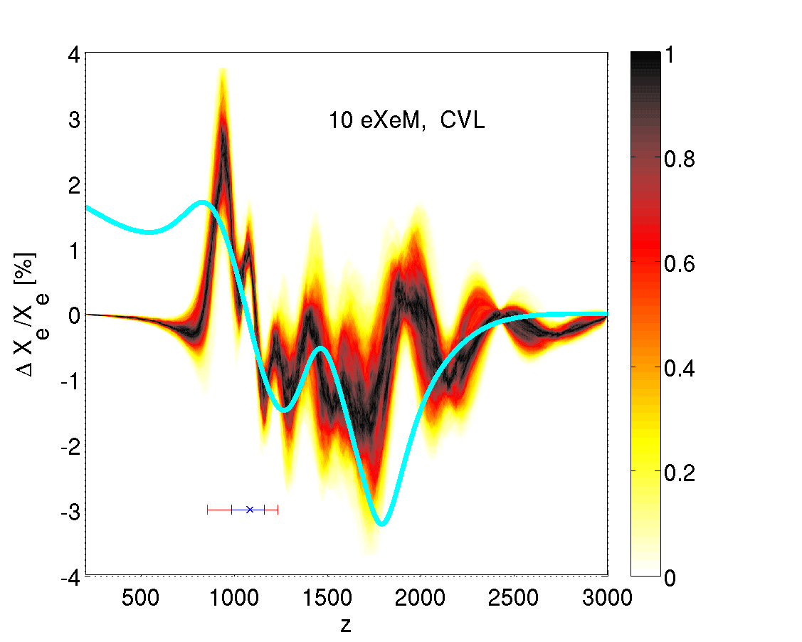
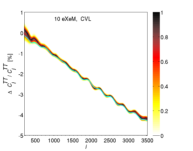
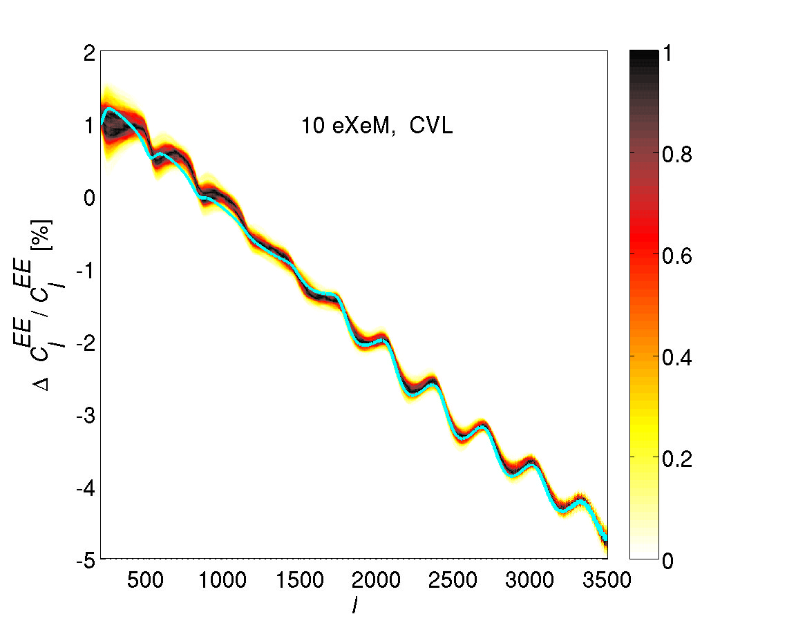
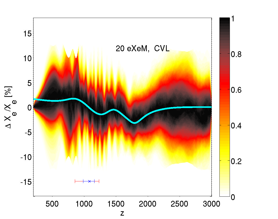
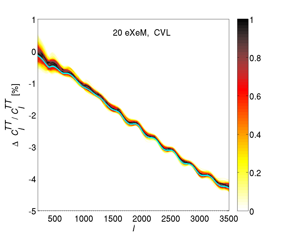
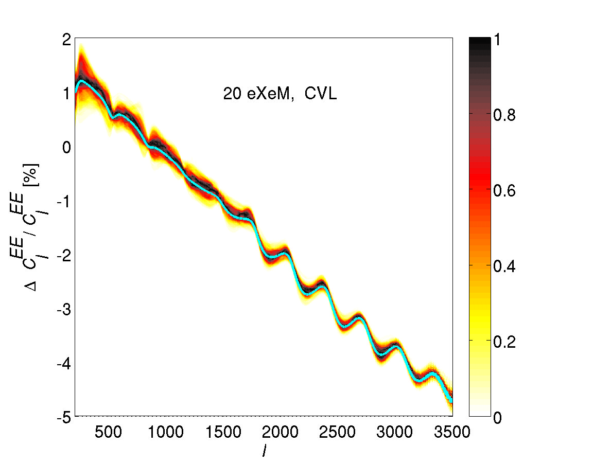
If instead eXeMs are used as the perturbation eigenmodes, our computations show that at least ten modes should be added to get rid of the bias for a CVL case. However, as a test case, we tried including the best 20 eXeMs (see Fig. 20).

We also found that although the errors on the standard parameters keep increasing by adding more eXeMs to the analysis up to around the tenth mode (which is required to remove the bias) it stays more or less the same afterwards. This suggests that in terms of the constraints on the standard parameters, we do not lose much by increasing the number of eXeMs. Besides, including more eXeMs does not affect the measurement of the previously included eigenmodes, as they are by construction uncorrelated (in the presence of standard parameters). Including more eXeMs, on the other hand, makes the reconstructed perturbations closer to the input model of perturbations (as in Fig. 10). However, as the errors of modes increase by going to higher orders, the error on the reconstructed curve increases. We will address this point in the next section.

Among the first 20 eXeMs for a CVL experiment, the modes with the most significant contributions (i.e., with at least $1\sigma$ detection) are $\mu_{2}=0.11\pm 0.02$, $\mu_{3}=0.10\pm 0.03$, $\mu_{9}=-0.31\pm 0.16$ and $\mu_{11}=-0.36\pm 0.24$ (compare to their theoretical prediction from direct projection of the perturbations on the eXeMs: $\mu_{2}=0.14$, $\mu_{3}=0.10$, $\mu_{9}=-0.33$ and $\mu_{11}=-0.39$). The reason that the recovered value, though close, is not exactly the same as the forecast is that the assumption of the Gaussianity of the distributions of the eXeMs and the standard parameters is only approximate. Also the eigenmodes have been slightly smoothed in the construction process which may cause numerical inaccuracy and induce slight correlation between the smoothed modes. By comparing the theoretical values of projection of the perturbation on the eXeMs and their forecast errors (from Fisher analysis) we do not expect any perturbation detection after eXeM 11.

Fig. 21 shows similar contours but for a simulated Planck-ACTPol-like observation. For the analysis we used the eigenmodes (both eXeMs and XeMs) constructed with the Planck-ACTPol simulated noise. The results from the two sets of eigenmodes are very similar. For both XeMs and eXeMs, one mode was sufficient to remove the bias ($\mu_{1}=-0.22\pm 0.06$ and $\mu_{1}=-0.20\pm 0.06$ respectively). This happens to be in agreement with the cutoff mode for the XeMs while with the eXeMs the second mode should also be included. The lower number of modes required for the Planck-ACTPol-like case compared to the ideal experiment is expected due to higher sensitivity of the data in the latter to deviations from the underlying ${X_{\rm e}}$ history. We also tried three modes, with no significant detection of the new modes, while the error on the XeM 1 increases by a factor of 2.

4.3. Trajectories

In this section we investigate the reconstruction of the ${X_{\rm e}}$-perturbations using the simulated data to illustrate the corresponding uncertainty at different redshifts. The left plot in Fig. 22 shows the redshift interval covered by $500$ $\delta\ln{X_{\rm e}}$-trajectories corresponding to an ideal observational case with eight XeM included, for the CT2010 model. The color indicates the number of trajectories passing through each $(z,\delta{X_{\rm e}}/{X_{\rm e}})$ bin, normalized to one at each redshift snapshot. The trajectories clearly show deviations from the SRS, slowly morphing into the correction obtained by CT2010 (the cyan curve). However, the recovery is not perfect, as the model of CT2010 has non-zero (and relatively significant) projection on higher XeMs which are not well constrained by data, and therefore were not included into the analysis. Most obviously, corrections to helium recombination are not captured well when using only the first few XeMs. These trajectories do not recover the analytical projection of the CT2010 corrections on the first eight XeMs very well either. The reason, as discussed before, is that the correlation of the XeMs induced by the standard parameters draws some contribution from the higher absent modes which biases the measurement of the first few XeMs included in the measurement.

To test this impact of higher, excluded modes on the recovered (low XeM) trajectories, we ran simulations with the data that only accounted for the contributions from these low modes. As expected, in the absence of higher modes in the data, the measured XeMs were non-biased and thus the highest probability region of the trajectories covered the $\delta\ln{X_{\rm e}}$ curve of the input model.

Although our basic target is ${X_{\rm e}}$-recovery, the relevant space for determining how well we have done is that of the CMB data, reduced to the power spectra, $C_{\ell}^{TT}$ and $C_{\ell}^{EE}$. The central and right panels of Fig. 22 show the $\delta C_{\ell}^{TT}/C_{\ell}^{TT}$ and $\delta C_{\ell}^{EE}/C_{\ell}^{EE}$ trajectories, where $\delta C_{\ell}^{X}/C_{\ell}^{X}=(C_{\ell}^{X}-C_{\ell}^{X,{\rm fid}})/C_{\ell}^{X,{\rm fid}}$ and $C_{\ell}^{\rm fid}$ is the fiducial power spectrum without any perturbations. The transformation from ${X_{\rm e}}$ trajectories to $C_{\ell}$ trajectories shows a much tighter band around the input signal. This is a visual confirmation of the point that some features in the $\delta\ln{X_{\rm e}}$ which make the ${X_{\rm e}}$ trajectories thick do not leave a measurable imprint on the $C_{\ell}$’s. Notice there are small residual oscillations. They coincide with the peaks and troughs of the $C_{\ell}$ curves for both $TT$ and $EE$ (which is out of phase with $TT$). One source for the oscillations seems to be the eigen mode truncation, as we will see later. Using only a limited number of the modes in the analysis causes the non-${X_{\rm e}}$ cosmic parameters to try to match the injected ${X_{\rm e}}$ perturbations. There is also an issue of accuracy of the $C_{\ell}$ code for some of the distortions.

Figure 25.— Similar to Fig. 22 but for a Planck-ACTPol-like experiment and with only three XeMs taken into account.

Figure 26.— Similar to Fig. 23 but for a Planck-ACTPol-like experiment and with only three eXeMs taken into account.

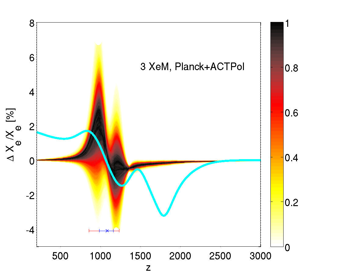
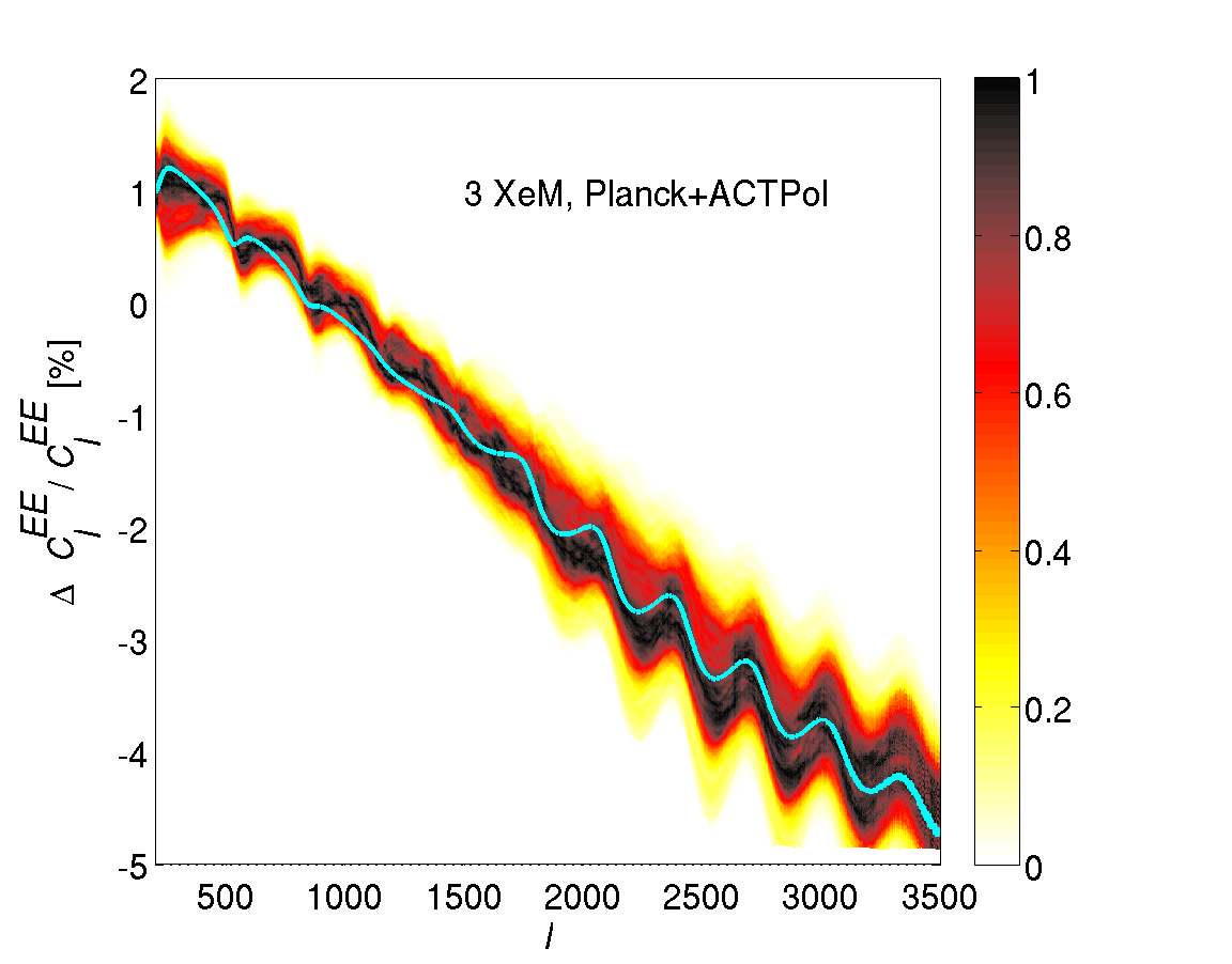
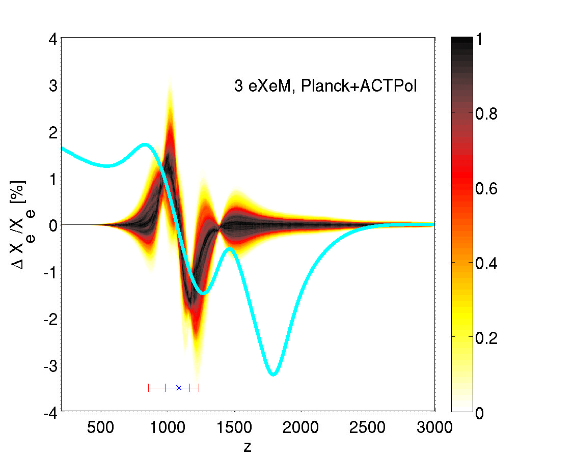
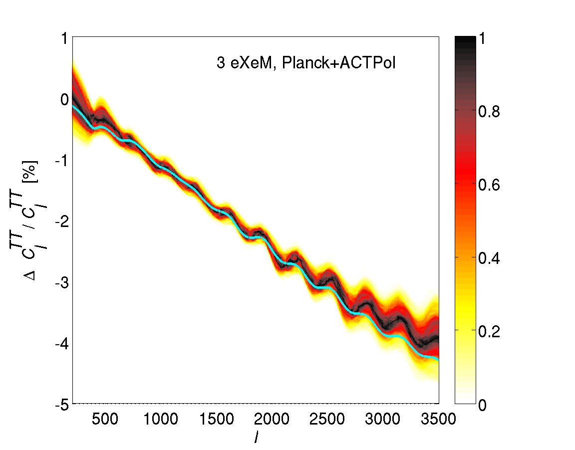
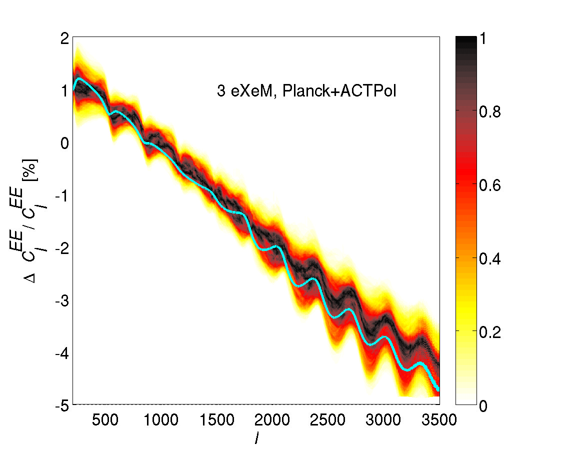
Fig. 23 similarly shows the $2$D histograms of trajectories for the case with the first ten eXeMs included. Around the maximum of the Thomson visibility function the ${X_{\rm e}}$ reconstruction is slightly stronger and less fuzzy than in Fig. 22, with part of the helium recombination correction being recovered. The improvement in the reconstruction is because for the computation of these eigenmodes their correlation with the standard parameters have been optimally taken care of. In contrast, the XeMs used in the previous case are non-optimal if no strong additional priors can be placed on the standard parameters, leading to confusion in the errors and the rank-ordering of the modes. Fig. 24, constructed with 20 eXeMs included, shows that the oscillation effect mentioned above around the input $C_{\ell}$ signal is diminished (and also partially swamped by the slightly higher dispersion around the input curve) for the 20-mode compared to the ten-mode case. We also see that including a higher number of modes does not necessarily lead to better ${X_{\rm e}}$ recovery.

Similar trajectories for a Planck-ACTPol-like experiment are shown in Figs. 25 and  26, with three XeMs and three eXeMs as the eigenmodes respectively. The trajectories for the XeMs are more widely spread and blurred due to experimental noise. The eXeMs perform slightly better. However, the overall reconstruction is clearly lacking detailed agreement with the full recombination correction of CT2010. In particular, most of the modification during helium recombination is not captured, as the corresponding signals can only be picked up with higher modes, which in the considered case are not constrainable at a significant level. In the $\delta C_{\ell}/C_{\ell}$ plots of these Planck-ACTPol-like cases, there is a small disagreement at high multipoles between the theoretical curve and the highest probability region of the chains. That is mainly due to mode truncation at a relatively low mode number, i.e., three. We tested this by including eight modes and as expected, observed a wider spread around the input signal with the disagreement diminished.

Although we do not plot the equivalent $\delta C_{\ell}/C_{\ell}$ for the DM case discussed in § 3.5.2, very similar plots result, namely good recovery of the power spectra with a dispersion around the input perturbation signal.

4.4. Beyond small perturbations

In this paper it was explicitly assumed that the model best explaining the ionization fraction (or the true model underlying the ionization history) is only slightly different from our fiducial model, justifying our choice of parameter $\delta\ln{X_{\rm e}}$. Therefore, the eigenmodes constructed for the fiducial model are also very close to the eigenmodes for the perturbations to the true ${X_{\rm e}}$, the corrections to the eigenmodes arising from the difference between the fiducial and true ${X_{\rm e}}$ model being only of second order. Under this assumption, a one step search for the best-fit parameters suffices to extract the available relevant information from the data, provided that the minimum required number of modes are included in the analysis. Finding the minimum number of required modes can by itself involve several parameter estimation steps in parameter spaces with different dimensions, the criterion being that the best fit values for the standard parameters stop changing. That is what was done in the examples in this work (§ 4.2), to illustrate how the method works.

However, if the fiducial model is very far from the true ${X_{\rm e}}$ history, such that the eigenmodes are expected to be affected at a significant level, an iterative approach toward finding the best modes with their associated amplitudes and errors is required: starting with our best guess for the fiducial model, we estimate its deviation from the true ionization history using the dataset available and the eigenmodes constructed based on this fiducial model. We then update the model by adding to it the measured deviations in the eigenmodes (and the standard parameters, if required). This process is repeated until the convergence of the model and its eigenmodes.

However, current constraints seem to indicate that such an iterative procedure will not be necessary within the standard picture. For example, as shown by Shaw & Chluba (2011), the recombination corrections of CT2011 are readily incorporated using one calibrated redshift dependent correction function relative to the original recombination model of Seager et al. (1999). Even for CVL errors a second update of the correction functions leads to minor effects. Nevertheless, if something more surprising occurred during recombination, an iterative approach might be required.

5. conclusion and discussion

CMB data today are becoming so precise that small modifications in standard ionization history are important. This impressive progress not only implies that measurements of the main cosmological parameters are becoming increasingly accurate, but also means that remaining uncertainties in the recombination dynamics, e.g., caused by neglected standard or non-standard physical processes, should be quantified. In this work we discuss a novel approach to constrain this remaining ambiguity with future CMB data. We performed a principal component analysis to find parameter eigenmodes that can be used to describe uncertainties in the ionization fraction. We constructed ${X_{\rm e}}$ eigenmodes over the redshift range of $[200,3000]$, performing several consistency checks to prove the correctness of our method. This approach automatically delivers a hierarchy of mode functions that can be selected according to their error and then are added to the standard cosmological parameters when analyzing CMB data.

Due to the strong CMB signal imprinted by hydrogen recombination, the most constrained modes are mainly localized around $z\sim 1100$, with some extensions to lower and higher redshift regions (see Fig. 4 and 12). This emphasizes that CMB data are very sensitive to small changes during hydrogen recombination, while details of helium recombination or small changes in the freeze-out tail are hard to constrain, unless strong priors on the reliability of the hydrogen recombination model are imposed. With the method described here it is possible to construct mode functions for different experimental situations, also folding in prior knowledge on the recombination history using appropriate weight functions and fiducial ${X_{\rm e}}$ models. For example, if there are physically motivated and experimentally supported hints toward (significant) changes in the freeze-out tail of recombination, e.g., due to energy injection from dark matter annihilation, we propose a parametrization which weights the low redshift part more strongly (see Fig. 9).

After we completed this work, we received a preprint (Finkbeiner et al., 2011) which investigated the use of CMB data to constrain details of energy injection scenarios related to decaying or annihilating particles. They also used parameter eigenmodes, but these were constructed based on an energy release history which is in our language akin to the imposition of a strong prior on the recombination dynamics around $z\sim 1100$ and a focus on the freeze-out tail of the recombination.

We applied the method to different simulated datasets with the aim to assess how well future CMB experiments will be able to constrain modifications to the standard recombination scenario. (Current WMAP plus ACT and SPT data will provide only relatively weak constraints, but Planck plus ACTPol and SPTPol will considerably improve the situation.) As a working example we used the refined recombination calculations of CosmoRec. For simulated CMB datasets corresponding to Planck-ACTPol-like experiments we found that the first 3 eigenmodes can be rather well constrained. The addition of these modes allows us to partially morph from the old Recfast ${X_{\rm e}}$ model to the new recombination history computed with CosmoRec without actually directly using the recombination corrections in the analysis. However, because the first few mode functions are strongly localized around $z\sim 1100$ details during helium recombination and in the freeze-out tail are not captured (Fig. 26). The addition of the first 3 eigenmodes is sufficient to remove the biases in the standard parameters, however, at the cost of increased error bars. We also show that for CVL limited experiments up to $l\sim 3500$ up to 10 modes might be constrainable, in this case allowing us to pick up part of the details during helium recombination (Fig. 23).

The significance of the detection of any perturbation obviously depends on the underlying ionization history of the real data. In the specific CosmoRec example for Planck-ACTPol-like experiments, all three modes but the first one are consistent with zero. A significant source for large errors on the eigenmodes is their correlation with the standard parameters. If tight constraints are imposed on the standard parameters by non-CMB experiments such as BAO or SN data, the errors on the eigenmodes will be correspondingly reduced. Comparing the first rows of Table 1 (where all standard parameters are held fixed) and Table 3 (where all standard parameters are being marginalized over) illustrates the effect of this correlation in the extremes.

This also shows how important one’s knowledge in how well elements of recombination are known, expressed through prior probabilities, will be. If the uncertainty in the ionization history during hydrogen recombination can be reliably reduced by other methods then the sensitivity to small perturbations at higher or lower redshifts is enhanced. We note that measurements of the cosmological recombination radiation (e.g., see Chluba & Sunyaev, 2006a; Sunyaev & Chluba, 2009) could in principle provide an alternative way of constraining the recombination dynamics in the future. In particular, the recombination radiation could exhibit significant features if something more unexpected occurred during different cosmological epochs (e.g., see Chluba & Sunyaev, 2009; Chluba, 2010).

In principle, for a complete study of ionization history, late reionization should also be included in the analysis. Ambiguities in the low redshift part of the ionization history may affect the measurements of high redshift perturbations and vice versa. However, the main signal from the reionization epoch is measurable from the very large scale CMB polarization, and the high redshift perturbations of ${X_{\rm e}}$ affect anisotropies with smaller angular scales. Therefore the signals from these two regions are rather uncorrelated. A more complete analysis for the whole ionization history or where different parts of it are considered simultaneously is for future work.

An aspect requiring decision when analyzing real data is the choice of parametrization. For most of this work we weighted the perturbations in ${X_{\rm e}}$ by the fiducial history. If, for example, the recovered perturbations point towards modifications in the freeze-out tail of recombination, or if there is strong belief that no sign of significant deviations around the maximum of visibility are present, an alternative parametrization which allows better reconstruction of the tail can be constructed, using appropriate weight functions that quantify our belief in the underlying fiducial model.

As discussed in § 4.4, our semi-blind XeMs are designed to only probe small perturbations about the fiducial model ${X_{\rm e}^{\rm fid}}$. When it comes to real CMB data analysis, iterations of ${X_{\rm e}^{\rm fid}}$ are required to ensure no leftover bias remains. We look forward to the application of iteratively-improved eigenmodes to the coming high resolution CMB data from Planck, ACTPol and SPTPol.

We thank Doug Finkbeiner, Tongyan Lin and Olivier Doré for useful discussions and Eric Switzer for his comments on the text. Support from NSERC and the Canadian Institute for Advanced Research is gratefully acknowledged.

References

- Ali-Haïmoud & Hirata (2010) Ali-Haïmoud, Y., & Hirata, C. M. 2010, Phys. Rev. D, 82, 063521
- Ali-Haïmoud & Hirata (2011) —. 2011, Phys. Rev. D, 83, 043513
- Bond (1996) Bond, J. R. 1996, in Cosmology and Large Scale Structure, ed. R. Schaeffer, J. Silk, M. Spiro, & J. Zinn-Justin, 469–+
- Bond et al. (1997) Bond, J. R., Efstathiou, G., & Tegmark, M. 1997, MNRAS, 291, L33
- Chen & Kamionkowski (2004) Chen, X., & Kamionkowski, M. 2004, Phys. Rev. D, 70, 043502
- Chluba (2010) Chluba, J. 2010, MNRAS, 402, 1195
- Chluba & Sunyaev (2006a) Chluba, J., & Sunyaev, R. A. 2006a, A&A, 458, L29
- Chluba & Sunyaev (2006b) —. 2006b, A&A, 446, 39
- Chluba & Sunyaev (2008) —. 2008, A&A, 480, 629
- Chluba & Sunyaev (2009) —. 2009, A&A, 501, 29
- Chluba & Sunyaev (2010) —. 2010, MNRAS, 402, 1221
- Chluba & Thomas (2011) Chluba, J., & Thomas, R. M. 2011, MNRAS, 412, 748
- Das et al. (2011) Das, S., et al. 2011, ApJ, 729, 62
- De Boor (2001) De Boor, C. 2001, A Practical Guide to Splines (Springer-Verlag)
- Dubrovich & Grachev (2005) Dubrovich, V. K., & Grachev, S. I. 2005, Astronomy Letters, 31, 359
- Dunkley et al. (2010) Dunkley, J., et al. 2010, ArXiv e-prints
- Farhang et al. (2011) Farhang, M., Bond, J. R., Doré, O., & Barth Netterfield, C. 2011, ArXiv e-prints
- Fendt et al. (2009) Fendt, W. A., Chluba, J., Rubiño-Martín, J. A., & Wandelt, B. D. 2009, ApJS, 181, 627
- Finkbeiner et al. (2011) Finkbeiner, D. P., Galli, S., Lin, T., & Slatyer, T. R. 2011, ArXiv e-prints
- Fixsen (2009) Fixsen, D. J. 2009, ApJ, 707, 916
- Galli et al. (2009) Galli, S., Melchiorri, A., Smoot, G. F., & Zahn, O. 2009, Phys. Rev. D, 80, 023508
- Grin & Hirata (2010) Grin, D., & Hirata, C. M. 2010, Phys. Rev. D, 81, 083005
- Hajian et al. (2010) Hajian, A., et al. 2010, ArXiv e-prints
- Hirata (2008) Hirata, C. M. 2008, Phys. Rev. D, 78, 023001
- Hu & Holder (2003) Hu, W., & Holder, G. P. 2003, Phys. Rev. D, 68, 023001
- Hütsi et al. (2011) Hütsi, G., Chluba, J., Hektor, A., & Raidal, M. 2011, ArXiv e-prints
- Hütsi et al. (2009) Hütsi, G., Hektor, A., & Raidal, M. 2009, A&A, 505, 999
- Jentschura (2009) Jentschura, U. D. 2009, Phys. Rev. A, 79, 022510
- Kaplinghat et al. (1999) Kaplinghat, M., Scherrer, R. J., & Turner, M. S. 1999, Phys. Rev. D, 60, 023516
- Karshenboim & Ivanov (2008) Karshenboim, S. G., & Ivanov, V. G. 2008, Astronomy Letters, 34, 289
- Kholupenko & Ivanchik (2006) Kholupenko, E. E., & Ivanchik, A. V. 2006, Astronomy Letters, 32, 795
- Kholupenko et al. (2007) Kholupenko, E. E., Ivanchik, A. V., & Varshalovich, D. A. 2007, MNRAS, 378, L39
- Komatsu et al. (2011) Komatsu, E., et al. 2011, ApJS, 192, 18
- Labzowsky et al. (2009) Labzowsky, L., Solovyev, D., & Plunien, G. 2009, Phys. Rev. A, 80, 062514
- Lewis et al. (2000) Lewis, A., Challinor, A., & Lasenby, A. 2000, ApJ, 538, 473
- Lueker et al. (2010) Lueker, M., et al. 2010, ApJ, 719, 1045
- MacKay (2003) MacKay, D. J. 2003, Information Theory, Inference, and Learning Algorithms, 1st edn. (Cambridge: Cambridge University Press)
- McMahon et al. (2009) McMahon, J. J., et al. 2009, in American Institute of Physics Conference Series, Vol. 1185, American Institute of Physics Conference Series, ed. B. Young, B. Cabrera, & A. Miller, 511–514
- Mennella et al. (2011) Mennella, A., et al. 2011, ArXiv e-prints
- Mitra et al. (2010) Mitra, S., Choudhury, T. R., & Ferrara, A. 2010, ArXiv e-prints
- Monaghan (2005) Monaghan, J. J. 2005, Reports on Progress in Physics, 68, 1703
- Mortonson & Hu (2008) Mortonson, M. J., & Hu, W. 2008, ApJ, 672, 737
- Niemack et al. (2010) Niemack, M. D., et al. 2010, in Presented at the Society of Photo-Optical Instrumentation Engineers (SPIE) Conference, Vol. 7741, Society of Photo-Optical Instrumentation Engineers (SPIE) Conference Series
- Padmanabhan & Finkbeiner (2005) Padmanabhan, N., & Finkbeiner, D. P. 2005, Phys. Rev. D, 72, 023508
- Peebles et al. (2000) Peebles, P. J. E., Seager, S., & Hu, W. 2000, ApJ, 539, L1
- Peebles & Yu (1970) Peebles, P. J. E., & Yu, J. T. 1970, ApJ, 162, 815
- Planck HFI Core Team et al. (2011) Planck HFI Core Team et al. 2011, ArXiv e-prints
- Rubiño-Martín et al. (2010) Rubiño-Martín, J. A., Chluba, J., Fendt, W. A., & Wandelt, B. D. 2010, MNRAS, 403, 439
- Rubiño-Martín et al. (2008) Rubiño-Martín, J. A., Chluba, J., & Sunyaev, R. A. 2008, A&A, 485, 377
- Scóccola et al. (2009) Scóccola, C. G., Landau, S. J., & Vucetich, H. 2009, Memorie della Societ Astronomica Italiana, 80, 814
- Seager et al. (1999) Seager, S., Sasselov, D. D., & Scott, D. 1999, ApJ, 523, L1
- Seager et al. (2000) —. 2000, ApJS, 128, 407
- Seljak et al. (2003) Seljak, U., Sugiyama, N., White, M., & Zaldarriaga, M. 2003, Phys. Rev. D, 68, 083507
- Seljak & Zaldarriaga (1996) Seljak, U., & Zaldarriaga, M. 1996, ApJ, 469, 437
- Shaw & Chluba (2011) Shaw, J. R., & Chluba, J. 2011, MNRAS, 963
- Slatyer et al. (2009) Slatyer, T. R., Padmanabhan, N., & Finkbeiner, D. P. 2009, Phys. Rev. D, 80, 043526
- Sunyaev & Chluba (2009) Sunyaev, R. A., & Chluba, J. 2009, Astronomische Nachrichten, 330, 657
- Sunyaev & Zeldovich (1970) Sunyaev, R. A., & Zeldovich, Y. B. 1970, Astrophysics and Space Science, 7, 3
- Switzer & Hirata (2008) Switzer, E. R., & Hirata, C. M. 2008, Phys. Rev. D, 77, 083006
- Tauber et al. (2010) Tauber, J. A., et al. 2010, A&A, 520, A1+
- The Planck Collaboration (2006) The Planck Collaboration. 2006, ArXiv Astrophysics e-prints
- Vanderlinde et al. (2010) Vanderlinde, K., et al. 2010, ApJ, 722, 1180
- Wong et al. (2008) Wong, W. Y., Moss, A., & Scott, D. 2008, MNRAS, 386, 1023
- Wong & Scott (2007) Wong, W. Y., & Scott, D. 2007, MNRAS, 375, 1441
- Zhang et al. (2007) Zhang, L., Chen, X., Kamionkowski, M., Si, Z., & Zheng, Z. 2007, Phys. Rev. D, 76, 061301
- Zhang et al. (2006) Zhang, L., Chen, X., Lei, Y., & Si, Z. 2006, Phys. Rev. D, 74, 103519