Inverse anisotropic diffusion from power density measurements in two dimensions
Abstract
This paper concerns the reconstruction of an anisotropic diffusion tensor from knowledge of internal functionals of the form with for solutions of the elliptic equation on a two dimensional bounded domain with appropriate boundary conditions. We show that for and appropriately chosen boundary conditions, may uniquely and stably be reconstructed from such internal functionals, which appear in coupled-physics inverse problems involving the ultrasound modulation of electrical or optical coefficients. Explicit reconstruction procedures for the diffusion tensor are presented and implemented numerically.
1 Introduction
Coupled-physics modalities are being extensively studied in medical imaging as a means to combine high contrast with high resolution. Such imaging modalities typically couple a high-contrast low-resolution modality with a low-contrast high-resolution modality. In this context, Ultrasound Modulated Optical Tomography (UMOT) or Ultrasound Modulated Electrical Impedance Tomography (UMEIT) aim to improve the low resolution in the reconstruction of diffusion (in OT) or conductivity (in EIT) coefficients by perturbing the medium with focused or delocalized ultrasound when making measurements. We assume here that the electric potential in EIT and the photon density in OT are modeled by the following elliptic model
| (1) |
where is a subset in , where will equal in this paper, and where is a symmetric positive definite tensor. In the case of OT, equation (1) is an approximation of a more accurate model that takes into account absorption effects by adding a zeroth order term with in the left-hand side of (1). Whether this additional term can be handled with the present approach will be the object of future research. We also assume that the ultrasound perturbation of the medium and of the corresponding boundary (current) measurements allow us to stably reconstruct the power density of two solutions of (1) with prescribed boundary conditions, namely, the quantity over . How to obtain power densities in practice has been addressed in e.g. [1] using highly focused ultrasonic waves, and in e.g. [12, 7] in the context of synthetic focusing.
The main objective of this paper is the reconstruction of the symmetric tensor in (1) and in dimension from knowledge of internal measurements , where each corresponds to a different, properly chosen boundary illumination .
The isotropic case was analyzed in two dimensions in [10] and extended to three dimensions in [7] and to all dimensions and more general types of measurements of the form in [16]. The case of internal current densities of the form arises in current density impedance imaging, see e.g. [17] and [6] for a review and bibliography of recent results obtained in similar problems. Although the results in this paper also extend to general values of , we restrict ourselves to the case to simplify the presentation. Similar problems in dimensions and were also analyzed in a linearized context in [13]; see also the recent paper [14] on general linearized hybrid inverse problems.
This paper extends the analyzes in [16] to the case of two-dimensional anisotropic diffusion tensors. We show that with (or, in practice, in fact ) properly chosen illuminations, the measurements allow for a unique and stable reconstruction of the full anisotropic tensor . In particular, the internal functionals considered here do allow us to uniquely reconstruct the conformal structure (or normalized anisotropy tensor) , unlike the case of Dirichlet-to-Neumann boundary measurements as they appear in the Calderón problem, where can be reconstructed up to a push-forward by an arbitrary change of variables leaving each point on invariant [3].
More precisely, using the decomposition with , the anisotropy tensor can be reconstructed in an algebraic and pointwise manner, after which the quantity can be obtained in two possible ways, either via inverting two consecutive gradient (or, after taking divergence, Poisson) equations, or by inverting a strongly coupled elliptic system followed by a gradient (or Poisson) equation. The reconstruction of is similar to the case where is known up to multiplication by a scalar function. Since this problem has the same dimensionality as that of the reconstruction of an isotropic diffusion tensor (treated in [10, 7, 16]), only illuminations are necessary and the reconstruction can be done following the second step of the previously described approach. Although some of the techniques presented here generalize to higher dimensions, we restrict ourselves to the two-dimensional setting in this paper.
Finally, some numerical simulations confirm the theoretical predictions: both the isotropic and the anisotropic parts of the tensor can be stably reconstructed, with a robustness to noise that is much better for the former than the latter.
2 Statement of the main results
Let be an open, bounded, simply connected domain. Borrowing notation from [4], for , a real symmetric matrix belongs to if and only if it satisfies the uniform ellipticity condition
| (2) |
In the following, we consider the problem of reconstructing an anisotropic conductivity function where is fixed, from the knowledge of power-density measurements of the form
where for , the function satisfies the conductivity equation
| (3) |
The ’s are prescribed illuminations. We denote by the unique positive -valued function that satisfies the pointwise relation . Clearly, .
We first change unknown functions by defining for , the vector fields . The elliptic equation (3) thus reads
| (4) |
Furthermore, denoting the “curl” operator in 2D by where , the fact that implies that it is curl-free, that is,
| (5) |
The data become . We now decompose into
| (6) |
From the uniform bounds , it follows immediatly that .
Over any open, connected set , where two solutions satisfy the following positivity condition
| (7) |
we can derive the first important relation
| (8) |
We now orthonormalize the frame into a -valued frame , via a transformation of the form (or, in matrix notation , ), where is known from the data. For further use we denote and define the vector fields as
| (9) |
This orthonormalization can be obtained by the Gram-Schmidt procedure or by setting for instance. Since is -valued, we parameterize it with a -valued function such that . One is then able to derive the following second important equation by using (4) and geometric arguments:
| (10) |
where and are known from the data, and , where denotes the -th column of .
Reconstruction of the anisotropy :
We start by defining the set of admissible illuminations for some , by stating that a quadruple belongs to if the following conditions are satisfied for some constant :
| (11) | ||||
| (12) |
where solves (3) for . Condition (12), which is directly motivated by calculations later, expresses the fact that the relative variations of the volumes and differ at every point, which seems to be the condition that guarantees that our measurements are rich enough to “see” the anisotropy.
Condition (11) is rather easy to ensure by virtue of [4, Theorem 4], which guarantees that (11) holds as soon as both maps and are homeomorphisms onto their images. Based on a construction that uses Complex Geometrical Optics (CGO) solutions, we construct in the next lemma solutions that satisfy condition (12) under some regularity assumption on . This in turn guarantees that is not empty when is smooth enough.
Lemma 2.1.
Consider now , and let us denote and . Define two orthonormal frames , obtained after orthonormalization of , and . Taking the difference of equations (10) for each system, we obtain the algebraic equation
| (14) |
and is defined in (12). Both vector fields and are uniquely determined by the data, see below. Since is only described by two scalar parameters, equation (14) together with the condition (12) allow us to reconstruct these two parameters algebraically and in a pointwise manner. When orthonormalization uses the Gram-Schmidt procedure, and satisfy the following boundedness and stability inequalities for some constants :
| (15) | ||||
where and respectively come from and . We arrive at the following result:
Theorem 2.2 (Anisotropy reconstruction in 2d with ).
For , the measurements uniquely determine the tensor via the explicit algebraic equation (14). Moreover, for with and with the corresponding measurements for , and in the case where orthonormalization is done using the Gram-Schmidt procedure, the following stability statement holds:
| (16) |
for some constant .
Remark 2.3.
In practice, we have observed numerically that was enough to reconstruct if we chose of the form .
Reconstruction of or :
Once the anisotropy is known, the problem of reconstructing now has the same dimensionality as that of reconstructing an isotropic conductivity. It requires only internal functionals satisfying (7) in .
A first approach towards reconstructing consists in solving a gradient equation for the scalar quantities and then , the right-hand sides of which are successively known. If and are known throughout the domain’s boundary, one may take the divergence of said gradient equations instead and solve Poisson equations with Dirichlet boundary conditions.
Such an approach provides Lipschitz-stable reconstructions as is summarized in
Theorem 2.4 (Stability of , first approach).
A second approach consists in inserting the expression in equation (8) into the elliptic equation (3) and deriving a strongly coupled elliptic system for the unknown . In two dimensions, this system turns out to have a variational formulation with a coercive bilinear form:
| (18) |
It thus admits a unique solution in the following space (up to an additive -lifting of )
| (19) |
Using a Fredholm-type argument, we obtain that this solution is also stable with respect to changes in the data, as stated in the following result:
Proposition 2.5 (Stability of the strongly coupled elliptic system).
Once the couple is reconstructed throughout , one may reconstruct using (a modified version of) the gradient equation (8).
Theorem 2.6 (Stability of , second approach).
Let the conditions of proposition 2.5 be satisfied. Then the reconstructed determinants and satisfy the stability estimate:
| (21) |
The rest of the paper is structured as follows. We first derive equations (8) and (10) in section 3, which form the cornerstone of all subsequent derivations. Section 4 covers the three reconstruction algorithms mentioned above. Section 5 provides a proof of lemma 2.1 while section 6 concludes with numerical examples for each reconstruction algorithm.
3 Proof of equations 8 and (10)
3.1 Geometrical setting and preliminaries
In this section, we work on an open connected subset , over which satisfy the positivity condition (7). For a matrix with , and a scalar , we can define uniquely by taking the positive -root of each eigenvalue. Now, because is uniformly elliptic for any , the vector fields also form an oriented frame (denoted ). The measurements can also be represented as
| (22) |
From this assumption, one can deduce that any vector field can be represented by means of the formula
| (23) |
Both equations (22) and (23) only “see” up to a scalar multiplicative constant, thus these equations still hold if we replace by .
Finally, we give the following important relation (only valid when ) true for any :
| (26) |
3.2 Proof of the gradient equation (8)
The derivation relies on the analysis of the properties of the vector fields for . First notice that since is skew-symmetric, we have
Then, using the relation (26) with and the fact that ,
This means that the vector fields can be expressed using the representation (23) with :
| (27) | ||||
We now apply the divergence operator to (27). Together with the fact that and equation (4), and using the identity , we derive
Multiplying the last equation by , summing over and dividing by , we obtain
The first term is of the form (23) with and and thus equals . We obtain the second term of the r.h.s. of (8). The first term of the r.h.s. of (8) is obtained from the second one by expanding the term and using the product rule and identity (23) to obtain the term.
3.3 Proof of (10)
We now orthonormalize into a frame via the transformation , also written as
The matrix satisfies , also written as for . It can be constructed by the Gram-Schmidt procedure or by writing . With the ’s defined in (9), the following important identity holds
| (28) |
Therefore, starting from (8), we have
| (29) |
where we have used (28) in the last equality. Now, in order to derive equation (10), we must write the Lie bracket in two different manners.
On the one hand, writing in the canonical basis and using the identity , we have that
after renumbering indices properly. Moreover, in the parameterization we have
thus we obtain
| (30) |
On the other hand, we compute using (4). First, deriving a divergence equation for , and using the fact that (4) can be recast as , we have
| (31) |
where we have used (29) in the last equality. We now use the following 2d vector calculus identity
| (32) |
where for a matrix. With and , we have
so the first term in the r.h.s. of (32) is zero. Thus we have
where we have used the properties and . Combining (30) with the last r.h.s. yields (10).
4 Reconstruction procedures
This section is devoted to the reconstruction procedures. We first reconstruct the anisotropic part of the conductivity tensor and second reconstruct and .
4.1 Reconstruction of the anisotropy with or
Let us now consider a quadruple with possibly . Condition (11) ensures that the matrices and satisfy the positivity condition (7). Let us denote the -valued matrix obtained after Gram-Schmidt orthonormalization, parameterized by an angle function , and denote
For each pair of solutions, we have the equation
| (33) |
Taking the difference of both systems cancels the term , and we obtain equation (14), with vector fields
Now we claim that although the angle functions are unknown, is known from the data. Indeed, we have that
and then,
where both r.h.s. only depend on the data. As a result, the vector fields are completely known from the data .
Parameterization of and inversion:
The matrix is symmetric and has unit determinant and as such is characterized by only two scalar parameters. This is why equation (14) is enough to reconstruct it algebraically wherever or . We now parameterize as follows
| (36) |
where the second row is deduced from the first one by constructing a symmetric matrix with unit determinant. With and , equation (14) becomes
which can be rewritten as
| (43) |
and can therefore be inverted as
| (44) |
Proof of theorem 2.2.
The only important point is to show that is never zero. Since condition (12) is satisfied, then never vanishes over . Since , we have . Therefore, wherever , that is, nowhere in this case. Inequality (16) follows provided that the inequalities (15) hold in the Gram-Schmidt case, and the expressions (44) are smooth in the components of away from . ∎
Remark 4.1 (An unstable parameterization of ).
Another way (seemingly geometrically more meaningful) to parameterize is, for , to write
| (51) |
describes the anisotropy and locates the main axes of the ellipse. However, besides the fact that this representation is not injective (indeed we have ), the reconstruction of becomes unstable as approaches .
4.2 Reconstruction of
We now consider the problem of reconstructing from measurements, assuming that is known. We assume that the positivity condition is satisfied throughout the domain . We propose two approaches, which we analyse consecutively in the next two sections.
4.2.1 Reconstruction of
This approach consists in reconstructing and then using the gradient equations (10) and (8). We first isolate in (10) by writing
| (52) |
We thus require an expression for . In the case where was reconstructed in the previous section using the variables, we need to compute from knowledge of , which we do by first introducing a parameterization of similar to (36), called with . Then, equating the terms in the first row of both representations and , we obtain the relations
which, using the condition we invert as,
| (53) |
In the variables , we now obtain the following expression for the term :
| (58) |
Using (58) in (52) allows us to reconstruct via integrating the gradient equation (52) along curves (and assuming that is known at one point of the domain). Alternatively, if is known on the whole boundary, one may apply the divergence operator on both sides of (52) and solve a Poisson equation with Dirichlet boundary conditions.
On to the reconstruction of , we now use equation (8) in the frame to obtain:
| (59) |
whose r.h.s. is completely known. For its resolution, equation (59) may be simplified using a calculation similar to [16, Sec. 6.2]. To this end, we define for and compute
where we have used the facts that and . The matrices and are symmetric matrices that can be expressed in the following manner
| (60) | ||||
From this we deduce the final expression of :
| (61) | ||||
Proof of Theorem 2.4.
The proof is very similar to [7, Theorem 3.2]. For two sets of measurements and , the error function on satisfies
Assuming that for some and using Gronwall’s lemma along (bounded) paths joining any to , and provided that in the Gram-Schmidt case, we arrive at the inequality
| (62) |
Similarly, using the difference of equation (59) for and and using (62), we arrive at (17). ∎
4.2.2 Reconstruction of
This approach, first introduced in [16], consists in writing a strongly coupled elliptic system for the unknowns , whose properties are particularly appealing in two dimensions. We proceed as follows.
In the frame , equation (8) reads
| (63) |
Now, the diffusion equation (3) can be rewritten as
Plugging (63) into the latter equation and using the fact that yields the system
| (64) | ||||
| (65) |
Upon multiplying (64) by and summing over , we obtain an equivalent formulation in divergence form
| (66) |
We assume that and define to be a -lifting of inside . Defining the new unknown , satisfies the following two equivalent systems whenever satisfies (64) or (66) and vice-versa
| (67) | |||
| (68) |
System (68) allows us to establish existence and uniqueness of while (67) is used to establish the stability of with respect to the data .
Uniqueness of :
System (68) can be recast as the variational problem of finding such that for every , we have
| (69) |
With endowed with the norm , assuming the positivity condition (7), the matrices , and are all uniformly elliptic over , which guarantees that the bilinear form is coercive. The continuity of and of the linear form over are straightforward. As a result, Lax-Milgram’s theorem establishes existence and uniqueness of solving (68) and (67), and thus of solving (64) and (66).
Stability of with respect to the data:
Let us define the operator , where is the unique solution to the problem
| (70) |
Since is uniformly elliptic, the operator is bounded (see e.g. [11]), thus compact by the Rellich compactness theorem. Therefore, applying to (67), we obtain the integro-differential system
which in vector notation may be recast as
| (71) |
Similarly to [16, Lemma 5.1], the operator is compact and its operator norm satisfies
| (72) |
see [16] for details. Therefore, equation (71) is a Fredholm equation and the boundedness of holds as soon as is not an eigenvalue of . This is the case here, since the previous paragraph proves exactly this fact. On to the stability of w.r.t. the data , we use the fact that the vector fields defined in (65) satisfy estimates of the form
whenever and have their components in and satisfy the positivity condition (7). With the previous estimate, the proof of proposition 2.5 is similar to [16, Proposition 2.6] so we do not reproduce it here.
Reconstruction of :
On to the reconstruction of , equation (63) can be recast as
| (73) |
the r.h.s. of which is now completely known. One may thus choose to solve this equation either solving ODE’s along curves or taking divergence on both sides and solving a Poisson equation. The stability of such a reconstruction scheme was already stated in theorem 2.6, whose proof may be found in the very similar (isotropic) context of [16, Theorem 2.8].
5 Proof of lemma 2.1
Isotropic case :
Consider the problem on with extended in a continuous manner outside of and such that equals outside of a large ball. Let on . We assume that , which holds if for some , i.e., the original . Note that by Sobolev imbedding, is of class while is of class .
Let so that on . Let be of the form with and so that , and . Thus, satisfies and is a harmonic complex plane wave. Now, it is shown in [8], following works in [9, 18], that
| (74) |
with and hence in . Furthermore, with the assumed regularity, [8, Proposition 3.3] shows the existence of a constant such that
| (75) |
Taking gradients of the previous equation and rearranging terms, we obtain that
| (76) |
Note that is complex-valued and since is real-valued, both the real and imaginary parts and are solutions of . More precisely, we have
| (77) | ||||
We now denote , and straightforward computations lead to
where . Letting so large that , the function is now bounded away from zero over . Taking logarithm and gradient, we now obtain
| (78) |
We now define such that and define, for , . Considering the solutions , the previous calculations show that, for large enough, we have
which means that condition (11) is satisfied. Furthermore, using (78), we have
where the remainder may be made negligible by virtue of (75) and the smoothness assumption on . For such that , the quantity never vanishes over and thus condition (12) is satisfied. In this case, let be the traces of the above CGO solutions . These illuminations generate solutions that fulfill conditions (11) and (12), so . By continuity, any in an open set (of sufficiently smooth boundary conditions) in the vicinity of also belongs to and the isotropic case is proved.
General case:
Since is a -conformal structure on , [2, Theorem 10.2.2] implies that there exists a unique diffeomorphism satisfying the Beltrami system (normalized at infinity)
alternatively formulated as the following complex Beltrami equation
defined above coincides with (13) and thus belongs to by assumption. By virtue of [2, Theorem 15.0.7], this implies that is a -diffeomorphism. We further have throughout . Using this change of variables and denoting and in the sequel with and , it is well-known that a function solves
| (79) |
if and only if the function solves
| (80) |
with . Using the fact that by assumption and , the change of variable for Sobolev spaces implies that . Thus by virtue of the first part of the proof, .
Let defined on the boundary . Then it is easy to see that the illumination , so that . Indeed, if for , designates the unique solution to (80) over with boundary condition , then the function satisfies (79) over with boundary condition . Using the chain rule and properties of the determinant, routine computations yield the following relations, true for every
with defined in (12). Since is everywhere invertible with , the previous relations imply that satisfy conditions (11)-(12) over if and only if satisfy (11)-(12) over , that is, if and only if . The lemma is proved.
Remark 5.1 (On the regularity of ).
6 Numerical examples
In order to validate the reconstruction algorithms presented in the previous sections, we implemented a forward solver for the anisotropic diffusion equation on a two-dimensional square grid, using a finite difference method implemented with the software MatLab.
We use a N+1N+1 square grid with N=128, the tensor product of the equi-spaced subdivision x = -1:h:1 with h = 2/N. Partial derivatives are performed using the operators DX = kron(D,I) for and DY = kron(I,D) for , where D designates the one-dimensional finite difference derivative matrix and I=speye(N+1) is the N+1N+1 (sparsified) identity matrix. D is the second-order centered stencil [-1 0 1]/(2h) with, at the boundary D(1,1:3) = [-3 4 -1]/(2h) and D(N+1,N-1:N+1) = [1 -4 3]/(2h).
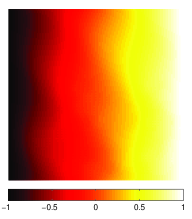
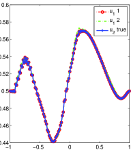
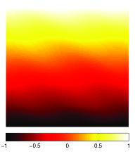
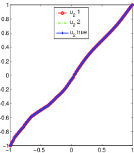
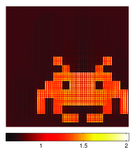
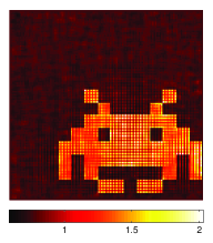
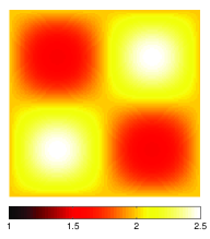
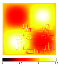
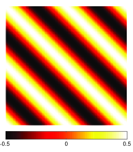
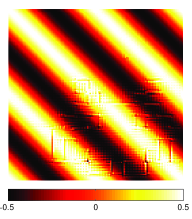
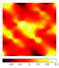
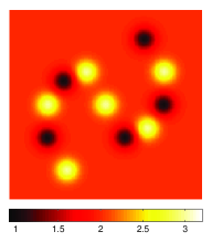
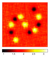
In the following examples, the conductivity tensor is described by the triplet of scalar functions such that with given in (36). Note that . The anisotropy coefficients in Fig. 11(a)&1(b) are used in all experiments, while the determinant may be either one of the two functions displayed in Figs. 11(c)&1(d).


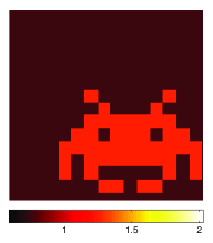
We sometimes perturb the internal functionals with random noise of the form
| (81) |
where is the noise level and random is a N+1N+1 matrix of random entries with uniform density over , to which we have applied a slight regularization by convolving it with the averaging filter ones(3)/9 (e.g. using the MatLab imfilter function).
Reconstruction of the anisotropy from noiseless data and solutions.
Let the two systems and be associated with and respectively, where are given by
We first compute the data by solving the three forward problems (3) and then computing over the grid. We then compute the vector fields and in the Gram-Schmidt case, where the transfer matrices such that for are given by
with and . and then admit the following expressions:
| (82) |
Once are generated numerically, we then reconstruct the functions that characterize via formulas (44).
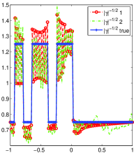
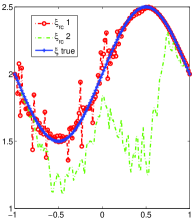
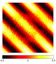
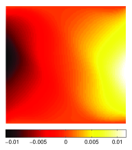
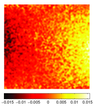
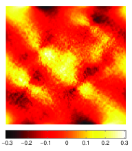
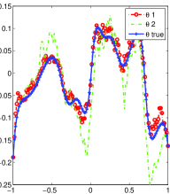
The simulation of that appears in (82) is presented for the smooth in the absence of noise on Fig. 33(a) and in the presence of one percent of noise on Fig. 33(b).
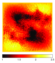
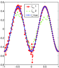
The reconstruction of is performed for both forms of in Figs.11(c)&1(d) and the results are presented in Fig.2. In the smooth case, the reconstructed cannot be distinguished visually from the exact coefficients and are thus not represented. Relative () errors for and are () and (), respectively. In the second case, the singularities of create artifacts on the reconstructions, see Fig. 22(b)&2(f), and the relative errors for and increase to () and (), respectively.

Reconstruction of the anisotropy from noisy data and solutions, .
Figs. 33(a)&3(b) show that even very small amounts of noise in the three available internal functionals significantly affect the reconstruction of the anisotropic coefficients. The presence of noise creates local extrema for the function so that its gradient and may vanish and (44) may no longer hold.
To address this lack of robustness, we increase the number of available internal functionals to for , which correspond to the boundary conditions . Instead of solving the linear system (43), we solve the normal equation (in the -minimizing sense) associated with the over-determined linear equations, each pair of which looks like (43) with for . The normal system reads
and thus may be inverted as
| (83) |
Results are shown after iterations in Fig. 2, where for , we used the following boundary conditions
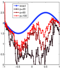
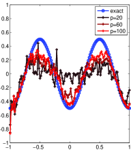
The relative errors for and are and , respectively. The effect of the number of measurements on the reconstruction can been on Fig. 3. We observe a very slow convergence, which is consistent with the central limit theory, as increases. The slow convergence may be considerably sped up by adding more constraining prior information on such as for instance regularity or sparsity constraints. We do not explore this aspect here.
Reconstruction of via .
We now assume that the anisotropy is known or reconstructed, and solve for by first applying the divergence operator to (52) and then for by applying the divergence operator to (61). For both Poisson equations, we use exact data as boundary conditions. In the Gram-Schmidt case, and the vector fields are given by (recall that )
where the data come from solutions with boundary conditions for .
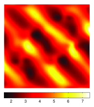
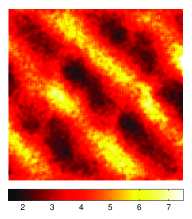

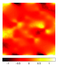
The isotropic part modeled by is given in Fig. 55(e). Fig. 4 displays the corresponding internal functionals with and without noise. Fig. 5 displays the reconstructed and . These reconstructions are quite robust to noise when the anisotropy is known: the relative () errors are () for and () for with noiseless data, and () for and () for with noise. If the anisotropy is first reconstructed from noisy data, this certainly has repercussions on the reconstructed , as can be seen in Fig. 55(c)&5(g). In this case, the () relative errors are () for and () for .

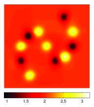
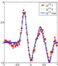
Reconstruction of via .
We still assume known with the coefficients displayed in Fig. 2. The boundary conditions are the same as in the preceding example. The isotropic component is now given in Fig. 66(e) and corresponds to a non-smooth coefficient. In this context, we first reconstruct by solving system (66), after which we reconstruct by taking the divergence of (73). The relative () errors are () for , () for and () for in the case of noisefree data, and () for , () for and () for in the case of data polluted with noise. See Fig. 6 for the display of some reconstructions. Based on the numerical simulations that we have performed, this reconstruction method and the previous one are very comparable in terms of accuracy and robustness.
7 Conclusions
This paper presented an explicit reconstruction procedure for a diffusion tensor from power density internal functionals for with .
Provided that four illuminations are selected so that the qualitative properties (11) and (12) of the corresponding solutions are verified, we obtained an explicit expression for the anisotropic part of and showed in Theorem 2.2 that errors in the uniform norm of the anisotropy were controlled by errors in the uniform norm of derivatives of the functionals .
Once the anisotropy is reconstructed, or is known by other means, we have presented two methods to reconstruct the determinant of . The first functional is based on first reconstructing the angle between and . The second method is based on solving a coupled system of elliptic equations for . In both cases, we need that the three internal functionals and satisfy (7) in . And in both cases, we obtain that the error in the uniform norm of the derivative of the determinant was controlled by errors in the uniform norm of derivatives of the functionals .
This shows that the reconstruction of the determinant of is more stable than that of the anisotropy of . Such a statement was verified by numerical simulations. In the presence of very limited noise generated by the numerical discretization, we obtained accurate reconstructions of the full tensor . However, even in the presence of quite small additional noise on the functionals , we observed that the reconstruction of the anisotropy was degrading very rapidly. On the other hand, the reconstruction of the determinant of , assuming the anisotropy known, proved very stable even in the presence of significant noise in the available functionals. In practice, this shows that appropriate regularization procedures on the anisotropy need to be introduced, for instance based on regularity or sparsity assumptions. This now standard step was not considered here.
The functionals emerging from ultrasound modulation experiments are thus sufficiently rich to provide unique reconstructions of arbitrary diffusion tensors. This should be contrasted with reconstruction procedures based on boundary measurements of elliptic solutions, in which diffusion tensors are defined up to an arbitrary change of variables inside the domain of interest [3]. Moreover, reconstructions are stable with a resolution that is essentially independent of the location of the point inside the domain of interest.
The reconstruction procedure presented here is two dimensional. Although this is not presented here, the reconstruction of the determinant of knowing its anisotropy generalizes to the -dimensional setting using techniques developed in [7, 16]. The reconstruction of the full diffusion tensor in dimension remains open at present.
Acknowledgment
This research was supported in part by National Science Foundation Grants DMS-0804696 and DMS-1108608. The authors would like to thank the referees for their valuable comments.
References
- [1] H. Ammari, E. Bonnetier, Y. Capdeboscq, M. Tanter and M. Fink, Electrical impedance tomography by elastic deformation, SIAM J. Appl. Math., 68(6), pp. 1557-1573.
- [2] K. Astala, T. Iwaniec and G. Martin, Elliptic Partial Differential Equations and Quasiconformal Mappings in the Plane, Princeton University Press (2009).
- [3] K. Astala, M. Lassas and L. Päivärinta, Calderón’s Inverse Problem for Anisotropic Conductivity in the Plane, Comm. in Partial Diff. Eq., 30; 207-224, 2005.
- [4] G. Alessandrini and V. Nesi, Univalent -harmonic mappings, Arch. Rat. Mech. Anal., 158:155-171, 201.
- [5] K. Astala and L. Päivärinta, Calderón’s inverse conductivity problem in the plane, Annals of Math., 163 (2006), pp. 165-299.
- [6] G. Bal, Hybrid inverse problems and internal functionals (review paper), to appear in Inside Out, 2012.
- [7] G. Bal, E. Bonnetier, F. Monard and F. Triki, Inverse diffusion from knowledge of power densities, to appear in Inverse Problems and Imaging, 2012. arXiv:1110.4577.
- [8] G. Bal and G. Uhlmann, Inverse diffusion theory for photoacoustics, Inverse Problems, 26(8) (2010), p. 085010.
- [9] A. Calderón, On an inverse boundary value problem, Seminar on Numerical Analysis and its Applications to Continuum Physics, Soc. Brasileira de Matematica, Rio de Janeiro, (1980), pp. 65–73.
- [10] Capdeboscq, Fehrenbach, de Gournay and Kavian, Imaging by Modification: Numerical Reconstruction of Local Conductivities from Corresponding Power Density Measurements, Siam Journal on Imaging Sciences, 2, pp. 1003-1030 (2009).
- [11] L.C. Evans, Partial Differential Equations, Graduate Studies in Mathematics, Vol. 19, AMS.
- [12] P. Kuchment and L. Kunyansky, Synthetic focusing in ultrasound modulated tomography, Inverse Problems and imaging, Volume 4, No. 4, 2010, pp. 665-673.
- [13] P. Kuchment and L. Kunyansky, 2D and 3D reconstructions in acousto-electric tomography, Inverse Problems 27, 2011, 055013.
- [14] P. Kuchment and D. Steinhauer, Stabilizing inverse problems by internal data, preprint, 2011. arXiv:1110.1819v2.
- [15] J.M. Lee, Riemannian Manifolds, An Introduction to Curvature, Springer.
- [16] F. Monard and G. Bal, Inverse diffusion problems with redundant internal information, to appear in Inverse Problems and Imaging, 2012. arXiv:1106.4277.
- [17] A. Nachman, A. Tamasan and A. Timonov, Reconstruction of planar conductivities in subdomains from incomplete data, SIAM J. Appl. Math. 70, pp. 3342–3362.
- [18] J. Sylvester and G. Uhlmann, A global uniqueness theorem for an inverse boundary value problem, Ann. of Math., 125(1) (1987), pp. 153–169.
