1 Introduction

In classical optics, the concepts of intensity and phase of optical fields have a well-defined meaning. The oscillating real electromagnetic field associated with single mode, $E=A\cos(\Phi)$, has a well-defined amplitude and phase. Apart from a constant factor, the squared real amplitude, $A^{2}$, is the intensity of the field. In classical electrodynamics, contrary to quantum electrodynamics, there is no real need to use complex numbers to describe the field. However, it is convenient to work with exponentials rather than cosine and sine functions, and complex amplitudes of the field, $E=A\exp(-{\rm i}\Phi)$, are commonly used to describe the field. The modulus squared of such an amplitude is the intensity of the field and the argument is the phase. Both the intensity and the phase can be measured simultaneously in classical optics. In quantum optics, it was quite natural to associate the photon number operator with the intensity of the field and somehow construct the phase operator conjugate to the number operator. The latter task, however, turned out not to be easy.

The first attempts to construct explicitly a quantum phase operator as a quantity conjugate to the number operator were made by [Dirac [1927]. His idea was to perform a polar decomposition of the annihilation operator, similar to the polar decomposition of the complex amplitude performed for classical fields. It turned out later that such a decomposition suffers from serious drawbacks, and the phase operator introduced in this way cannot be considered as a properly defined Hermitian phase operator. [Susskind and Glogower [1964] exposed the contradictions inherent in Dirac’s polar decomposition and introduced, instead of the phase operator that appeared to be non-Hermitian, the operators $\widehat{\cos}\Phi_{\rm SG}$ and $\widehat{\sin}\Phi_{\rm SG}$ corresponding to the cosine and sine of the phase. Unfortunately, these $\widehat{\cos}\Phi_{\rm SG}$ and $\widehat{\sin}\Phi_{\rm SG}$ operators, although being Hermitian, do not commute, so that they cannot represent a single phase angle. Historically, the idea to use $\widehat{\cos}\Phi$ and $\widehat{\sin}\Phi$ as Hermitian operators describing the phase, was first raised by [Louisell [1963] in his short Letter, but he did not construct the explicit form of these operators. [Carruthers and Nieto [1968], in their review paper, gave a detailed record of the problems encountered on the way to constructing of the Hermitian phase operator and discussed thoroughly the properties of $\widehat{\cos}\Phi_{\rm SG}$ and $\widehat{\sin}\Phi_{\rm SG}$ operators. From their analysis it became clear that it is the boundedness of the photon number spectrum which does not allow for negative values, and which precludes the existence of a properly defined Hermitian phase operator in the infinite-dimensional Hilbert space. The difficulty in finding the form of the Hermitian phase operator led to the widespread belief that no such operator exists, although there were a number of ingenious attempts to construct a suitable operator within the infinite-dimensional Hilbert space ([Garrison and Wong [1970, Turski [1972], [Popov and Yarunin [1973] [?, ?], [Paul [1974, Damaskinsky and Yarunin [1978], [Galindo [1984b] [?, ?]). It was known [Newton [1980, Barnett and Pegg [1986, Lukš and Peřinová [1991, Lukš, Peřinová and Křepelka [1992a] that extension of the oscillator energy spectrum to negative values allows for the mathematical construction of the Hermitian phase operator, but this solution was unsatisfactory because of its recourse to unphysical states.

Recently, [Pegg and Barnett [1988] [?, ?] (see also [Barnett and Pegg [1989] [?, ?, ?, ?], [Pegg, Barnett and Vaccaro [1989, Barnett, Pegg and Vaccaro [1990, Pegg, Vaccaro and Barnett [1990], [Vaccaro and Pegg [1990a], [?, ?, ?], [Vaccaro, Barnett and Pegg [1992]) have found a way out of the difficulties with construction of a Hermitian phase operator. The key idea in the development of the Hermitian optical phase operator was abandonment of the conventional infinite-dimensional Hilbert space for the description of quantum states of a single field mode. They introduced, instead, a state space ${\cal H}^{(\sigma)}$ of formally finite dimension together with a prescription for taking the infinite-dimensional limit only after c-number expectation values and moments have been calculated. This idea reintroduced a symmetry to the photon number spectrum, which became bounded not only from below but also from above, and removed the main obstacle in constructing a Hermitian phase operator. An essential and indispensable ingredient of the Pegg-Barnett construction is the way the infinite-dimensional limit is taken, which distinguishes it from the quantum-mechanical constructions based on finite-dimensional spaces that have been studied before ([Lévy-Leblond [1973] [?, ?, ?], [Santhanam and Tekumalla [1976], [Santhanam [1976] [?, ?, ?], [Santhanam and Sinha [1978, Goldhirsh [1980]), but in which, when the limiting procedure has been applied for the phase operator, the original problems reappeared. The consequences of the limiting procedure in the Pegg-Barnett approach have been discussed by [Barnett and Pegg [1992], and [Gantsog, Miranowicz and Tanaś [1992]. The proposal of the Pegg-Barnett approach has renewed interest in the problem of the proper description of the quantum-optical phase.

Almost at the same time, [Shapiro, Shepard and Wong [1989] (see also [Shapiro and Shepard [1991]) used an alternative approach based on the quantum estimation theory and probability operator measures [Helstrom [1976] to describe the phase properties of optical fields. This approach does not rely on the existence of the Hermitian phase operator but rather on the existence of the eigenstates of the Susskind-Glogower nonunitary exponential phase operator [Susskind and Glogower [1964]. The eigenstates of the Susskind-Glogower phase operators form a basis for the probability operator measures. The [Shapiro, Shepard and Wong [1989] idea has gained some popularity ([Hall [1991] [?], [Hall and Fuss [1991, Schleich, Dowling and Horowicz [1991, Braunstein, Lane and Caves [1992, Braunstein [1992], [Hradil [1992a] [?, ?], [Hradil and Shapiro [1992, Lane, Braunstein and Caves [1993, Jones [1993, Shapiro [1993]). It turned out, however, that it gives for physical states [i.e., states with a finite mean number of photons (finite energy and its higher moments)], the same results as the Pegg-Barnett approach after the limit transition to the infinite-dimensional space. The eigenkets of the Susskind-Glogower exponential phase operators can be used in a similar fashion as coherent states (eigenkets of the annihilation operator) to define the resolution of the system operators; e.g., the phase operator ([Lukš and Peřinová [1991] [?, ?], [Brif and Ben-Aryeh [1994a] [?, ?], [Vaccaro and Ben-Aryeh [1995]. In this case the ordering of the phase exponentials is relevant, and, if the antinormal ordering is taken, the results agree with those obtained from the Pegg-Barnett formalism.

Another way to describe the phase properties of the field is to use quasiprobability distribution functions. The idea behind this approach is relatively simple: to integrate the suitable quasiprobability distribution function, such as the Glauber-Sudarshan $P$-function, Wigner function, or Husimi $Q$-function over the “radial” variable and getting in this way a corresponding phase distribution, which can then be applied in calculations of the mean values of the phase-dependent quantities. Since the quasiprobability description of the quantum state of the system can be in some cases associated with realistic measurements performed on the system, this approach to the phase problem has focused the attention of many authors (see §2.2). The phase distribution functions obtained by integrating the quasidistributions are different for different quasidistributions, and they are all different from the Pegg-Barnett phase distribution. The situation is even worse because for some states of the field the $P$-function and the Wigner function take on negative values, and the corresponding phase distribution can also be negative. This means that such phase distributions must be used with some care, but in many cases this approach gives results describing properly the phase properties of the field.

[Noh, Fougères and Mandel [1991] [?, ?, ?, ?, ?, ?, ?, ?] (see also [Fougéres, Monken and Mandel [1994], [Barnett and Pegg [1993], [Hradil [1993a] [?, ?], [Hradil and Bajer [1993]) presented an operational approach to the quantum phase problem. Their idea is to define phase in terms of what actually is, or can be, measured. They do not search for a phase operator which would satisfy some mathematical criteria, but start their considerations from the experimental schemes usual in classical phase measurements. Examining various measuring schemes, they identify certain operators, $\hat{C}_{M}$ and $\hat{S}_{M}$, corresponding to the measured cosine and sine of the phase difference between two fields. As a result, [Noh, Fougères and Mandel [1991] came to the conclusion that there is no unique phase operator, and that different measuring schemes correspond to different operators. Nevertheless, recent theoretical studies [Riegler and Wódkiewicz [1994, Englert and Wódkiewicz [1995, Englert, Wódkiewicz and Riegler [1995] show that the intrinsic Hermitian phase operator associated with the [Noh, Fougères and Mandel [1991] apparatus can be found. The phase distribution measured in this experiment, under some conditions, is the radius-integrated Q-function ([Freyberger and Schleich [1993, Leonhardt and Paul [1993a], [Freyberger, Vogel and Schleich [1993a] [?, ?], [Bandilla [1993, Khan and Chaudhry [1994]). The measurements of [Noh, Fougères and Mandel [1991] are important since until then only isolated phase measurements were available performed by [Gerhardt, Büchler and Litfin [1974] ([Gerhardt, Welling and Frölich [1973], and for theoretical analysis see also [Nieto [1977, Lévy-Leblond [1977], [Lynch [1987] [?, ?, ?, ?], [Gerry and Urbanski [1990, Bandilla [1991, Tsui and Reid [1992], [Matthys and Jaynes [1980], [Walker and Carroll [1984] [?, ?]).

Quite recently, another experimental technique, optical homodyne tomography, was invented and applied to measurements of the quantum state of the field [Smithey, Faridani, and Raymer [1993, Beck, Smithey and Raymer [1993, Beck, Smithey, Cooper and Raymer [1993, Smithey, Beck, Cooper and Raymer [1993, Smithey, Beck, Cooper, Raymer and Faridani [1993] allowing quantum phase mean values to be calculated from the measured field density matrix. This technique opens new possibilities for quantum measurements. Overviews of various techniques for measuring phase distributions are presented by, e.g., [Leonhardt and Paul [1993b, Paul and Leonhardt [1994], [Peřina, Hradil and Jurčo [1994] and [Lynch [1995].

Another interesting approach to the phase problem was presented by [Bergou and Englert [1991]. They introduced the idea of phasors and phasor bases that can be used for studying possible candidates for the quantum phase operators. Different phasor bases lead to different phase operators, and according to [Bergou and Englert [1991] extrapolation of the classical concept of phase to the quantum regime is not unique.

Since the absolute phase of the single-mode field is not accessible for measurements, and it is always the difference with respect to a reference phase that we are forced to deal with in real measurements, it is tempting to define the phase-difference operator as a fundamental quantity describing the optical phase. [Luis and Sánchez-Soto [1993c] [?, ?] have defined a Hermitian phase-difference operator, which is in fact a polar decomposition of the Stokes operators for the two-mode field, and it is not the same as the difference of the two Pegg-Barnett operators. The difference between the two is most pronounced for weak fields. [Ban [1991a] [?, ?, ?, ?] has introduced yet another phase operator, based on the two-mode description of the field. In recent years, many different aspects of the quantum phase problem have been studied ([Barnett, Stenholm and Pegg [1989], [Nath and Kumar [1989] [?, ?, ?], [Chaichian and Ellinas [1990, Lakshmi and Swain [1990, Summy and Pegg [1990], [Hradil [1990] [?, ?], [Lukš and Peřinová [1990] [?, ?, ?, ?], [Vourdas [1990] [?, ?, ?], [Adam, Janszky and Vinogradov [1991, Cibils, Cuche, Marvulle and Wreszinski [1991, Dowling [1991], [Ellinas [1991a] [?, ?, ?], [Gantsog and Tanaś [1991d, Nath and Kumar [1991a], [Orszag and Saavedra [1991a] [?, ?], [Paul [1991, Tanaś [1991, Wilson-Gordon, Bužek and Knight [1991, Agarwal, Chaturvedi, Tara and Srinivasan [1992, Bandilla [1992, Janszky, Adam, Bertolotti and Sibilia [1992], [Lukš, Peřinová and Křepelka [1992b] [?, ?], [Ritze [1992, Smith, Dubin and Hennings [1992, Tsui and Reid [1992] [Agarwal [1993, Agarwal, Scully and Walther [1993, Ban [1993, Białynicki-Birula, Freyberger and Schleich [1993, Chizhov, Gantsog and Murzakhmetov [1993, Chizhov and Murzakhmetov [1993, Daeubler, Miller, Risken and Schoendorff [1993], [d’Ariano and Paris [1993] [?, ?], [Jex and Drobný [1993, Luis and Sánchez-Soto [1993a, Stenholm [1993, Schieve and McGowan [1993, Tu and Gong [1993, Agarwal, Graf, Orszag, Scully and Walther [1994, Belavkin and Bendjaballah [1994], [Vaccaro and Pegg [1994a] [?, ?, ?], [Białynicka-Birula and Białynicki-Birula [1994] [?, ?], [Das [1994, Franson [1994, Gennaro, Leonardi, Lillo, Vaglica and Vetri [1994, Opatrný [1994, Sánchez-Soto and Luis [1994, Schaufler, Freyberger and Schleich [1994]), and the number of publications on the subject is growing steadily. Various conceptions of the quantum-optical phase have been described by [Barnett and Dalton [1993] in a special issue of Physica Scripta devoted to “Quantum phase and phase dependent measurements”, and in the same issue one can find very interesting historical facts, given by [Nieto [1993], concerning the development of our knowledge on quantum phase.

Nowadays, although the quantum phase is still a subject of some controversy, significant progress has been achieved in clarifying the status of the quantum-mechanical phase operator, describing the phase properties of optical fields in terms of various phase distribution functions, and measuring phase-dependent physical quantities. We can now risk the statement that, despite the existence of various different conceptions of phase, we are en route to unified view and understanding of the quantum-optical phase.

It is not our aim in this review article to give a detailed account of different descriptions of the quantum phase showing their similarities and differences. We will not focus our attention on the quantum phase formalisms, which are interesting on their own right and deserve separate treatment. We shall instead concentrate on the description of the quantum properties of real-field states which are generated in various nonlinear optical processes. Nonlinear optical phenomena are sources of optical fields, the statistical properties of which have been changed in a nontrivial way as a result of nonlinear transformation. Quantum phase properties are among those statistical properties which undergo nonlinear changes, and fields generated in different nonlinear processes have different phase properties. With the existing phase formalisms, the quantum-phase properties of such fields can be studied in a systematic way, and quantitative comparisons between different quantum-field states can be made. Using the Pegg-Barnett phase formalism and the phase formalism based on the $s$-parametrized quasidistribution functions, we will study a number of both one- and two-mode field states from the point of view of their phase properties.

2 Phase formalisms

At the very beginning of quantum electrodynamics, [Dirac [1927] raised the idea that the optical phase should be described by a Hermitian phase operator canonically conjugate to the number operator; that is, for the single-mode field the two operators should obey the canonical commutation relation

$$[\hat{\Phi},\hat{n}] = -{\rm i}.$$ (2.1)

This commutation relation implies directly the “traditional” Heisenberg uncertainty relation

$${\langle(\Delta{\hat{n}})^{2}\rangle}{\langle(\Delta{\hat{\Phi}})^{2}\rangle}\geq{1\over 4},$$ (2.2)

which appeared to be wrong [Susskind and Glogower [1964, Carruthers and Nieto [1968]. Closer investigation of the commutator (2.1) showed that the matrix elements of the phase operator $\hat{\Phi}$ in a number-state basis are undefined [Louisell [1963]:

$$(n-n^{{}^{\prime}}){\langle n^{{}^{\prime}}|\,}\hat{\Phi}{\,|n\rangle}\;=\;-{\rm i}\delta_{nn^{{}^{\prime}}}.$$ (2.3)

Since it was suggested that the problems in eq. (2.3) are due to the multivalued nature of $\hat{\Phi}$, [Louisell [1963] introduced the operators $\widehat{\cos}\Phi$ and $\widehat{\sin}\Phi$, which should, as he suggested, satisfy the commutation relations:

$$\left[\widehat{\cos}\Phi,\hat{n}\right] = {\rm i}\widehat{\sin}\Phi,$$

$$\left[\widehat{\sin}\Phi,\hat{n}\right] = -{\rm i}\widehat{\cos}\Phi.$$ (2.4)

However, [Louisell [1963] did not give the explicit form of the cosine and sine operators; thus, his idea did not help much in solving the phase problem. Moreover, it turned out that the problem expressed in eq. (2.3) was not due to the multivalued nature of $\hat{\Phi}$, but rather to the improper application of the correspondence between the Poisson bracket and the commutator. [Susskind and Glogower [1964] returned to the original Dirac idea of polar decomposition of the creation and annihilation operators and introduced the exponential phase operators:

$$\widehat{\exp}({\rm i}\Phi_{\rm SG}) \equiv \sum_{n=0}^{\infty}|n\rangle\langle n+1|,$$ (2.5)

$$\widehat{\exp}(-{\rm i}\Phi_{\rm SG}) \equiv \bigr{[}\widehat{\exp}({\rm i}\Phi_{\rm SG})\bigl{]}^{\dagger}.$$ (2.6)

From eqs. (2.5) and (2.6) one obtains:

$$\widehat{\exp}({\rm i}\Phi_{\rm SG})\widehat{\exp}(-{\rm i}\Phi_{\rm SG}) = 1,$$

$$\widehat{\exp}(-{\rm i}\Phi_{\rm SG})\widehat{\exp}({\rm i}\Phi_{\rm SG}) = 1-|0\rangle\langle 0|,$$ (2.7)

which explicitly shows the non-unitarity of the Susskind-Glogower phase operator.

The Susskind-Glogower exponential operators (2.5) and (2.6) allow for constructing two Hermitian combinations corresponding to cosine and sine of the phase. However, the two combinations do not commute, so they cannot be considered as describing a single phase angle. Despite this deficiency, the Susskind-Glogower phase operators were widely used in description of optical fields until recently. The eigenkets of the Susskind-Glogower operator (2.5), given by

$${\,|\theta\rangle} \equiv \frac{1}{\sqrt{2\pi}}\sum_{n=0}^{\infty}\exp({\rm i}n\theta){\,|n\rangle},$$ (2.8)

generate the resolution of the identity, and, despite their nonorthogonality, they can be used to form the probability operator measure applied to the phase description by [Shapiro and Shepard [1991].

[Garrison and Wong [1970] made an attempt to construct a Hermitian phase operator in the infinite-dimensional Hilbert space which, as they demanded, should satisfy the canonical commutation relation (2.1). Their work was almost completely forgotten. [Bergou and Englert [1991] have made a comparison of the Garrison-Wong and Pegg-Barnett phase operators, pointing out that if the limit to infinite-dimensional space is performed on the latter operator (but not on the expectation values), the former operator is obtained. In their view the Pegg-Barnett phase formalism is only an approximation to the “correct” phase formalism. [Bergou and Englert [1991] introduced their own quantum-phase description, which has not gained broader acceptance. Nevertheless, their paper is an essential contribution which clarifies a number of points in the quantum-phase problem. The Garrison-Wong approach turned out to lead to phase distributions which are asymmetric and difficult to accept on physical grounds [Gantsog, Miranowicz and Tanaś [1992]; e.g., even the vacuum is phase-anisotropic. For reference, we give a sketch of their approach in Appendix A.

The renewed interest in quantum-phase problems has resulted in a reexamination of some of the earlier approaches and the creation of other, completely new descriptions. From a number of different phase formalisms that are now available, we choose only two, which we shall apply for the description of the phase properties of fields generated in various nonlinear optical processes. These are: the Pegg-Barnett phase formalism, which represents the canonical phase formalism based on the idea of finding a Hermitian phase operator, and another formalism based on the description of the optical phase through $s$-parametrized phase distributions, which for some values of $s$ represents the experimentally measured phase probability distributions.

2.1 Pegg-Barnett phase formalism

[Pegg and Barnett [1988] [?, ?] (and [Barnett and Pegg [1989]) introduced the Hermitian phase formalism, which is based on the observation that, in a finite-dimensional state space, the states with well-defined phase exist [Loudon [1973]. Thus, they restrict the state space to a finite $(\sigma+1)$-dimensional Hilbert space ${\cal H}^{(\sigma)}$ spanned by the number states $|0\rangle$, $|1\rangle$,…, $|\sigma\rangle$. In this space they define a complete orthonormal set of phase states by:

$$|\theta_{m}\rangle = \frac{1}{\sqrt{\sigma+1}}\>\sum_{n=0}^{\sigma}\exp({\rm i}n\theta_{m})\,|n\rangle,\hskip 28.45274ptm=0,1,\ldots,\sigma\,,$$ (2.9)

where the values of $\theta_{m}$ are given by

$$\theta_{m} = \theta_{0}+\frac{2\pi m}{\sigma+1}.$$ (2.10)

The value of $\theta_{0}$ is arbitrary and defines a particular basis set of ($\sigma+1$) mutually orthogonal phase states. The number state $|n\rangle$ can be expanded in terms of the $|\theta_{m}\rangle$ phase state basis as

$$|n\rangle = \sum_{m=0}^{\sigma}|\theta_{m}\rangle\langle\theta_{m}|n\rangle\;=\;\frac{1}{\sqrt{\sigma+1}}\sum_{m=0}^{\sigma}\exp(-{\rm i}n\theta_{m})|\theta_{m}\rangle.$$ (2.11)

From eqs. (2.9) and (2.11) we see that a system in a number state is equally likely to be found in any state $|\theta_{m}\rangle$, and a system in a phase state is equally likely to be found in any number state $|n\rangle$.

The Pegg-Barnett (PB) Hermitian phase operator is defined as

$${\hat{\Phi}_{\theta}}\>\equiv\>\left(\hat{\Phi}_{\theta_{0}}^{(\sigma)}\right)_{\rm PB} = \sum_{m=0}^{\sigma}\theta_{m}\,|\theta_{m}\rangle\langle\theta_{m}|.$$ (2.12)

Of course, the phase states (2.9) are eigenstates of the phase operator (2.12) with the eigenvalues $\theta_{m}$ restricted to lie within a phase window between $\theta_{0}$ and $\theta_{0}+2\pi\sigma/(\sigma+1)$. The Pegg-Barnett prescription is to evaluate any observable of interest in the finite basis (2.9), and only after that to take the limit $\sigma\rightarrow\infty$.

Since the phase states (2.9) are orthonormal, $\langle\theta_{m}|\theta_{m^{\prime}}\rangle=\delta_{mm^{\prime}}$, the $k$th power of the Pegg-Barnett phase operator (2.12) can be written as

$${\hat{\Phi}_{\theta}}^{k} = \sum_{m=0}^{\sigma}\theta_{m}^{k}\,|\theta_{m}\rangle\langle\theta_{m}|.$$ (2.13)

Substituting eqs. (2.9) and (2.10) into eq. (2.12) and performing summation over $m$ yields explicitly the phase operator in the Fock basis:

$${\hat{\Phi}_{\theta}} = \theta_{0}\>+\>\frac{\sigma\pi}{\sigma+1}\>+\>\frac{2\pi}{\sigma+1}\sum_{n\neq n^{\prime}}\frac{\exp[{\rm i}\,(n-n^{\prime})\theta_{0}]\,|n\rangle\langle n^{\prime}|}{\exp[{\rm i}\,(n-n^{\prime})2\pi/(\sigma+1)]-1}\>.$$ (2.14)

It is readily apparent that the Hermitian phase operator ${\hat{\Phi}_{\theta}}$ has well-defined matrix elements in the number-state basis and does not suffer from such problems as the original Dirac phase operator. A detailed analysis of the properties of the Hermitian phase operator was given by [Pegg and Barnett [1989] and [Barnett and Pegg [1989].

The unitary phase operator $\exp({\rm i}{\hat{\Phi}_{\theta}})$ can be defined as the exponential function of the Hermitian operator ${\hat{\Phi}_{\theta}}$. This operator acting on the eigenstate $|\theta_{m}\rangle$ gives the eigenvalue $\exp({\rm i}\theta_{m})$, and can be written as ([Pegg and Barnett [1988] [?, ?]):

$$\exp({\rm i}{\hat{\Phi}_{\theta}}) \equiv \sum_{n=0}^{\sigma-1}|n\rangle\langle n+1|+\exp\bigl{[}{\rm i}(\sigma+1)\theta_{0}\bigr{]}|\sigma\rangle\langle 0|,$$ (2.15)

Its Hermitian conjugate is

$$[\exp({\rm i}{\hat{\Phi}_{\theta}})]^{\dagger}=\exp(-{\rm i}{\hat{\Phi}_{\theta}})$$ (2.16)

with the same set of eigenstates $|\theta_{m}\rangle$ but with eigenvalues $\exp(-{\rm i}\theta_{m})$. This is the last term in eq. (2.15) that distinguishes the unitary phase operator from the Susskind-Glogower phase operator [Susskind and Glogower [1964]. The first sum in eq. (2.15) reproduces the Susskind-Glogower phase operator if the limit $\sigma\rightarrow\infty$ is taken. In contrast to the Pegg-Barnett unitary phase operator, the Susskind-Glogower exponential operator (2.5) is defined as a whole and is not unitary, as is apparent from eq. (2.7). The sine and cosine operators in the Pegg-Barnett formalism are the sine and cosine functions of the Hermitian phase operator ${\hat{\Phi}_{\theta}}$. They are more consistent with the classical notion of phase than their counterparts in the Susskind-Glogower phase formalism. In particular, they satisfy the “natural” relations:

$$\cos^{2}{\hat{\Phi}_{\theta}}+\sin^{2}{\hat{\Phi}_{\theta}} = 1,$$ (2.17)

$$\bigl{[}\cos{\hat{\Phi}_{\theta}},\sin{\hat{\Phi}_{\theta}}\bigr{]} = 0,$$ (2.18)

$$\langle n|\cos^{2}{\hat{\Phi}_{\theta}}|n\rangle=\langle n|\sin^{2}{\hat{\Phi}_{\theta}}|n\rangle = {1\over 2}.$$ (2.19)

The last relation is also true for the vacuum state, in sharp contrast to the Susskind-Glogower phase operators. This is consistent with the phase of vacuum being random, as well as for any other number state.

The Pegg-Barnett phase operator (2.14), expressed in the Fock basis, readily gives the phase-number commutator [Pegg and Barnett [1989]:

$$[{\hat{\Phi}_{\theta}},\hat{n}] = -\frac{2\pi}{\sigma+1}\sum_{n\neq n^{\prime}}\frac{(n-n^{\prime})\exp[{\rm i}(n-n^{\prime})\theta_{0}]}{\exp[{\rm i}(n-n^{\prime})2\pi/(\sigma+1)]-1}|n\rangle\langle n^{\prime}|.$$ (2.20)

Equation (2.20) looks very different from the famous Dirac postulate of the phase-number commutator (2.1). [Santhanam [1976] and [Pegg, Vaccaro and Barnett [1990] examined canonically conjugate operators in the finite-dimensional Hilbert space. According to the generalized definition by [Pegg, Vaccaro and Barnett [1990], the photon number and phase are indeed canonically conjugate variables, similar to momentum and position or angular momentum and azimuthal phase angle.

As the Hermitian phase operator is defined, one can calculate the expectation value and variance of this operator for a given state of the field $|f\rangle$. Moreover, the Pegg-Barnett phase formalism allows the introduction of the continuous-phase probability distribution which is a representation of the quantum state of the field and describes the phase properties of the field in a very spectacular fashion. Examples of such phase distributions for particular states of the field will be given later.

A general pure state of the field mode with a decomposition

$$|{f}\rangle=\sum_{n=0}^{\sigma}c_{n}|n\rangle,$$ (2.21)

can be re-expressed in the phase state basis, according to eq. (2.11), as

$$|{f}\rangle={1\over{\sqrt{\sigma+1}}}\sum_{n}\sum_{m}c_{n}\exp(-{\rm i}n\theta_{m})|\theta_{m}\rangle.$$ (2.22)

We should remark here that the coefficients $c_{n}$ in the decomposition (2.21) in a finite-dimensional space should differ from the coefficients in the infinite-dimensional space if the state ${\,|f\rangle}$ is to be normalized. A short discussion of this problem is given in Appendix B.

The phase probability distribution is given by [Pegg and Barnett [1989]:

$$\big{|}\langle\theta_{m}|{f}\rangle\big{|}^{2} = {1\over{\sigma+1}}{\left|\sum_{n}c_{n}\exp(-{\rm i}n\theta_{m})\right|}^{2},$$ (2.23)

which leads to the expectation value and variance of the phase operator:

$$\langle{f}|{\hat{\Phi}_{\theta}}|{f}\rangle = \sum_{m}\theta_{m}\big{|}\langle\theta_{m}|{f}\rangle\big{|}^{2},$$ (2.24)

$${\langle(\Delta{{\hat{\Phi}_{\theta}}})^{2}\rangle} = \sum_{m}(\theta_{m}-\langle{\hat{\Phi}_{\theta}}\rangle)^{2}\big{|}\langle\theta_{m}|{f}\rangle\big{|}^{2}.$$ (2.25)

If the field state $|{f}\rangle$ is a partial phase state, i.e., if the amplitude has the form

$$c_{n}=b_{n}\mbox{e}^{{\rm i}n\varphi},$$ (2.26)

the phase probability distribution (2.23) becomes

$$\big{|}\langle\theta_{m}|{f}\rangle\big{|}^{2} = {1\over{\sigma+1}}{\left|\sum_{n}b_{n}\exp[{\rm i}n(\varphi-\theta_{m})]\right|}^{2}$$ (2.27)

$$= {1\over{\sigma+1}}+{2\over{\sigma+1}}\sum_{n>k}b_{n}b_{k}\cos{\left[(n-k)(\varphi-\theta_{m})\right]}.$$

The mean and variance of ${\hat{\Phi}_{\theta}}$ will depend on the chosen value of $\theta_{0}$. [Judge [1964], in his description of the uncertainty relation for angle variables, suggested that the choice of phase window which minimizes the variance can be used to specify uniquely the mean or variance. For the partial phase state, the most convenient and physically transparent way of choosing $\theta_{0}$ is to symmetrize the phase window with respect to the phase $\varphi$. This means the choice

$$\theta_{0}=\varphi-{{\pi\sigma}\over{\sigma+1}},$$ (2.28)

and after introducing a new phase label

$$\mu=m-{\sigma\over 2},$$ (2.29)

the phase probability distribution (2.27) becomes

$$\big{|}\langle\theta_{\mu}|{f}\rangle\big{|}^{2} = {1\over{\sigma+1}}+{2\over{\sigma+1}}\sum_{n>k}b_{n}b_{k}\cos{\left[(n-k){{2\pi\mu}\over{\sigma+1}}\right]}$$ (2.30)

with $\mu$, which goes in integer steps from $-\sigma/2$ to $\sigma/2$. Since the distribution (2.30) is symmetrical in $\mu$, we immediately get, according to eqs. (2.28)–(2.30):

$$\langle{f}|{\hat{\Phi}_{\theta}}|{f}\rangle=\varphi.$$ (2.31)

This result means that for a partial phase state with phase $\varphi$, the choice of $\theta_{0}$ as in eq. (2.28) relates directly the expectation value of the phase operator with the phase $\varphi$. With this choice of $\theta_{0}$ the variance of the phase operator has a particularly simple form:

$${\langle(\Delta{{\hat{\Phi}_{\theta}}})^{2}\rangle} = {{4\pi^{2}}\over{(\sigma+1)^{2}}}\sum_{\mu=-\sigma/2}^{\sigma/2}\mu^{2}\big{|}\langle\theta_{\mu}|{f}\rangle\big{|}^{2}.$$ (2.32)

So-called physical states play a significant role in the Pegg-Barnett formalism. Physical states $|p\rangle$ are defined by [Pegg and Barnett [1989] as the states of finite energy. Most of the expressions in the Pegg-Barnett formalism take a much simpler form for physical states. For example, the commutator (2.20) reduces to

$$[{\hat{\Phi}_{\theta}},\hat{n}]_{p} = -{\rm i}\;[1-(\sigma+1)|\theta_{0}\rangle\langle\theta_{0}|],$$ (2.33)

a form more similar to the standard canonical commutation relation (2.1). On the other hand, when physical states are considered, we can simplify the calculation of the sum in eqs. (2.24) and (2.25) by replacing it by the integral in the limit as $\sigma$ tends to infinity. Since the density of states is $(\sigma+1)/2\pi$, we can write the expectation value of the $k$th power of the phase operator as

$$\langle f|{\hat{\Phi}_{\theta}}^{k}|f\rangle = \int\limits_{\theta_{0}}^{\theta_{0}+2\pi}{\rm d}\theta\,\theta^{k}{P(\theta)},$$ (2.34)

where the continuous-phase distribution ${P(\theta)}$ is introduced by

$$P(\theta)\;\equiv\;P_{\rm PB}(\theta) = \lim_{\sigma\rightarrow\infty}\frac{\sigma+1}{2\pi}|\langle\theta_{m}|f\rangle|^{2},$$ (2.35)

and $\theta_{m}$ has been replaced by the continuous-phase variable $\theta$. If the state $|f\rangle$ has the number-state decomposition (2.21), then the Pegg-Barnett phase distribution is  [Pegg and Barnett [1989]:

$${P(\theta)} = \frac{1}{2\pi}\left\{1+2{\rm Re}\sum_{n,m\atop m>n}c_{m}c_{n}^{*}\exp[-{\rm i}(m-n)\theta]\right\}.$$ (2.36)

In the case of fields being in mixed states described by the density matrix $\hat{\rho}$, formula (2.36) generalizes to

$${P(\theta)} = \frac{1}{2\pi}\left\{1+2{\rm Re}\sum_{m>n}\rho_{mn}\exp[-{\rm i}(m-n)\theta]\right\},$$ (2.37)

where $\rho_{mn}=\langle m|\hat{\rho}|n\rangle$ are the density matrix elements in the number-state basis. Equations (2.36) or (2.37) can be used for calculations of the Pegg-Barnett phase distribution for any state with known amplitudes $c_{n}$ or matrix elements $\rho_{mn}$. Despite the fact that they are exact, they can rarely be summed up into a closed form, and usually numerical summation must be performed to find the phase distribution. Such numerical summations have been widely applied in studying the phase properties of optical fields. The Pegg-Barnett phase distribution, eqs. (2.36) or (2.37), is obviously $2\pi$-periodic, and for all states with the density matrix diagonal in the number states, the phase distribution is uniform over the $2\pi$-wide phase window. These are nondiagonal elements of the density matrix that lead to the structure of the phase distribution. The Pegg-Barnett distribution is positive definite and normalized.

After introducing the continuous-phase distribution ${P(\theta)}$, formula (2.32) for the phase variance, if the symmetrization is performed, can be rewritten into the form:

$${\langle(\Delta{{\hat{\Phi}_{\theta}}})^{2}\rangle} = \int\limits_{-\pi}^{\pi}\theta^{2}{P(\theta)}\,{\rm d}\theta.$$ (2.38)

This means that as the phase distribution function ${P(\theta)}$ is known, all quantum-mechanical phase characteristics can be calculated with this function in a classical-like manner. The result for the variance (2.38) is [Barnett and Pegg [1989]:

$${\langle(\Delta{{\hat{\Phi}_{\theta}}})^{2}\rangle}={{\pi^{2}}\over 3}+4\sum_{n>k}b_{n}b_{k}{{(-1)^{n-k}}\over{(n-k)^{2}}}.$$ (2.39)

The value $\pi^{2}/3$ is the variance for the uniformly distributed phase, as in the case of a single number state.

For physical states there are some additional useful relations between the expectation values of the Pegg-Barnett phase operators and of the Susskind-Glogower phase operators. For example, the following relations hold [Vaccaro and Pegg [1989]:

$$\langle\exp({\rm i}m{\hat{\Phi}_{\theta}})\rangle_{p} = \langle\widehat{\exp}({\rm i}m\Phi_{\rm SG})\rangle_{p},$$ (2.40)

$$\langle\cos{\hat{\Phi}_{\theta}}\rangle_{p} = \langle\widehat{\cos}\Phi_{\rm SG}\rangle_{p},$$ (2.41)

$$\langle\sin{\hat{\Phi}_{\theta}}\rangle_{p} = \langle\widehat{\sin}\Phi_{\rm SG}\rangle_{p},$$ (2.42)

$$\langle\cos^{2}{\hat{\Phi}_{\theta}}\rangle_{p} = \langle\widehat{\cos}^{2}\Phi_{\rm SG}\rangle_{p}+{1\over 4}\langle(|0\rangle\langle 0|)\rangle_{p},$$ (2.43)

$$\langle\sin^{2}{\hat{\Phi}_{\theta}}\rangle_{p} = \langle\widehat{\sin}^{2}\Phi_{\rm SG}\rangle_{p}+{1\over 4}\langle(|0\rangle\langle 0|)\rangle_{p}.$$ (2.44)

where the subscript $p$ refers to a physical state expectation value.

2.2 Phase distributions from $s$-parametrized quasidistributions

According to [Cahill and Glauber [1969a] [?, ?], the $s$-parametrized quasidistribution function ${\cal W}^{(s)}(\alpha)$ describing a field state, can be derived from the formula

$${\cal W}^{(s)}(\alpha) = \frac{1}{\pi}\,{\rm Tr}\,\{\hat{\rho}\,\hat{T}{{}^{(s)}}(\alpha)\},$$ (2.45)

where the operator $\hat{T}{{}^{(s)}}(\alpha)$ is given by

$$\hat{T}{{}^{(s)}}(\alpha) = \frac{1}{\pi}\int\exp(\alpha\xi^{*}-\alpha^{*}\xi)\hat{D}{{}^{(s)}}(\xi)\,{\rm d}^{2}\xi,$$ (2.46)

$$\hat{D}{{}^{(s)}}(\xi) = {\rm e}^{s|\xi|^{2}/2}\hat{D}(\xi)$$ (2.47)

with $\hat{D}(\xi)$ being the displacement operator; $\hat{\rho}$ is the density matrix of the field, and we have introduced the extra $1/\pi$ factor with respect to the original definition of [Cahill and Glauber [1969b]. The operator $\hat{T}{{}^{(s)}}(\alpha)$ can be rewritten in the form [Cahill and Glauber [1969a]:

$$\hat{T}{{}^{(s)}}(\alpha) = \frac{2}{1-s}\sum_{n=0}^{\infty}\hat{D}(\alpha)|n\rangle\left(\frac{s+1}{s-1}\right)^{n}\langle n|\hat{D}^{\dagger}(\alpha),$$ (2.48)

which gives explicitly its $s$-dependence. So, the $s$-parametrized quasidistribution function ${\cal W}^{(s)}(\alpha)$ has the following form in the number-state basis:

$${\cal W}^{(s)}(\alpha) = \frac{1}{\pi}\sum_{m,n}\rho_{mn}\langle n|\hat{T}{{}^{(s)}}(\alpha)|m\rangle,$$ (2.49)

where the matrix elements of the operator (2.46) are given by [Cahill and Glauber [1969a]:

$$\langle n|\hat{T}^{(s)}(\alpha)|m\rangle = \left(\frac{n!}{m!}\right)^{1/2}\left(\frac{2}{1-s}\right)^{m-n+1}\left(\frac{s+1}{s-1}\right)^{n}$$ (2.50)

$$\times\;{\rm e}^{-{\rm i}(m-n)\theta}|\alpha|^{m-n}\exp\left(-\frac{2|\alpha|^{2}}{1-s}\right)L_{n}^{m-n}\left(\frac{4|\alpha|^{2}}{1-s^{2}}\right),$$

in terms of the associate Laguerre polynomials $L_{n}^{m-n}(x)$. In eq. (2.50) we have also separated explicitly the phase of the complex number $\alpha$ by writing

$$\alpha = |\alpha|{\rm e}^{{\rm i}\theta}.$$ (2.51)

In the following, the phase $\theta$ will be treated as the quantity representing the field phase.

With the quasiprobability distributions ${\cal W}^{(s)}(\alpha)$ the expectation values of the $s$-ordered products of the creation and annihilation operators can be obtained by proper integrations in the complex $\alpha$ plane. In particular, for $s=1,0,-1$, the $s$-ordered products are normal, symmetrical, and antinormal ordered products of the creation and annihilation operators, and the corresponding quasiprobability distributions are the Glauber-Sudarshan $P$-function, Wigner function, and Husimi $Q$-function.

By virtue of the relation inverse to eq. (2.49), given by [Cahill and Glauber [1969b]:

$$\hat{\rho} = \int{\rm d}^{2}\alpha\>\hat{T}^{(-s)}(\alpha)W{{}^{(s)}}(\alpha),$$ (2.52)

the Pegg-Barnett phase distribution (2.37) can be related to the $s$-parametrized quasidistribution function (2.45) as follows [Eiselt and Risken [1991]:

$$P(\theta) = \int{\rm d}^{2}\alpha\>K{{}^{(s)}}(\alpha,\theta)W{{}^{(s)}}(\alpha),$$ (2.53)

where the kernel is given by

$$K{{}^{(s)}}(\alpha,\theta) = \frac{1}{2\pi}\sum_{m,n}\langle n|\hat{T}^{(-s)}(\alpha)|m\rangle\exp[{\rm i}(m-n)\theta]$$ (2.54)

in terms of the matrix elements (2.50) for $(-s)$. The kernel (2.54) is convergent for $s>-1$ only. Nevertheless, the remaining relation between the Husimi $Q$-function and the Pegg-Barnett distribution can also be expressed by eq. (2.53), albeit with the following kernel [Miranowicz [1994]:

$$K^{(-1)}(\alpha,\theta) = \frac{1}{2\pi}\sum_{n,m}\int{\rm d}^{2}\beta\>\frac{(\alpha+\beta)^{m}(\alpha^{*}-\beta^{*})^{n}}{\sqrt{n!m!}}$$ (2.55)

$$\times\;\exp[{\rm i}(n-m)\theta-|\alpha|^{2}+\alpha\beta^{*}-\alpha^{*}\beta].$$

On integrating the quasiprobability distribution ${\cal W}^{(s)}(\alpha)$ over the “radial” variable $|\alpha|$, we get the “phase distribution” associated with this quasiprobability distribution. The $s$-parametrized phase distribution is thus given by

$${P^{(s)}(\theta)} = \int\limits_{0}^{\infty}{\cal W}^{(s)}(\alpha)|\alpha|\>{\rm d}|\alpha|$$ (2.56)

or equivalently by

$${P^{(s)}(\theta)} = \frac{1}{2}\int\limits_{0}^{\infty}{\cal W}^{(s)}(W,\theta)\>{\rm d}W,$$ (2.57)

where integration is performed over the intensity $W=|\alpha|^{2}$. Inserting eq. (2.49) into eq. (2.56) yields

$${P^{(s)}(\theta)} = \frac{1}{\pi}\sum_{m,n}\rho_{mn}\left(\frac{n!}{m!}\right)^{1/2}\left(\frac{2}{1-s}\right)^{m-n+1}\left(\frac{s+1}{s-1}\right)^{n}{\rm e}^{-{\rm i}(m-n)\theta}$$ (2.58)

$$\times\;\int\limits_{0}^{\infty}|\alpha|^{m-n}\exp\left(-\frac{2|\alpha|^{2}}{1-s}\right)L_{n}^{m-n}\left(\frac{4|\alpha|^{2}}{1-s^{2}}\right)|\alpha|\>{\rm d}|\alpha|.$$

If the definition of the Laguerre polynomial is invoked, the integrations in eq. (2.58) can be performed explicitly, and we get for the $s$-parametrized phase distribution a formula similar to the Pegg-Barnett phase distribution (2.37), which reads

$${P^{(s)}(\theta)} = \frac{1}{2\pi}\left\{1+2{\rm Re}\sum_{m>n}\rho_{mn}{\rm e}^{-{\rm i}(m-n)\theta}G^{(s)}(m,n)\right\}.$$ (2.59)

The difference between eqs. (2.37) and (2.59) lies in the coefficients $G^{(s)}(m,n)$, which are given by

$$G^{(s)}(m,n) = \left(\frac{2}{1-s}\right)^{\frac{m+n}{2}}\>\sum_{l=0}^{{\rm min}(m,n)}(-1)^{l}\left(\frac{1+s}{2}\right)^{l}$$ (2.60)

$$\times\;\sqrt{\left(n\atop l\right)\left(m\atop l\right)}\frac{\Gamma\left(\frac{m+n}{2}-l+1\right)}{\sqrt{(m-l)!(n-l)!}}.$$

The $s$-parametrized coefficients $G^{(s)}(m,n)$, [eq. (2.60)], can be rewritten in a compact form [Miranowicz [1994, Leonhardt, Vaccaro, Böhmer and Paul [1995] ($m\geq n$):

$$G^{(s)}(m,n) = \sqrt{\frac{n!}{m!}}\left(\frac{s+1}{s-1}\right)^{n}\left(\frac{2}{1-s}\right)^{(m-n)/2}$$ (2.61)

$$\times\;\;\Gamma\left(\frac{m-n}{2}+1\right)P_{n}^{\left(m-n,-\frac{1}{2}(m+n)\right)}\left(\frac{s-3}{s+1}\right)$$

in terms of the Jacobi polynomials $P_{n}^{(\nu,\mu)}(x)$, or equivalently as

$$G^{(s)}(m,n) = \sqrt{\frac{m!}{n!}}\frac{1}{(m-n)!}\left(\frac{s+1}{s-1}\right)^{n}\left(\frac{2}{1-s}\right)^{(m-n)/2}$$ (2.62)

$$\times\;\;\Gamma\left(\frac{m-n}{2}+1\right)\>_{2}F_{1}\left(-n,\frac{m-n}{2}+1,m-n+1,\frac{2}{1+s}\right)$$

using the hypergeometric (Gauss) function ${}_{2}F_{1}(a,b,c,x)$.

For s=0, we have the coefficients for the Wigner phase distribution $P^{(0)}(\theta)$, i.e., the phase distribution associated with the Wigner function. In this special case of $s=0$, eq. (2.60) reduces to the expression obtained by [Tanaś, Murzakhmetov, Gantsog and Chizhov [1992], whereas eq. (2.62) goes over into the expression of [Garraway and Knight [1992] [?, ?]:

$$G^{(0)}(m,n) = \left\{\begin{array}[]{ll}2^{(m-n)/2}\sqrt{\frac{n!}{m!}}\frac{\Gamma(m/2+1)}{(n/2)!}&n\>{\rm even}\\ 2^{(m-n)/2}\sqrt{\frac{n!}{m!}}\frac{\Gamma((m+1)/2)}{[(n-1)/2]!}&n\>{\rm odd.}\end{array}\right.$$ (2.65)

Equations (2.61)–(2.65) are given for $m\geq n$. Otherwise the indices $m$ and $n$ should be interchanged.

For $s=-1$, only the term with $l=0$ survives in eq. (2.60), and we get the coefficients for the Husimi phase distribution $P^{(-1)}(\theta)$, i.e., the phase distribution associated with the $Q$-function. Now, eq. (2.60) reduces to [Paul [1974, Tanaś, Gantsog, Miranowicz and Kielich [1991, Tanaś and Gantsog [1992b]:

$$G^{(-1)}(m,n) = \frac{\Gamma\left(\frac{n+m}{2}+1\right)}{\sqrt{n!m!}}.$$ (2.66)

It is apparent from eqs. (2.59)–(2.62) that for the phase distribution associated with the $P$-function ($s$=1) the coefficients $G^{(s)}(m,n)$ become infinity, and one can conclude that the phase distribution $P^{(1)}(\theta)$ is indeterminate. However, at least for a special class of states, summation can be performed numerically or even analytically for $P^{(1)}(\theta)$. For instance, for the states described by the density matrix $\hat{\rho}$ of the form

$$\rho_{mn} = |\rho_{mn}|\exp[-{\rm i}(m-n)\vartheta_{0}],$$ (2.67)

the $s$-parametrized phase distribution ${P^{(s)}(\theta)}$ can be rewritten as [Miranowicz [1994]:

$${P^{(s)}(\theta)} = \frac{1}{2\pi}\left\{1+2\sum_{m=1}^{\infty}a_{m}^{(s)}\cos[m(\theta-\vartheta_{0})]\right\}$$ (2.68)

with the coefficients

$$a_{m}^{(s)} = \sum_{n=0}^{\infty}|\rho_{m+n,n}|G^{(s)}(m+n,n).$$ (2.69)

Equations (2.68) and (2.69), for $s=0$ and $\vartheta_{0}=0$, go over into expressions obtained by [Bandilla and Ritze [1993]. Numerical calculation of $\lim\limits_{s\rightarrow 1}a_{m}^{(s)}$ is usually straightforward. For coherent states, the coefficients $a_{m}^{(1)}$ are equal to unity. Hence, $P^{(1)}_{\rm coh}(\theta)$, given by eq. (2.68), is the Dirac delta function $\delta(\theta-\vartheta_{0})$ [see §3.1].

Formulas (2.59)–(2.62) allow calculation of the $s$-parametrized phase distributions for any state with known $\rho_{mn}$ and their comparison with the Pegg-Barnett phase distribution, for which $G^{(s)}(m,n)\equiv 1$. The phase distributions associated with particular quasiprobability distributions have been used widely in the literature to describe the phase properties of field states. For example, the Husimi phase distribution $P^{(-1)}(\theta)$ was used by [Bandilla and Paul [1969, Paul [1974, Freyberger and Schleich [1993], [Freyberger, Vogel and Schleich [1993a] [?, ?], [Leonhardt and Paul [1993a, Bandilla [1993] and KC94a in their schemes for phase measurement. [Braunstein and Caves [1990] applied $P^{(-1)}(\theta)$ to describe the phase properties of generalized squeezed states. The Wigner phase distribution $P^{(0)}(\theta)$ was used by [Schleich, Horowicz and Varro [1989a] [?, ?] in their description of the phase probability distribution for highly squeezed states. [Herzog, Paul and Richter [1993] showed in general that the Wigner phase distribution can be interpreted as an approximation of the Pegg-Barnett distribution. To estimate the difference between the $P^{(0)}(\theta)$ and $P(\theta)$ they analyzed the deviation of the Wigner function ${\cal W}^{(0}(\alpha)$ for a phase state from Dirac’s delta function. Recently, [Hillery, Freyberger and Schleich [1995] have compared the Pegg-Barnett, Husimi, and Wigner phase distributions for large-amplitude classical states. [Eiselt and Risken [1991] applied the $s$-parametrized quasiprobability distributions to study properties of the Jaynes-Cummings model with cavity damping.

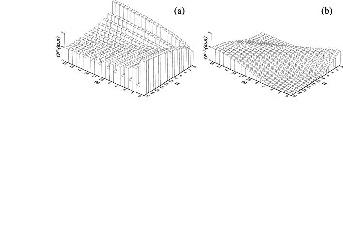
Figure 1: The coefficients $G^{(s)}(m,n)$ for (a) $s=0$, and (b) $s=-1$

For some field states the quasiprobability distribution functions ${\cal W}^{(s)}(\alpha)$ can be found in a closed form via direct integrations according to the definitions (2.45)–(2.47), and sometimes the next integration leading to the $s$-parametrized phase distributions can also be performed according to definition (2.56). In the next Sections, we shall illustrate the differences between the Pegg-Barnett phase distribution and the $s$-parametrized phase distributions obtained by integrating the $s$-parametrized quasiprobability distribution functions. For any field with known number-state matrix elements $\rho_{mn}$ of the density matrix, the $s$-parametrized phase distribution can be calculated according to eq. (2.59) with the coefficients $G^{(s)}(m,n)$ given by eq. (2.60). The distribution of the coefficients $G^{(s)}(m,n)$, for $s=0,-1$, is illustrated in fig. 1. It is apparent that for the Husimi phase distribution the coefficients decrease monotonically as we go further away from the diagonal. This means that all nondiagonal elements $\rho_{mn}$ are weighted with numbers that are less than unity, and the phase distribution for $s=-1$ is always broader than the Pegg-Barnett phase distribution (for which $G^{(s)}(m,n)\equiv 1$). For $s=0$ the situation is not so simple, because the coefficients $G^{(0)}(m,n)$ show even-odd oscillations with values that are both smaller and larger than unity. This usually leads to a phase structure sharper than the Pegg-Barnett distribution. Moreover, since the Wigner function ($s=0$) can take negative values, the positive definiteness of the Wigner phase distribution is not guaranteed. Also, the oscillatory behavior of the coefficient $G^{(0)}(m,n)$ suggests that, at least for some states, the Wigner phase distribution $P^{(0)}(\theta)$ can exhibit negative values. This nonclassical feature of $P^{(0)}(\theta)$ was shown explicitly by [Garraway and Knight [1992] [?, ?] for the simple example of the number-state superposition (only for convenience, we assume that $m>n$):

$$|\Psi\rangle = 2^{-1/2}(|n\rangle+|m\rangle).$$ (2.70)

In a straightforward manner, the general expressions for the phase distributions ${P(\theta)}$, [eq. (2.37)] and ${P^{(s)}(\theta)}$,[eq. (2.59)] reduce to

$${P(\theta)} = \frac{1}{2\pi}(1+\cos[(m-n)\theta]),$$ (2.71)

and

$${P^{(s)}(\theta)} = \frac{1}{2\pi}\left(1+G{{}^{(s)}}(m,n)\cos[(m-n)\theta]\right).$$ (2.72)

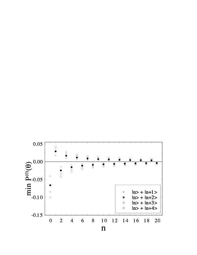
Figure 2: The minima of the Wigner phase distributions $P^{(0)}(\theta)$, eq. (2.70), for the superpositions of two number states (2.68) for various values of $n$ and $m-n$=1, 2, 3, 4.

respectively, The Pegg-Barnett, ${P(\theta)}$, and Husimi, $P^{(-1)}(\theta)$, phase distributions are obviously positive definite for any superposition (2.70). As seen in fig. 2, the Wigner phase distribution $P^{(0)}(\theta)$ is positive for superpositions with odd $m-n$. However, it takes negative values for even $m-n$. In this case, the smaller is $n$ for fixed $m-n$, or the higher is the value of $m-n$ for a given $n$, the minimum of the Wigner phase distribution is more strongly negative. Hence, one obtains the greatest negativity for the superposition $(|0\rangle+|2m\rangle)/\sqrt{2}$ in the limit of $m\rightarrow\infty$. As was emphasized by [Garraway and Knight [1993] (see also fig. 2), for large values of $n$ the Pegg-Barnett distribution is approached for both even and odd $m$.

It is highly illustrative to consider analytically the special case of eq. (2.70) when $m-n=2$ ([Garraway and Knight [1992] [?, ?]). These results will be helpful in the analysis presented in §3.2 for even and odd coherent states. Now, the coefficients $G{{}^{(s)}}(m,n)$, given by eqs. (2.60)–(2.62), can be rewritten in a much simpler form:

$$G{{}^{(s)}}(n+2,n) = \frac{1-s}{2\sqrt{(n+1)(n+2)}}\left[\left(\frac{s+1}{s-1}\right)^{n+2}-1\right]+\left(\frac{n+2}{n+1}\right)^{1/2}.$$ (2.73)

For $s=0$, eq. (2.73) goes over into ([Garraway and Knight [1992] [?, ?]):

$$G^{(0)}(n+2,n) = \left(\frac{n+2}{n+1}\right)^{(-1)^{n}/2}$$ (2.74)

and for $s=-1$ one obtains

$$G^{(-1)}(n+2,n) = \left(\frac{n+1}{n+2}\right)^{1/2}.$$ (2.75)

Equation (2.74) provides direct proof of the oscillatory behavior of $G^{(0)}(n+2,n)$ with increasing $n$. For even $n$, the right-hand-side of eq. (2.74) is greater than unity, which implies a negative minimum of the Wigner phase distribution (2.72) [solid circles in fig. 2]. However, for odd $n$, the coefficients $G^{(0)}(n+2,n)$ are less than unity and equal to $G^{(-1)}(n+2,n)$. Hence the Husimi and Wigner phase distributions for such states (with odd $n$) are equal and positive definite.

From the form of the coefficients $G^{(s)}(m,n)$ it is evident that there is no $s$ such that $G^{(s)}(m,n)=1$ for all $m$, $n$. This means that there is no “phase ordering” of the field operators; that is, the ordering for which $P{{}^{(s)}}(\theta)$ would be equal to ${P(\theta)}$. However, for a given state of the field one can find $s$ such that the two distributions are “almost identical”. Formula (2.59) is quite general, and it was used in earlier studies of the phase properties of the anharmonic oscillator [Tanaś, Gantsog, Miranowicz and Kielich [1991], parametric down conversion [Tanaś and Gantsog [1992b]), and displaced-number states [Tanaś, Murzakhmetov, Gantsog and Chizhov [1992]. A disadvantage of formula (2.59) is the fact that the numerical summations can be time consuming and even difficult to perform for field states with slowly converging number-state expansions. This, for example, is the case for highly squeezed states. In some cases, instead of using the number-state expansions, we can find analytical formulas for ${P^{(s)}(\theta)}$ via direct integrations, as shown in §3. In many cases such formulas can be treated as good approximations to the Pegg-Barnett phase distribution.

3 Phase properties of single-mode optical fields

Optical fields produced in nonlinear optical processes have specific phase properties which depend on the nonlinear process in which the field is produced and on the state of the field before it undergoes the nonlinear transformation. Since there is a large variety of nonlinear optical processes, there is the possibility to generate fields with different phase properties. Here, some examples of such field states will be given and their phase properties discussed briefly.

3.1 Coherent states

The most common single-mode field in quantum optics is a Glauber coherent state. Its phase properties have probably been analyzed within each known phase formalism. We shall focus our attention on two of them only.

The $s$-parametrized quasiprobability distribution function for a coherent state

$$|\alpha_{0}\rangle = \hat{D}(\alpha_{0})|0\rangle$$ (3.1)

can be calculated from eqs. (2.45)–(2.47) as

$${\cal W}^{(s)}(\alpha) = \frac{1}{\pi^{2}}\int\exp(\alpha\xi^{*}-\alpha^{*}\xi+s|\xi|^{2}/2)\langle 0|\hat{D}^{\dagger}(\alpha_{0})\hat{D}(\xi)\hat{D}(\alpha_{0})|0\rangle\,{\rm d}^{2}\xi$$ (3.2)

$$= \frac{1}{\pi^{2}}\int\exp[(\alpha-\alpha_{0})\xi^{*}-(\alpha^{*}-\alpha_{0}^{*})\xi+s|\xi|^{2}/2]\langle 0|\hat{D}(\xi)|0\rangle\,{\rm d}^{2}\xi$$

$$= \frac{1}{\pi^{2}}\int\exp[(\alpha-\alpha_{0})\xi^{*}-(\alpha^{*}-\alpha_{0}^{*})\xi+s|\xi|^{2}/2-|\alpha_{0}|^{2}/2]\,{\rm d}^{2}\xi$$

$$= \frac{1}{\pi}\frac{2}{1-s}\exp\left\{-\frac{2}{1-s}|\alpha-\alpha_{0}|^{2}\right\}.$$

The corresponding $s$-parametrized phase distribution is ([Tanaś, Miranowicz and Gantsog [1993]; for $s=0$ see also [Garraway and Knight [1993] and BR93):

$${P^{(s)}(\theta)} = \int\limits_{0}^{\infty}{\cal W}^{(s)}(\alpha)|\alpha|\>{\rm d}|\alpha|$$ (3.3)

$$= \frac{1}{2\pi}\exp[-(X_{0}^{2}-X^{2})]\left\{\exp(-X^{2})+\sqrt{\pi}X\,(1+{\rm erf}(X))\right\},$$

where

$$X = X{{}^{(s)}}(\theta)\>=\>\sqrt{\frac{2}{1-s}}|\alpha_{0}|\cos(\theta-\vartheta_{0}),$$ (3.4)

and $X_{0}=X{{}^{(s)}}(\vartheta_{0})$; $\vartheta_{0}$ is the phase of $\alpha_{0}$. The phase distribution $P^{(1)}(\theta)$ associated with the $P$-function can be obtained from eqs. (3.3) and (3.4) in the limit of $s\rightarrow 1$:

$$P^{(1)}(\theta) = \delta(\theta-\vartheta_{0}),$$ (3.5)

which is the Dirac delta function. This result can also be achieved from eq. (2.68). As was shown by [Miranowicz [1994], the coefficients $a_{m}^{(1)}$ are unity for arbitrary $m$. Hence, eq. (2.68) reduces to

$$P^{(1)}(\theta) = \frac{1}{2\pi}\,\left\{1+2\sum_{m=1}^{\infty}\cos[m(\theta-\vartheta_{0})]\right\}$$ (3.6)

$$\equiv \delta(\theta-\vartheta_{0}),$$

which is the desired function (3.5). This example shows that the general expression (2.59) for the $s$-parametrized phase distributions is also valid in the special case of $s$=1.

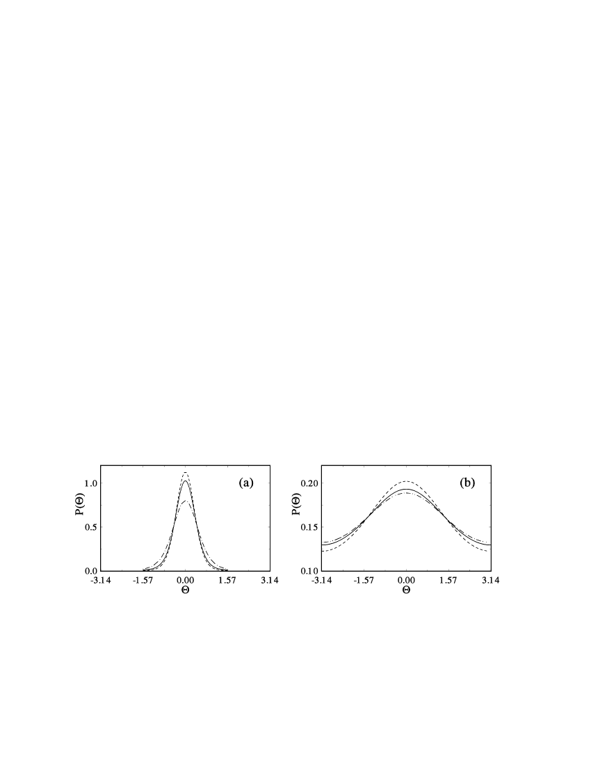
Figure 3: Phase distributions for the coherent states with the mean number of photons: (a) $|\alpha_{0}|^{2}=2$, and (b) $|\alpha_{0}|^{2}=0.01$; the Pegg-Barnett distribution (solid line), the Wigner phase function $P^{(0)}(\theta)$ (dashed line), and the Husimi phase distribution $P^{(-1)}(\theta)$ (dotted-dashed line).

Formula (3.3) is exact, it is $2\pi$-periodic, positive definite and normalized, so it satisfies all requirements for the phase distribution. Moreover, formula (3.3) has a quite simple and transparent structure. For small $|\alpha_{0}|$, the first term in braces plays an essential role, and for $|\alpha_{0}|\rightarrow 0$ we get a uniform phase distribution. For large $|\alpha_{0}|$, the second term in the braces predominates, and if we replace ${\rm erf}(X)$ by unity, we obtain the approximate asymptotic formula given by [Schleich, Dowling, Horowicz and Varro [1990] (for $s=0$):

$$P^{(0)}(\theta) \approx \sqrt{\frac{2}{\pi}}|\alpha_{0}|\cos(\theta-\vartheta_{0})\exp[-2|\alpha_{0}|^{2}\sin^{2}(\theta-\vartheta_{0})],$$ (3.7)

which however, can be applied only to $-\pi/2\leq(\theta-\vartheta_{0})\leq\pi/2$. After linearization of formula (3.7) with respect to $\theta$, the approximate formula for coherent states with large mean number of photons obtained by [Barnett and Pegg [1989] is recovered. The presence of the error function in eq. (3.3) handles properly the phase behavior in the whole range of phase values $-\pi\leq(\theta-\vartheta_{0})<\pi$.

The Pegg-Barnett distribution ${P(\theta)}$ for the coherent state $|\alpha_{0}\rangle$ can be calculated from eq. (2.36) with the superposition coefficients

$$c_{n} = b_{n}\exp({\rm i}n\vartheta_{0}),\ \ \ \ b_{n}\;=\;\exp(-|\alpha_{0}|^{2}/2)\frac{|\alpha_{0}|^{n}}{\sqrt{n!}}.$$ (3.8)

The exact formula for the $s$-parametrized phase distributions ${P^{(s)}(\theta)}$ for coherent states is given by eqs. (3.3) and (3.4). Alternatively, the ${P^{(s)}(\theta)}$ are given by eq. (2.59) after insertion of $c_{n}$ given by eq. (3.8). In fig. 3 we show the phase distributions ${P(\theta)}$, $P^{(0)}(\theta)$, and $P^{(-1)}(\theta)$ for a coherent state with the mean number of photons $|\alpha_{0}|^{2}=2$ (a), and $|\alpha_{0}|^{2}=0.01$ (b). It is seen that the Pegg-Barnett phase distribution is located somewhere between the Wigner and Husimi phase distributions. It becomes closer to $P^{(0)}(\theta)$ for $|\alpha_{0}|^{2}\gg 1$, and closer to $P^{(-1)}(\theta)$ for $|\alpha_{0}|^{2}\ll 1$. For $|\alpha_{0}|^{2}\rightarrow\infty$, the Pegg-Barnett distribution tends to the Wigner phase distribution [Schleich, Horowicz and Varro [1989a, Barnett and Pegg [1989], and for $|\alpha_{0}|^{2}\rightarrow 0$ all the distributions tend to the uniform distribution, but the Pegg-Barnett distribution in this region tends to the Husimi phase distribution. This means that for coherent states with large mean numbers of photons, $P^{(0)}(\theta)$ is a good approximation to the Pegg-Barnett phase distribution, while for small numbers of photons $P^{(-1)}(\theta)$ becomes a good approximation to the Pegg-Barnett distribution.

3.2 Superpositions of coherent states

Superpositions of macroscopically distinguishable coherent states have attracted much interest (see, for example, [Bužek and Knight [1995] and references therein) due to their property of being prototypes for the Schrödinger cats, and important nonclassical properties, such as sub-Poissonian photon statistics, quadrature squeezing, higher-order squeezing, etc.. Their phase properties have also been a subject of interest.

Let us consider the normalized superposition $|\psi\rangle$ of coherent states defined as

$$|\psi\rangle = \sum_{k=1}^{N}c_{k}|\exp({\rm i}\phi_{k})\alpha_{0}\rangle.$$ (3.9)

This superposition of two well-separated components is called a Schrödinger cat, whereas for $N>2$ the notions Schrödinger cat-like state or kitten states are often used. The phase distributions ${P(\theta)}$, [eq. (2.37)] and ${P^{(s)}(\theta)}$, [eq. (2.59)] for the state (3.9) can be rewritten in a form showing explicitly the superposition structure ([Tanaś, Gantsog, Miranowicz and Kielich [1991], [Garraway and Knight [1992] [?, ?], [Bužek, Gantsog and Kim [1993, Bužek, Kim and Gantsog [1993, Tara, Agarwal and Chaturvedi [1993, Hach III and Gerry [1993, Bužek [1993, Miranowicz [1994, Bužek and Knight [1995]).

The Pegg-Barnett phase distribution ${P(\theta)}$ splits into two terms [Tanaś, Gantsog, Miranowicz and Kielich [1991]:

$${P(\theta)} = P_{0}(\theta)\,+\,P_{\rm int}(\theta),$$ (3.10)

where

$$P_{0}(\theta) = \sum_{k=1}^{N}|c_{k}|^{2}\,P_{k}(\theta)$$ (3.11)

is the sum of phase distributions

$$P_{k}(\theta) = \frac{1}{2\pi}\left\{1+2\sum_{m>n}b_{m}b_{n}\cos\left[(m-n)(\phi_{k}+\vartheta_{0}-\theta)\right]\right\}$$ (3.12)

for the coherent states of the superposition, and the second distribution

$$P_{\rm int}(\theta) = \sum_{k,l=1\atop k\neq l}^{N}c_{k}c_{l}^{*}\,P_{kl}(\theta),$$ (3.13)

$$P_{kl}(\theta) = \frac{1}{2\pi}\sum_{m,n}b_{m}b_{n}\exp\left[{\rm i}m\,(\phi_{k}+\vartheta_{0}-\theta)-{\rm i}n\,(\phi_{l}+\vartheta_{0}-\theta)\right]$$ (3.14)

represents interference terms emerging from the quantum interference between the component states of the superposition. In fig. 4, the phase distributions (3.10) and (3.11) are presented in polar coordinates for the discrete superpositions of coherent states in the anharmonic oscillator model [see §3.5,eq. (3.57)]. It is evident from fig. 4 that as the number of components in the superposition becomes larger, the interference terms play an increasing role and the symmetry of the Pegg-Barnett distribution [eq. (3.10)] is destroyed. These terms are negligible for well-separated components of the superposition only [Tanaś, Gantsog, Miranowicz and Kielich [1991].

Analogously, the $s$-parametrized quasidistribution ${\cal W}^{(s)}(\alpha)$ for the superposition state (3.9) is represented as ([Miranowicz [1994]; for $s=-1$ see [Miranowicz, Tanaś and Kielich [1990], and for $s=0$ see also [Bužek and Knight [1995]):

$${\cal W}^{(s)}(\alpha) = {\cal W}_{0}^{(s)}(\alpha)\,+\,{\cal W}_{\rm int}^{(s)}(\alpha),$$ (3.15)

where the sum of coherent terms is

$${\cal W}_{0}^{(s)}(\alpha) = \sum_{k=1}^{N}|c_{k}|^{2}\;{\cal W}_{k}^{(s)}(\alpha)$$ (3.16)

with

$${\cal W}_{k}^{(s)}(\alpha) = \frac{1}{\pi}\frac{2}{1-s}\exp\left\{-\frac{2}{1-s}\left|\alpha-{\rm e}^{{\rm i}\phi_{k}}\alpha_{0}\right|^{2}\right\}$$ (3.17)

The interference part is given by:

$${\cal W}_{\rm int}^{(s)}(\alpha) = 2\sum_{k,l=1\atop k>l}^{N}|c_{k}|\;|c_{l}|\;{\cal W}_{kl}^{(s)}(\alpha)$$ (3.18)

with

$${\cal W}_{kl}^{(s)}(\alpha) = \frac{1}{\pi}\frac{2}{1-s}\exp\left\{-\frac{1}{1-s}\left(\left|\alpha-{\rm e}^{{\rm i}\phi_{k}}\alpha_{0}\right|^{2}+\left|\alpha-{\rm e}^{{\rm i}\phi_{l}}\alpha_{0}\right|^{2}\right)\right.$$ (3.19)

$$\quad\quad\quad\quad\quad\quad+\left.2\frac{1+s}{1-s}|\alpha_{0}|^{2}\sin^{2}\left(\frac{\phi_{k}-\phi_{l}}{2}\right)\right\}$$

$$\times\;\cos\left\{\gamma_{k}-\gamma_{l}-\frac{1+s}{1-s}|\alpha_{0}|^{2}\sin(\phi_{k}-\phi_{l})\right.$$

$$+\,\left.\frac{4}{1-s}|\alpha|\;|\alpha_{0}|\cos\left(\frac{\phi_{k}+\phi_{l}}{2}+\vartheta_{0}-\theta\right)\sin\left(\frac{\phi_{k}-\phi_{l}}{2}\right)\right\}.$$

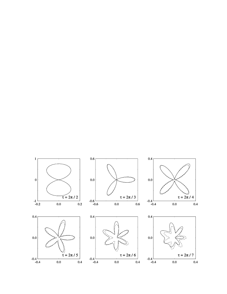
Figure 4: The Pegg-Barnett phase distributions in polar coordinates for the discrete superpositions of coherent states (3.57) with $N$=2–7 components in the anharmonic oscillator model for the initial mean photon number $|\alpha_{0}|^{2}=4$; the exact phase distributions $P(\theta)$, eq. (3.10) [solid lines], and the functions $P_{0}(\theta)$, eq. (3.11) [dashed lines], without interference contribution.

In eq. (3.19) the phases are $\gamma_{k}={\rm Arg}\,c_{k}$, $\theta={\rm Arg}\,\alpha$, $\vartheta_{0}={\rm Arg}\,\alpha_{0}$, and $\phi_{k}$ appears in the definition (3.9). On integration, we obtain the following form of the $s$-parametrized phase distribution ${P^{(s)}(\theta)}$ [Miranowicz [1994]:

$${P^{(s)}(\theta)} = P_{0}^{(s)}(\theta)\,+\,P_{\rm int}^{(s)}(\theta),$$ (3.20)

i.e., a simple sum

$$P_{0}^{(s)}(\theta) = \sum_{k=1}^{N}|c_{k}|^{2}\;P_{k}{{}^{(s)}}(\theta)$$ (3.21)

of coherent terms

$$P_{k}{{}^{(s)}}(\theta) = \frac{1}{2\pi}\exp[-(X_{0}^{2}-X_{k}^{2})]\left\{\exp(-X_{k}^{2})+\sqrt{\pi}X_{k}\;[1+{\rm erf}(X_{k})]\right\},$$ (3.22)

where

$$X_{k} = X_{kk}^{(s)}(\theta)\,=\,\sqrt{\frac{2}{1-s}}|\alpha_{0}|\cos(\theta-\vartheta_{0}-\phi_{k}),\;\;\;X_{0}\;=\;X_{kk}^{(s)}(\vartheta_{0}+\phi_{k})$$ (3.23)

and the sum

$$P_{\rm int}^{(s)}(\theta) = \sum_{k\neq l}c_{k}c_{l}^{*}P_{kl}^{(s)}(\theta)$$ (3.24)

of the interference terms

$$P_{kl}^{(s)}(\theta) = \frac{1}{2\pi}\exp[-(X^{2}_{0}\kappa_{kl}-X_{kl}^{2})]$$ (3.25)

$$\times\,\left\{\exp(-X_{kl}^{2})+\sqrt{\pi}X_{kl}\;[1+{\rm erf}(X_{kl})]\right\},$$

with

$$X_{kl}\;=\;X_{kl}^{(s)}(\theta) = \frac{1}{2}\sqrt{\frac{2}{1-s}}|\alpha_{0}|\{\exp[{\rm i}(\phi_{k}+\vartheta_{0}-\theta)]$$ (3.26)

$$+\;\exp[-{\rm i}(\phi_{l}+\vartheta_{0}-\theta)]\},$$

$$\kappa_{kl} = \frac{1-s}{2}+\frac{1+s}{2}\exp\{{\rm i}(\phi_{k}-\phi_{l})\},$$ (3.27)

The Schrödinger cat of the form:

$$|\psi\rangle \equiv |\alpha,\gamma\rangle\;=\;{\cal N}_{\gamma}\left(|\alpha\rangle+\exp({\rm i}\gamma)|-\alpha\rangle\right),$$ (3.28)

with the normalization

$${\cal N}_{\gamma} = \left[2\left(1+\cos\gamma\exp(-2|\alpha|^{2})\right)\right]^{-1/2},$$ (3.29)

is a special case of the superposition state (3.9). The cat (3.28) consists of two coherent states $|\alpha\rangle$ and $|-\alpha\rangle$, which are $\phi=\pi$ out of phase with respect to each other. The state (3.28) is not only of theoretical interest, since several methods were proposed for generation and measurement of this Schrödinger cat (e.g., [Brune, Haroche, Raimond, Davidovich and Zagury [1992, Garraway, Sherman, Moya-Cessa, Knight and Kurizki [1994]). The state $|\alpha,\pi/2\rangle$ (i.e., for $\gamma=\pi/2$) is called the Yurke-Stoler coherent state ([Yurke and Stoler [1986] [?, ?]). This state can be generated in the anharmonic oscillator model (see §3.5). For other choices of $\gamma$, the state (3.28) goes over into the even coherent state $|\alpha,0\rangle$ or the odd coherent state $|\alpha,\pi\rangle$, which have the following Fock representations [Peřina [1991]:

$$|\alpha,0\rangle = \cosh^{-1/2}(|\alpha|^{2})\sum_{n=0}^{\infty}\frac{\alpha^{2n}}{\sqrt{(2n)!}}|2n\rangle,$$ (3.30)

$$|\alpha,\pi\rangle = \sinh^{-1/2}(|\alpha|^{2})\sum_{n=0}^{\infty}\frac{\alpha^{2n+1}}{\sqrt{(2n+1)!}}|2n+1\rangle.$$ (3.31)

The dissimilar phase properties of the even/odd coherent states were analyzed by [Garraway and Knight [1993] (see also [Bužek and Knight [1995]). Their phase distributions ${P(\theta)}$ and ${P^{(s)}(\theta)}$ can be obtained readily from the general expressions (3.10) and (3.20), respectively. Obviously, they consist of the normalized sum of the phase distributions $P_{1,2}(\theta)$ (or $P_{1,2}^{(s)}(\theta)$) for coherent states located at $\alpha$ and ($-\alpha$) in the phase space plane, together with an additional interference term $P_{12}(\theta)$ (or $P_{12}^{(s)}(\theta)$). As was shown by [Garraway and Knight [1993], the Wigner phase distribution $P^{(0)}(\theta)$ for the even coherent state [eq. (3.30)] can exhibit negative values, in contrast to $P^{(0)}(\theta)$ for the odd coherent state [eq. (3.31)], which never does. The Fock expansion [eq. (3.30)] of the even coherent state contains only even photon numbers similar to the superposition $|n_{\rm even}\rangle+|n_{\rm even}+2\rangle$ discussed by us in §2.1 [see eq. (2.70) and fig. 2]. Analogously, the odd coherent state [eq. (3.31)] and $|n_{\rm odd}\rangle+|n_{\rm odd}+2\rangle$ contain only odd number states. Hence, these dissimilar features of the functions $P^{(0)}(\theta)$ for $|\alpha,0\rangle$ and $|\alpha,\pi\rangle$ are well understood for the same reasons as those given in §2.1 in the analysis of the Wigner phase distribution for the superposition of the two number states and the interpretation of the oscillatory behavior of the coefficients $G^{(0)}(m,n)$ [fig. 1a].

3.3 Squeezed states

Squeezed states have phase-sensitive noise properties, and it is particularly interesting to study their phase properties. [Sanders, Barnett and Knight [1986, Yao [1987, Loudon and Knight [1987], and [Fan and Zaidi [1988] used the Susskind-Glogower formalism in a description of the phase fluctuations of squeezed states. [Lynch [1987] applied the measured-phase formalism of [Barnett and Pegg [1986]. [Vaccaro and Pegg [1989] and [Vaccaro, Barnett and Pegg [1992] investigated phase properties of a single-mode squeezed state from the point of view of the new Pegg-Barnett phase formalism. [Grønbech-Jensen, Christiansen and Ramanujam [1989] made comparisons of the phase properties of a single-mode squeezed state obtained according to different phase formalisms, including that of Pegg and Barnett. [Burak and Wódkiewicz [1992] introduced a phase-space propensity description of quantum-phase fluctuations and analyzed, in particular, squeezed vacuum. The phase properties of the squeezed states have recently been studied by [Cohen, Ben-Aryeh and Mann [1992], and by [Collett [1993a] [?, ?]. Various measures of phase uncertainty and their dependence on the average number of photons were studied by [Freyberger and Schleich [1994].

Squeezed states (ideal squeezed states, two-photon coherent states) are defined by (see [Loudon and Knight [1987]):

$$|\alpha_{0},\zeta\rangle = \hat{D}(\alpha_{0})\hat{S}(\zeta)|0\rangle,$$ (3.32)

where $\hat{S}(\zeta)$ is the squeezing operator

$$\hat{S}(\zeta) = \exp\left(\frac{1}{2}\zeta^{*}\hat{a}^{2}-\frac{1}{2}\zeta\hat{a}^{\dagger 2}\right),$$ (3.33)

and $\zeta$ is the complex squeeze parameter

$$\zeta = r{\rm e}^{2{\rm i}\eta},\ \ \ \ r\;=\;|\zeta|.$$ (3.34)

The direct integrations lead to the $s$-parametrized quasiprobability distribution (for $\eta=0$):

$${\cal W}^{(s)}(\alpha) = \frac{2}{\sqrt{(\mu-s)(\mu^{-1}-s)}}$$ (3.35)

$$\times\;\exp\left\{-\frac{2}{\mu-s}[{\rm Im}(\alpha-\alpha_{0})]^{2}-\frac{2}{\mu^{-1}-s}[{\rm Re}(\alpha-\alpha_{0})]^{2}\right\},$$

where we have used the notation $\mu={\rm e}^{2r}$. After integration over $|\alpha|$, assuming that $\alpha_{0}$ is real, we arrive at the formula [Tanaś, Miranowicz and Gantsog [1993]:

$${P^{(s)}(\theta)} = \frac{1}{2\pi}\frac{\sqrt{(\mu-s)(\mu^{-1}-s)}}{(\mu-s)\cos^{2}\theta+(\mu^{-1}-s)\sin^{2}\theta}$$ (3.36)

$$\times\;\exp[-(X_{0}^{2}-X^{2})]\left\{\exp(-X^{2})+\sqrt{\pi}X\,(1+{\rm erf}(X))\right\},$$

where

$$X = X{{}^{(s)}}(\theta)\>=\>\sqrt{\frac{2}{\mu^{-1}-s}}\;\frac{\alpha_{0}\sqrt{\mu-s}\cos\theta}{\sqrt{(\mu-s)\cos^{2}\theta+(\mu^{-1}-s)\sin^{2}\theta}}.$$ (3.37)

Although the variable $X$ is slightly different, the main structure of the phase distribution is preserved. Formula (3.36) is valid for both small and large $\alpha_{0}$. For $\alpha_{0}=0$ we have the result for squeezed vacuum. After appropriate approximations, one easily obtains the formula derived by [Schleich, Horowicz and Varro [1989a] for a highly squeezed state.

The exact analytical formula for the $s$-parametrized phase distribution for squeezed states, as given by eqs. (3.36) and (3.37), for the squeezed vacuum takes the form:

$${P^{(s)}(\theta)} = \frac{1}{2\pi}\frac{\sqrt{(\mu-s)(\mu^{-1}-s)}}{(\mu-s)\cos^{2}\theta+(\mu^{-1}-s)\sin^{2}\theta},$$ (3.38)

where $\mu=\exp(2r)$. This formula exhibits a two-peak structure with peaks for $\theta=\pm\pi/2$ (for $r>0$). It is easy to find that the peak heights are

$$P{{}^{(s)}}(\pi/2) = \frac{1}{2\pi}\sqrt{\frac{\mu-s}{\mu^{-1}-s}},$$ (3.39)

meaning that for $s=0$, the peak height is proportional to $\mu$. One can easily check that the Pegg-Barnett result lies between the $s=0$ and $s=-1$ results. Qualitatively, all three distributions give the same two-peak phase distributions, but they differ quantitatively: the sharpest peaks are those of $P^{(0)}(\theta)$, and the broadest those of $P^{(-1)}(\theta)$.

For squeezed states with non-zero displacement $\alpha_{0}$, an additional factor of a form identical with that for coherent states, except for the different meaning of $X(\theta)$, appears in the phase distribution $P{{}^{(s)}}(\theta)$. Since this extra factor shows a peak at $\theta=0$, a competition arises between the two-peak structure of the squeezed vacuum and the one peak structure of the coherent component. This competition leads to the bifurcation in the phase distribution discussed by [Schleich, Horowicz and Varro [1989a] [?, ?]. Figure 5 illustrates such a bifurcation for $\alpha_{0}=1$, as exhibited by the Wigner and Husimi phase distributions plotted on the same scale to visualize the differences. Qualitatively, the pictures are quite similar, and differ only in the widths of the peaks. The Pegg-Barnett distribution in this case is very close to the Wigner phase distribution, and for this reason we omit it here. To calculate the Pegg-Barnett phase distribution one can apply formula (2.36) with $c_{n}$ given by (see [Loudon and Knight [1987]):

Figure 5: Pictures of the phase bifurcation for the squeezed state with the mean number of photons $|\alpha_{0}|^{2}=1$. The distributions are: (a) $P^{(0)}(\theta)$, and (b) $P^{(-1)}(\theta)$. The Pegg-Barnett distribution is very close to (a).

$$c_{n} = \langle n|\alpha_{0},\zeta\rangle\>=\>\frac{1}{\sqrt{n!\cosh r}}\left[\frac{1}{2}{\rm e}^{2{\rm i}\eta}\tanh r\right]^{n/2}H_{n}\left[\frac{\alpha_{0}+\alpha_{0}^{*}{\rm e}^{2{\rm i}\eta}\tanh r}{\sqrt{2{\rm e}^{2{\rm i}\eta}\tanh r}}\right]$$ (3.40)

$$\times\;\exp\left\{-\frac{1}{2}[|\alpha_{0}|^{2}+\alpha_{0}^{*2}{\rm e}^{2{\rm i}\eta}\tanh r]\right\},$$

assuming $\eta=0$ (results for $\eta=\pi/2$ can be obtained on replacing $r$ by $-r$).

Approximate analytical formulas for the phase variance as well as cosine and sine variances were obtained by [Vaccaro and Pegg [1989] for weakly squeezed vacuum. For large squeezing the squeezed vacuum phase variance asymptotically approaches $\pi^{2}/4$, which corresponds to the phase distribution with two symmetrically-placed delta-functions

$$P(\theta) = {1\over 2}[\delta(\theta-\pi/2)+\delta(\theta+\pi/2)].$$ (3.41)

Ideal squeezed vacuum is generated in the parametric down-conversion process, in which the pump field is treated as a constant classical quantity. Taking into account the quantum character of the pump one finds that the signal field is no longer the ideal squeezed vacuum and its phase properties are different [Tanaś and Gantsog [1992a] [see §4.5].

3.4 Jaynes-Cummings model

Figure 6: The Pegg-Barnett phase distribution (3.44) of the Jaynes-Cummings model as a function of scaled time $T=gt/(2\pi|\alpha_{0}|)$ for the initial mean photon number $|\alpha_{0}|^{2}=20$.

The Jaynes-Cummings model [Jaynes and Cummings [1963] (see reviews by [Yoo and Eberly [1985] and [Shore and Knight [1993]) is the most popular model used to describe the resonant interaction of single two-level atom with single mode of the electromagnetic field. One of the most remarkable effects predicted theoretically [Eberly, Narozhny and Sanchez-Mondragon [1980, Narozhny, Sanchez-Mondragon and Eberly [1981] and then observed experimentally [Rempe, Walther and Klein [1987] in the Jaynes-Cummings model are collapses and revivals of the atomic inversion. [Eiselt and Risken [1989], using the $Q$-function, have shown that the collapses and revivals can be understood in terms of interferences in phase space. [Phoenix and Knight [1990] mentioned the splitting of the phase probability distribution into two counter-rotating satellite distributions in a model consisting of two degenerate atomic levels, coupled through a virtual level by a Raman-type transition. [Dung, Tanaś and Shumovsky [1990] discussed the collapses and revivals in this model from the point of view of the field-mode phase properties studied in the framework of the Pegg-Barnett formalism.

The model is described by the Hamiltonian (at exact resonance):

$$\hat{H} = \hbar\omega(\hat{a}{{}^{\dagger}}\hat{a}+\hat{R}^{z})+\hbar g(\hat{R}{{}^{\dagger}}\hat{a}+\hat{R}\hat{a}{{}^{\dagger}}),$$ (3.42)

where $\hat{a}{{}^{\dagger}}$ and $\hat{a}$ are the creation and annihilation operators for the field mode; the two-level atom is described by the raising, $\hat{R}{{}^{\dagger}}$, and lowering, $\hat{R}$, operators and the inversion operator $\hat{R}^{z}$, and $g$ is the coupling constant.

To study the phase properties of the field mode, we must know the state evolution of the system. After dropping the free evolution terms, which change the phase in a trivial way, and assuming that the atom is initially in its ground state and that the field is in a coherent state $|\alpha_{0}\rangle$, the state of the system is found to be

$$|\psi(t)\rangle = \sum_{n=0}^{\infty}b_{n}\exp({\rm i}n\vartheta_{0})\left[\cos(\sqrt{n}\,gt)|n,g\rangle-{\rm i}\sin(\sqrt{n}\,gt)|n-1,e\rangle\right],$$ (3.43)

where $|g\rangle$ and $|e\rangle$ denote the ground and excited states of the atom, the coefficients $b_{n}$ are given by eq. (3.8) and $\vartheta_{0}$ is the coherent state phase.

According to the Pegg-Barnett formalism, one obtains the phase distribution ${P(\theta)}$ in the form [Dung, Tanaś and Shumovsky [1990]:

$${P(\theta)} = \frac{1}{2\pi}\left\{1+2\sum_{n>k}b_{n}b_{k}\cos[(n-k)\theta]\cos[(\sqrt{n}-\sqrt{k})gt]\right\}.$$ (3.44)

This formula can be rewritten into the form:

$${P(\theta)} = \frac{1}{2}[P_{+}(\theta)+P_{-}(\theta)],$$ (3.45)

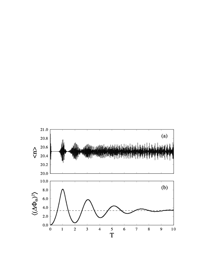
Figure 7: Evolution of (a) the mean photon number $\langle\hat{n}\rangle$ and (b) the variance $\langle(\Delta{\hat{\Phi}_{\theta}})^{2}\rangle$ of the Pegg-Barnett phase operator for the Jaynes-Cummings model as a function of scaled time $T=gt/(2\pi|\alpha_{0}|)$ for $|\alpha_{0}|^{2}=20$.

where

$$P_{\pm}(\theta) = \frac{1}{2\pi}\left\{1+2\sum_{n>k}b_{n}b_{k}\cos\left[(n-k)\theta\mp(\sqrt{n}-\sqrt{k})gt\right]\right\},$$ (3.46)

which shows explicitly that as time elapses, the phase distribution ${P(\theta)}$ splits into two distinct, right and left rotating, distributions in the polar coordinate system. Polar plots of the phase distribution are shown in fig. 6 (the time $T=gt/(2\pi|\alpha_{0}|)$ is scaled in the revival times). So, after a certain interval of time, the two counter-rotating distributions “collide”, and at that time the components of the field oscillate in phase and one can expect the revival of the atomic inversion. The numerical calculations corroborate this statement [Dung, Tanaś and Shumovsky [1990]. This behavior of the phase distribution resembles the behavior of the $Q$-function studied by [Eiselt and Risken [1991]. The time behavior of the phase variance together with the phase probability density distribution carries certain information about the collapses and revivals. To show this, we first give the explicit expression for the variance. Using eqs. (2.36) and (3.44), one obtains

$${\langle(\Delta{{\hat{\Phi}_{\theta}}})^{2}\rangle} = \frac{\pi^{2}}{3}+4\sum_{n>k}\frac{(-1)^{n-k}}{(n-k)^{2}}b_{n}b_{k}\cos[(\sqrt{n}-\sqrt{k})gt].$$ (3.47)

Variance (3.47) is illustrated graphically in fig. 7 for $|\alpha_{0}|^{2}=20$. The variance goes up initially and reaches a maximum at the scaled time $T=1$, which is the first revival time. The revival times correspond to the extrema of the phase variance. In this way, the well known phenomenon of collapses and revivals has obtained clear interpretation in terms of the cavity-mode phase. More details can be found in the paper by [Dung, Tanaś and Shumovsky [1990]. The dynamical properties of the field phase in the Jaynes-Cummings model were studied by [Dung, Tanaś and Shumovsky [1991a], and the effects of cavity damping by [Dung and Shumovsky [1992]. Some generalizations of this simple model were also considered from the point of view of their phase properties ([Dung, Tanaś and Shumovsky [1991b, Meng and Chai [1991, Meystre, Slosser and Wilkens [1991, Dung, Huyen and Shumovsky [1992, Meng, Chai and Zhang [1992, Peng and Li [1992, Peng, Li and Zhou [1992], [Wagner, Brecha, Schenzle and Walther [1992] [?, ?], [Fan [1993, Jex, Matsuoka and Koashi [1993, Drobný, Gantsog and Jex [1994, Fan and Wang [1994, Meng, Guo and Xing [1994]).

3.5 Anharmonic oscillator model

The anharmonic oscillator model is described by the Hamiltonian

$$\hat{H} = \hbar\omega\hat{a}^{\dagger}\hat{a}+{1\over 2}\hbar\kappa\hat{a}^{\dagger 2}\hat{a}^{2},$$ (3.48)

where $\hat{a}$ and $\hat{a}^{\dagger}$ are the annihilation and creation operators of the field mode, and $\kappa$ is the coupling constant, which is real and can be related to the nonlinear susceptibility $\chi^{(3)}$ of the medium if the anharmonic oscillator is used to describe propagation of laser light (with right or left circular polarization) in a nonlinear Kerr medium. If the state of the incoming beam is a coherent state $|\alpha_{0}\rangle$, the resulting state of the outgoing beam is given by

$$|\psi(\tau)\rangle = \hat{U}(\tau)|\alpha_{0}\rangle\;=\;\exp(-|\alpha_{0}|^{2}/2)\sum_{n=0}^{\infty}{\alpha_{0}^{n}\over{\sqrt{n!}}}\exp{\left[{\rm i}{\tau\over 2}n(n-1)\right]}|n\rangle,$$ (3.49)

where $\tau=-\kappa t$. In the problem of light propagating in a Kerr medium, one can make the replacement $t=-z/v$ to describe the spatial evolution of the field instead of the time evolution. On introducing the notation $\alpha_{0}=|\alpha_{0}|\exp({\rm i}\vartheta_{0})$ the state (3.49) can be written as

$$|\psi(\tau)\rangle=\sum_{n=0}^{\infty}b_{n}\exp{\left\{{\rm i}{\left[n\vartheta_{0}+{\tau\over 2}n(n-1)\right]}\right\}}|n\rangle,$$ (3.50)

where $b_{n}$ is given by eq. (3.8).

The appearance of the nonlinear phase factor in the state (3.50) modifies essentially the properties of the field represented by such a state with respect to the initial coherent state $|\alpha_{0}\rangle$. It was shown by [Tanaś [1984] that a high degree of squeezing can be obtained in the anharmonic oscillator model. Squeezing in the same process was later considered by [Kitagawa and Yamamoto [1986], who used the name crescent squeezing because of the crescent shape of the quasiprobability distribution contours obtained in the process. The evolution of the quasiprobability distribution $Q(\alpha,\alpha^{*})$ in the anharmonic oscillator model was considered by [Milburn [1986], [Milburn and Holmes [1986], [Peřinová and Lukš [1988] [?, ?], [Daniel and Milburn [1989], and [Peřinová, Lukš and Kárská [1990]. The states that differ from coherent states by extra phase factors, as in eq. (3.50), are the generalized coherent states introduced by [Titulaer and Glauber [1966] and discussed by [Stoler [1971]. [Białynicka-Birula [1968] has shown that, under appropriate periodic conditions, such states become discrete superpositions of coherent states. [Yurke and Stoler [1986], and [Tombesi and Mecozzi [1987] discussed the possibility of generating quantum-mechanical superpositions of macroscopically distinguishable states in the course of evolution for the anharmonic oscillator. [Miranowicz, Tanaś and Kielich [1990] have shown that superpositions with not only even but also odd numbers of components can be obtained.

The Pegg-Barnett Hermitian phase formalism has been applied to the study of the phase properties of the states (3.50) by [Gerry [1990], who discussed the limiting cases of very low and very high light intensities, and by [Gantsog and Tanaś [1991f], who gave a more systematic discussion of the exact results. Phase fluctuations in the anharmonic oscillator model were also analyzed within former phase formalisms ([Gerry [1987], [Lynch [1987]).

The continuous Pegg-Barnett phase probability distribution (2.36) for the field state (3.50) takes the following form:

$${P(\theta)} = {1\over{2\pi}}{\left\{1+2\sum_{n>k}b_{n}b_{k}\cos{\left[(n-k)\theta-{\tau\over 2}[n(n-1)-k(k-1)]\right]}\right\}}.$$ (3.51)

and the $s$-parametrized quasiprobability distribution function is now given by  [Miranowicz [1994]:

$${\cal W}^{(s)}(\alpha,\tau) = \frac{2}{1-s}\exp\left\{-\frac{2}{1-s}(|\alpha_{0}|^{2}+|\alpha|^{2})\right\}\mbox{\huge\{}2\exp\left(\frac{1+s}{1-s}|\alpha_{0}|^{2}\right)$$ (3.52)

$$\times\;\sum_{m>n}\frac{|\alpha|^{m-n}|\alpha_{0}|^{n+m}}{m!}\left(\frac{2}{1-s}\right)^{m-n}\left(\frac{s+1}{s-1}\right)^{n}L_{n}^{m-n}\left(\frac{4|\alpha|^{2}}{1-s^{2}}\right)$$

$$\times\;\cos\left\{(m-n)(\vartheta_{0}-\theta)+\frac{\tau}{2}[\;m(m-1)-n(n-1)\;]\right\}$$

$$+\;J_{0}({\rm i}\frac{4}{1-s}|\alpha|\;|\alpha_{0}|)\mbox{\huge\}},$$

where $J_{0}(x)$ is the Bessel function. For $\tau=0$, ${\cal W}^{(s)}(\alpha)$, given by eq. (3.52), is the coherent-state distribution [eq. (3.2)]. In the special case, for $Q$-function ($s=-1$), eq. (3.52) reduces to

$$Q(\alpha,\tau) = \exp(-|\alpha|^{2}-|\alpha_{0}|^{2})\left|\sum_{n=0}^{\infty}\frac{(\alpha^{*}\alpha_{0})^{n}}{n!}\exp\left({\rm i}\frac{\tau}{2}n(n-1)\right)\right|^{2}.$$ (3.53)

The $s$-parametrized phase distribution, resulting from eq. (3.52) is

$${P^{(s)}(\theta)} = \frac{1}{2\pi}\left\{1+2\sum_{m>n}b_{m}b_{n}\,G^{(s)}(m,n)\right.$$ (3.54)

$$\times\;\left.\cos\left[(m-n)(\theta-\vartheta_{0})-\frac{\tau}{2}\mbox{\Large(}m(m-1)-n(n-1)\mbox{\Large)}\right]\right\},$$

where the coefficients $G^{(s)}(m,n)$ are given by eq. (2.60). Symmetrization of the phase window with respect to the phase $\vartheta_{0}$ as done for the Pegg-Barnett phase distribution [eq.(3.51)] is equivalent to introduction of the relative phase variable $\theta-\vartheta_{0}$, and the two formulas differ only by the coefficients $G^{(s)}(m,n)$, as in eq. (2.59). For $\tau=0$, eqs. (3.51) and (3.54) describe the phase probability distributions for the initial coherent state $|\alpha_{0}\rangle$. When the nonlinear evolution is on ($\tau\neq 0$), the distributions ${P(\theta)}$ and ${P^{(s)}(\theta)}$ acquire some new and very interesting features. A systematic discussion of the properties as well as the plots of ${P(\theta)}$ and $P^{(-1)}(\theta)$ are given by [Tanaś, Gantsog, Miranowicz and Kielich [1991] and by [Gantsog and Tanaś [1991f].

The phase distribution ${P(\theta)}$ can be used to calculate the mean and the variance of the phase operator, defined by eqs. (2.24) and (2.25). The results are [Gantsog and Tanaś [1991f]:

$$\langle\psi(\tau)|{\hat{\Phi}_{\theta}}|\psi(\tau)\rangle=\vartheta_{0}+\int\limits_{-\pi}^{\pi}\theta{P(\theta)}\,{\rm d}\theta$$ (3.55)

$$=\vartheta_{0}-2\sum_{n>k}b_{n}b_{k}{{(-1)^{n-k}}\over{n-k}}\sin{\left\{{\tau\over 2}[n(n-1)-k(k-1)]\right\}},$$

$${\langle(\Delta{{\hat{\Phi}_{\theta}}})^{2}\rangle}=\int\limits_{-\pi}^{\pi}\theta^{2}{P(\theta)}\,{\rm d}\theta-{\left[\int\limits_{-\pi}^{\pi}\theta{P(\theta)}\,{\rm d}\theta\right]}^{2}$$ (3.56)

$$= {{\pi^{2}}\over 3}+4\sum_{n>k}b_{n}b_{k}{{(-1)^{n-k}}\over{(n-k)^{2}}}\cos{\left\{{\tau\over 2}[n(n-1)-k(k-1)]\right\}}$$

$$-\;{\left\{2\sum_{n>k}b_{n}b_{k}{{(-1)^{n-k}}\over{n-k}}\sin{\left\{{\tau\over 2}[n(n-1)-k(k-1)]\right\}}\right\}}^{2}.$$

For $\tau=0$, we recover the results for a coherent state with the phase $\vartheta_{0}$ [eqs. (2.31) and (2.39)]. The nonlinear evolution of the system leads to a nonlinear shift of the mean phase and essentially modifies the variance. An example is illustrated in fig. 8, where the evolution of the mean phase (fig. 8a) and its variance (fig. 8b) are plotted against $\tau$ for various values of $|\alpha_{0}|^{2}$. We have assumed $\vartheta_{0}=0$, and the window of the phase values is taken between $-\pi$ and $\pi$. The evolution is periodic with the period $2\pi$, so the initial values are restored for $\tau=2\pi$. Figure 8a shows the intensity-dependent phase shift. The amplitude of the mean phase oscillation becomes larger with increasing mean number of photons. The line $\pi^{2}/3$ in fig. 8b marks the variance for the state with random distribution of phase. It is seen clearly from fig. 8b that the stronger the initial field, the higher the phase variance. For $|\alpha_{0}|^{2}=4$ the phase variance increases rapidly and most of the period oscillates around $\pi^{2}/3$ – the value for uniform phase distribution. This means that the phase is randomized during the evolution, although it periodically reproduces its initial values. This tendency is even more pronounced when the mean number of photons increases. The periodicity of the evolution is destroyed by damping [Gantsog and Tanaś [1991b]. The sine and cosine functions of the phase were also calculated and the results compared with other approaches [Gantsog and Tanaś [1991f].

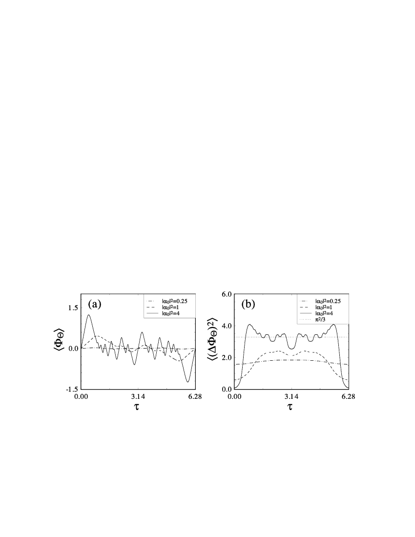
Figure 8: Evolution of (a) the mean phase (3.55) and (b) the phase variance (3.56) for the anharmonic oscillator model.

The local minima in ${\langle(\Delta{{\hat{\Phi}_{\theta}}})^{2}\rangle}$ apparent in fig. 8 indicate the points in the evolution in which superpositions of coherent states are formed, and the phase variance decreases at these points. This occurs for $\tau=2\pi M/N$ ($N$=2, 3, 4,…, and $M$, $N$ are mutually prime numbers), for which the ${P(\theta)}$ and ${P^{(s)}(\theta)}$ plotted in polar coordinates show $N$-fold symmetry, confirming the generation of discrete superpositions of coherent states with 2, 3, 4, …components:

$$\left|\psi\left(\tau=2\pi\frac{M}{N}\right)\right\rangle = \sum_{k=1}^{2N}c_{k}|\exp({\rm i}\phi_{k})\alpha_{0}\rangle,$$ (3.57)

where the phases $\phi_{k}$ are simply

$$\phi_{k} = \frac{\pi}{N}k,\hskip 56.9055ptk=1,\ldots,2N,$$ (3.58)

and the superposition coefficients $c_{k}$, representing the so-called fractional revivals, are given by ([Averbukh and Perelman [1989], [Tanaś, Gantsog, Miranowicz and Kielich [1991]):

$$c_{k} = \frac{1}{2N}\sum_{n=1}^{2N}\exp\left(-{\rm i}\frac{\pi}{N}[nk-Mn(n-1)]\right).$$ (3.59)

Such superpositions, created during the evolution of the anharmonic oscillator model, have very specific phase properties discussed in §3.2. Plots the phase distributions (3.10) and (3.11) (where $N$ should be replaced by $2N$) for the superpositions (3.58) with several components are presented in fig. 4. The phase distribution indicates the superpositions in a very spectacular way, as shown by [Tanaś, Gantsog, Miranowicz and Kielich [1991], [Gantsog and Tanaś [1991f] and [Sanders [1992] for the anharmonic oscillator model, and by [Paprzycka and Tanaś [1992] for the model with higher nonlinearities.

3.6 Displaced number states

Other states which are interesting from the point of view of their phase properties are the displaced number states $|\alpha_{0},n_{0}\rangle$ generated by the action of the displacement operator $\hat{D}(\alpha_{0})$ on a Fock state $|n_{0}\rangle$ (see [de Oliveira, Kim, Knight and Bužek [1990]);

$$|\alpha_{0},n_{0}\rangle = \hat{D}(\alpha_{0})|n_{0}\rangle.$$ (3.60)

In a special case, when $n_{0}=0$, the states (3.60) become a coherent state $|\alpha_{0}\rangle$. The $s$-parametrized quasiprobability distribution for the state (3.60) is

$${\cal W}^{(s)}(\alpha) = \frac{1}{\pi}\frac{2}{1-s}(-1)^{n}\left(\frac{1+s}{1-s}\right)^{n}$$ (3.61)

$$\times\;\exp\left\{-\frac{2}{1-s}|\alpha-\alpha_{0}|^{2}\right\}L_{n}\left(\frac{4|\alpha-\alpha_{0}|^{2}}{1-s^{2}}\right),$$

whereas the $s$-parametrized phase distribution becomes [Tanaś, Miranowicz and Gantsog [1993]:

$${P^{(s)}(\theta)} = \left(\frac{2}{1-s}\right)^{n}\sum_{k=0}^{n}\frac{(-1)^{n-k}}{k!}\left(\frac{1+s}{2}\right)^{n-k}\left(n\atop k\right)$$ (3.62)

$$\times\;\sum_{l=0}^{k}\left(k\atop l\right)\frac{N_{k-l}(2k-2l)!}{2^{2k-2l}(k-l)!}(X_{0}^{2}-X^{2})^{l}P_{k-l}(X),$$

here

$$P_{n}(X) = \frac{N_{n}^{-1}}{2\pi}\exp[-(X_{0}^{2}-X^{2})]\left\{\exp(-X^{2})\,Q_{n}(X)+\sqrt{\pi}X\,(1+{\rm erf}(X))\right\},$$ (3.63)

$$Q_{n}(X) = \frac{2^{2n}(n!)^{2}}{(2n)!}\sum_{k=0}^{n}\frac{1}{k!}X^{2k}-\sum_{k=1}^{n}\frac{2^{2k}k!}{(2k)!}X^{2k},$$ (3.64)

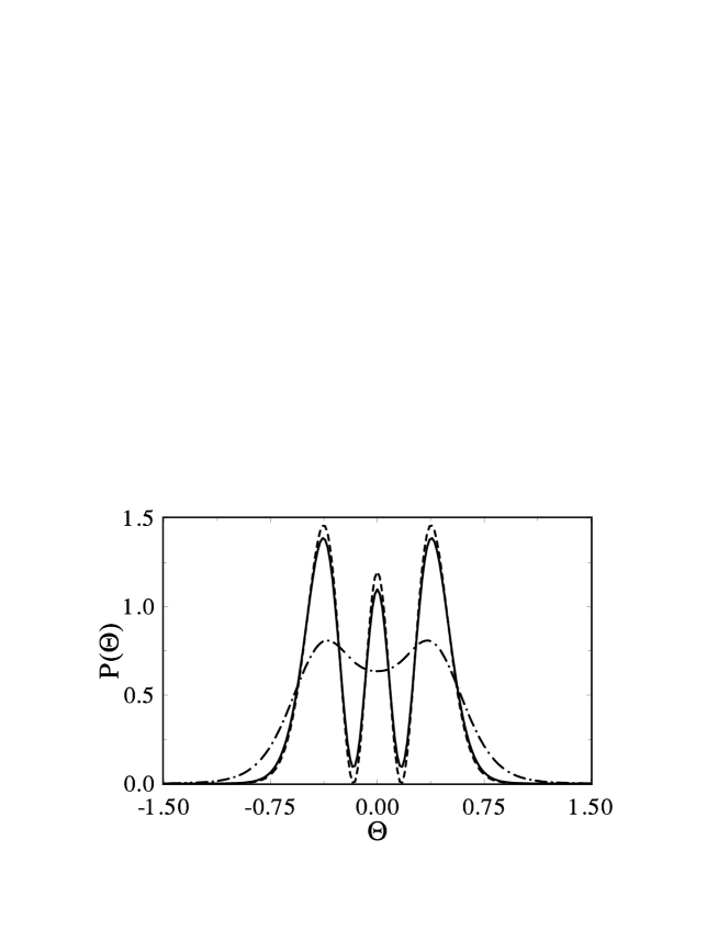
Figure 9: Phase distributions for the displaced number state with $n=2$ and $\alpha_{0}=3$. Meaning of the lines is the same as in fig. 3.

and the normalization constant is equal to

$$N_{m} = 1+\exp(-X_{0}^{2})\,\frac{1}{2\pi}\int\limits_{-\pi}^{\pi}[Q_{n}(X)-1]\,{\rm d}\theta$$ (3.65)

$$= 1+\exp(-X_{0}^{2})\left\{-1+\frac{2^{2n}(n!)^{2}}{(2n)!}\sum_{k=0}^{n}\frac{(2k)!}{2^{2k}(k!)^{3}}X_{0}^{2k}-\sum_{k=1}^{n}\frac{1}{k!}X_{0}^{2k}\right\}.$$

The $X$ variable in this case is

$$X\;=\;X{{}^{(s)}}(\theta)\;=\;\sqrt{\frac{2}{1-s}}\alpha_{0}\cos\theta,$$ (3.66)

and we have assumed $\alpha_{0}$ as real. Despite its more complex structure, formula (3.62) contains phase distributions $P_{n}(X)$ that exhibit the main features of the previous phase distributions ${P^{(s)}(\theta)}$, i.e., eq. (3.3) for a coherent state and eq. (3.36) for a squeezed state.

Displaced number states have the following Fock expansion:

$$|\alpha_{0},n_{0}\rangle = \sum_{n}b_{n}{\rm e}^{{\rm i}\phi_{n}}|n\rangle,$$ (3.67)

where the amplitudes $b_{n}$ and phase-factors $\phi_{n}$ are

$$b_{n} = \langle n|\hat{D}(|\alpha_{0}|)|n_{0}\rangle$$ (3.68)

$$= \exp\left(-\frac{1}{2}|\alpha_{0}|^{2}\right)\left(\frac{n_{-}!}{n_{+}!}\right)^{1/2}\,(-1)^{n_{+}-n}|\alpha_{0}|^{n_{+}-n_{-}}L_{n_{-}}^{n_{+}-n_{-}}(|\alpha_{0}|^{2}),$$

$$\begin{array}[]{rll}n_{-}&=&\min\{n,n_{0}\},\\ n_{+}&=&n+n_{0}-n_{-}=\max\{n,n_{0}\},\end{array}$$ (3.71)

$$\phi_{n} =\>(n-n_{0})\>{\rm Arg}\alpha_{0} =\>(n-n_{0})\vartheta_{0},$$ (3.72)

which on insertion into eq. (2.36) give explicitly the Pegg-Barnett distribution ${P(\theta)}$.

Both for coherent states and squeezed states, there was no qualitative difference between various phase distributions. Thus, one could say that at least qualitatively, all the phase distributions carried the same phase information. Here, we give an example of states for which the above statement is no longer true. These are displaced number states. The phase properties of such states were discussed earlier by [Tanaś, Murzakhmetov, Gantsog and Chizhov [1992]. It was shown that there is a qualitative difference between the Husimi phase distribution on one side, and the Pegg-Barnett and Wigner phase distributions on the other. There is an essential loss of information in the case of the Husimi phase distribution. The differences can be interpreted easily when the concept of the area of overlap in phase space introduced by [Schleich and Wheeler [1987] is invoked. Formula (3.62) provides the possibility of deeper insight into the structure of the $s$-parametrized phase distributions. The phase distribution $P{{}^{(s)}}(\theta)$ is a result of competition between the functions $P_{n}(X)$, which are peaked at $\theta=0$, and the functions $(X_{0}^{2}-X^{2})^{l}$, which have peaks at $\theta=\pm\pi/2$. For $s=-1$ only the term with $n-k=0$ survives, and there is no modulation due to the $(-1)^{n-k}$ factor. This is the reason why the Husimi phase distribution can have at most two peaks, no matter how large is $n$. Both for the Pegg-Barnett phase distribution and $P^{(0)}(\theta)$ there are $n+1$ peaks. It is also worth noting that despite the fact that the Wigner function ${\cal W}^{(0)}$, [eq. (3.61)] oscillates between positive and negative values, the Wigner phase distribution $P^{(0)}(\theta)$ [eq. (3.62)] is positive definite. An illustration of the differences between the phase distributions for the displaced number states with $n=2$ and $|\alpha_{0}|^{2}=9$ is shown in fig. 9. It is seen that the Pegg-Barnett phase distribution is very close to $P^{(0)}(\theta)$, and that they carry basically the same phase information, while there is an essential loss of phase information carried by $P^{(-1)}(\theta)$. The Pegg-Barnett and $P^{(0)}(\theta)$ distributions are very similar for given $n$, while $P^{(-1)}(\theta)$ has at most two peaks that become broader as $n$ increases. This example shows the difference between a “pure” canonical phase distribution such as the Pegg-Barnett distribution, which could be associated with a “pure” phase measurement, and a “measured” phase distribution such as $P^{(-1)}(\theta)$, which can be associated with the noisy measurement of the phase. The noise introduced by the measurement process reduces the phase information that can be inferred from the measured data.

4 Phase properties of two-mode optical fields

The single-mode version of the Pegg-Barnett phase formalism can be extended easily into the two-mode fields [Barnett and Pegg [1990] that are often a subject of consideration in quantum optics. This leads to the joint phase probability distribution for the phases of the two modes, and allows the study of not only the individual mode phase characteristics discussed above but also essentially two-mode phase characteristics such as correlation between the phases of the two modes. The phase properties of a two-mode field are simply constructed from the single-mode phases (see §2.1). The two-mode joint phase distribution is given by

$$P(\theta_{a},\theta_{b})\>=\>\lim_{\sigma\rightarrow\infty}\left(\frac{\sigma+1}{2\pi}\right)^{2}|\langle\theta_{m_{a}},\theta_{m_{b}}|f\rangle|^{2}.$$ (4.1)

This phase distribution can be applied, similar to the single-mode case, to calculations of the mean values of the phase-dependent quantities, such as individual phases, their variances, etc. We are often interested not in the individual phases corresponding to either mode, but rather in the operators or distributions representing the sum and difference of the single-mode phases, which can also be calculated using the joint phase distribution [eq. (4.1)]. However, the phase sum and difference values will cover the $4\pi$ range, and the integrations over the phase sum and difference variable should be performed over the whole range. This approach, although fully justified, is not compatible with the idea that the individual phase should be $2\pi$-periodic, and there should be a way to cast the phase sum and difference into the $2\pi$ range. Such a casting procedure was proposed by [Barnett and Pegg [1990]. The two approaches, however, give different values for the phase sum and difference variances, for example, and one should be aware of the differences. Sometimes the original calculations based on the joint phase distribution (4.1) have a more transparent interpretation, especially when one considers the intermode phase correlations. We shall adduce here examples of both approaches (the quantities obtained with the use of the casting procedure will be distinguished by the subscript $2\pi$). The casting procedure is described briefly below.

The possible eigenvalues of the phase-sum operator are

$$\theta_{m_{+}}\>=\>\theta_{0a}+\theta_{0b}+\frac{2\pi}{\sigma+1}m_{+},$$ (4.2)

where $m_{+}=0,1,\ldots,2\sigma$, and the eigenvalues of the phase-difference operator are

$$\theta_{m_{-}}\>=\>\theta_{0a}-\theta_{0b}+\frac{2\pi}{\sigma+1}m_{-},$$ (4.3)

where $m_{-}=-\sigma,-\sigma+1,\ldots,\sigma$. It is seen that the eigenvalue spectra (4.2)–(4.3) of the phase sum and difference operators have widths of $4\pi$. Since phases differing by $2\pi$ are physically indistinguishable, the phase sum and difference operators and distributions should be cast into a $2\pi$-range [Barnett and Pegg [1990]. The casting procedure can be applied to the joint continuous-phase distribution $P_{4\pi}(\theta_{+},\theta_{-})$, defined as

$$P_{4\pi}(\theta_{+},\theta_{-}) = \frac{1}{2}\lim_{\sigma\rightarrow\infty}\left(\frac{\sigma+1}{2\pi}\right)^{2}|\langle\theta_{m_{+}},\theta_{m_{-}}|f\rangle|^{2},$$ (4.4)

where

$$\theta_{\pm} = \theta_{a}\pm\theta_{b}.$$ (4.5)

As was stressed by [Barnett and Pegg [1990], there are many ways to apply the casting procedure. However, if the distribution $P_{4\pi}(\theta_{+},\theta_{-})$ is sharply peaked, we must avoid splitting the original single peak into two parts, one at each end of the $2\pi$-interval. Such a poor choice of the $2\pi$-range leads to the same interpretation problems encountered for a poor choice of $\theta_{0}$ in the single-mode case [Barnett and Pegg [1989]. The casting procedure can be applied as follows:

$$P_{2\pi}(\theta_{+},\theta_{-}) = P_{4\pi}(\theta_{+},\theta_{-})+P_{4\pi}(\theta_{+}+\delta_{1},\theta_{-}+\delta_{2}),$$ (4.6)

where the shifts $\delta_{1}$ and $\delta_{2}$ are dependent on the values of $\theta_{-}$ and $\theta_{+}$:

$$\begin{array}[]{lll}{\rm I.}&\delta_{1}=2\pi,\;\delta_{2}=0&\\ \;\;\;{\rm for}&\theta_{+}\in\langle\theta_{0_{+}}+\pi,\theta_{0_{+}}+3\pi\rangle,&\theta_{-}\in\langle|\theta_{+}-\theta_{0_{+}}-2\pi|+\theta_{0_{-}}-2\pi,\theta_{0_{-}}-\pi\rangle\\ {\rm II.}&\delta_{1}=0,\;\delta_{2}=2\pi&\\ \;\;\;{\rm for}&\theta_{-}\in\langle\theta_{0_{-}}-\pi,\theta_{0_{-}}+\pi\rangle,&\theta_{+}\in\langle|\theta_{-}-\theta_{0_{-}}|+\theta_{0_{+}},\theta_{0_{+}}+\pi\rangle\\ {\rm III.}&\delta_{1}=-2\pi,\;\delta_{2}=0&\\ \;\;\;{\rm for}&\theta_{+}\in\langle\theta_{0_{+}}+\pi,\theta_{0_{+}}+3\pi\rangle,&\theta_{-}\in\langle\theta_{0_{-}}+\pi,2\pi-|\theta_{+}-\theta_{0_{+}}-2\pi|+\theta_{0_{-}}\rangle\\ {\rm IV.}&\delta_{1}=0,\;\delta_{2}=-2\pi&\\ \;\;\;{\rm for}&\theta_{-}\in\langle\theta_{0_{-}}-\pi,\theta_{0_{-}}+\pi\rangle,&\theta_{+}\in\langle\theta_{0_{+}}+3\pi,4\pi-|\theta_{-}-\theta_{0_{-}}|+\theta_{0_{+}}\rangle.\end{array}$$ (4.15)

This analysis of four regions in the ($\theta_{+},\theta_{-}$)-plane to be cut and shifted is close to the original idea of [Barnett and Pegg [1990], and can be easily understood in a geometrical representation of the variable transformation. Moreover, as a further consequence of the $2\pi$-periodicity of eq. (4.6), one can keep the same shifts $\delta_{1}$ and $\delta_{2}$ in the whole ($\theta_{+},\theta_{-}$)-plane without distinguishing any regions. Let us only mention some of the possible simplified castings:

$$P_{2\pi}(\theta_{+},\theta_{-}) = P_{4\pi}(\theta_{+},\theta_{-})+P_{4\pi}(\theta_{+},\theta_{-}\pm 2\pi)$$ (4.16)

$$= P_{4\pi}(\theta_{+},\theta_{-})+P_{4\pi}(\theta_{+}\pm 2\pi,\theta_{-})$$

$$= P_{4\pi}(\theta_{+},\theta_{-})+P_{4\pi}(\theta_{+}\pm\pi,\theta_{-}\pm\pi)$$

$$= \ldots,$$

and combinations of the shifts satisfying the condition $|\delta_{1}|+|\delta_{2}|=2\pi$ or $||\delta_{1}|-|\delta_{2}||=2\pi$. The resulting joint distribution $P_{2\pi}(\theta_{+},\theta_{-})$ is $2\pi$-periodic in $\theta_{+}$ and $\theta_{-}$. Alternatively, one can apply the casting procedure to phase distribution (4.1):

$$P_{2\pi}(\theta_{+},\theta_{-})\>=\>\frac{1}{2}\left[P_{4\pi}\left(\frac{\theta_{+}+\theta_{-}}{2},\frac{\theta_{+}-\theta_{-}}{2}\right)+P_{4\pi}\left(\frac{\theta_{+}+\theta_{-}}{2}+\delta_{1},\frac{\theta_{+}-\theta_{-}}{2}+\delta_{2}\right)\right],$$ (4.17)

The factor $1/2$ occurring in eqs. (4.4) and (4.17) comes from the Jacobian of the transformation (4.5) for the variables. The marginal mod($2\pi$) phase-sum, $P_{2\pi}(\theta_{+})$, and phase- difference, $P_{2\pi}(\theta_{-})$, distributions are given by

$$P_{2\pi}(\theta_{\mp}) = \int\limits_{\theta^{\prime}_{0\pm}}^{\theta^{\prime}_{0\pm}+2\pi}P_{2\pi}(\theta_{+},\theta_{-}){\rm d}\theta_{\pm},$$ (4.18)

where

$$\theta^{\prime}_{0\pm} = \theta_{0\pm}\pm\pi.$$ (4.19)

In the above approach, the casting was prior to the integration. There is another equivalent manner of obtaining mod($2\pi$) marginal phase sum and difference distributions in which the casting is applied after integration. In this approach [Barnett and Pegg [1990], one starts from eq. (4.4) to calculate the $4\pi$-periodic marginal distributions $P_{4\pi}(\theta_{\pm})$:

$$P_{4\pi}(\theta_{+}) = \int\limits_{|\theta_{+}-\theta_{0_{+}}-2\pi|+\theta_{0_{-}}-2\pi}^{2\pi-|\theta_{+}-\theta_{0_{+}}-2\pi|+\theta_{0_{-}}}P_{4\pi}(\theta_{+},\theta_{-}){\rm d}\theta_{-},$$ (4.20)

$$P_{4\pi}(\theta_{-}) = \int\limits_{|\theta_{-}-\theta_{0_{-}}|+\theta_{0_{+}}}^{4\pi-|\theta_{-}-\theta_{0_{-}}|+\theta_{0_{+}}}P_{4\pi}(\theta_{+},\theta_{-}){\rm d}\theta_{+}.$$ (4.21)

Contrary to the former approach, the casting procedure is now applied to the single-mode distributions $P_{4\pi}(\theta_{\pm})$ [Barnett and Pegg [1990]:

$$P_{2\pi}(\theta_{+}) = \left\{\begin{array}[]{ll}P_{4\pi}(\theta_{+})+P_{4\pi}(\theta_{+}+2\pi)&{\rm if}\;\;\;\theta_{0_{+}}+\pi\leq\theta_{+}\leq\theta_{0_{+}}+2\pi\\ P_{4\pi}(\theta_{+})+P_{4\pi}(\theta_{+}-2\pi)&{\rm if}\;\;\;\theta_{0_{+}}+2\pi\leq\theta_{+}\leq\theta_{0_{+}}+3\pi\end{array}\right.$$ (4.24)

and

$$P_{2\pi}(\theta_{-}) = \left\{\begin{array}[]{ll}P_{4\pi}(\theta_{-})+P_{4\pi}(\theta_{-}+2\pi)&{\rm if}\;\;\;\theta_{0_{-}}-\pi\leq\theta_{-}\leq\theta_{0_{-}}\\ P_{4\pi}(\theta_{-})+P_{4\pi}(\theta_{-}-2\pi)&{\rm if}\;\;\;\theta_{0_{-}}\leq\theta_{-}\leq\theta_{0_{-}}+\pi\,.\end{array}\right.$$ (4.27)

Again, due to the $2\pi$-periodicity of $P_{2\pi}(\theta_{\pm})$ in $\theta_{\pm}$, one can simplify the recipes (4.24) and (4.27) to one of the forms:

$$P_{2\pi}(\theta_{\pm}) = P_{4\pi}(\theta_{\pm})+P_{4\pi}(\theta_{\pm}+2\pi)$$ (4.28)

$$= P_{4\pi}(\theta_{\pm})+P_{4\pi}(\theta_{\pm}-2\pi)$$

in the whole intervals $\theta_{0\pm}\leq\theta_{\pm}<\theta_{0\pm}+2\pi$.

One can analyze analogously the two-mode $s$-parametrized phase distributions. Here we give only one expression for the mod($2\pi$) $s$-parametrized phase-difference distribution for arbitrary density matrix $\hat{\rho}$ and any $s$:

$$P^{(s)}_{2\pi}(\theta_{-}) = \frac{1}{2\pi}\sum_{n=0}^{\infty}\sum_{k=0}^{n}\sum_{l=0}^{n}G^{(s)}(k,l)G^{(s)}(n-k,n-l)$$ (4.29)

$$\times\;\exp[{\rm i}(k-l)\theta_{-}]\langle l,n-l|\hat{\rho}|k,n-k\rangle$$

with the coefficients $G^{(s)}(k,l)$ given by eq. (2.60). Also, by putting $G^{(s)}(k,l)\rightarrow 1$, the mod($2\pi$) Pegg-Barnett phase-difference distribution is obtained as derived by [Luis, Sánchez-Soto and Tanaś [1995].

4.1 Two-mode squeezed vacuum

Single-mode squeezed states, discussed in §3.3, differ essentially from the two-mode squeezed states discussed extensively by [Caves and Schumaker [1985] and [Schumaker and Caves [1985]. The Pegg-Barnett phase formalism was applied by [Barnett and Pegg [1990], and by [Gantsog and Tanaś [1991g] to study the phase properties of the two-mode squeezed vacuum, and some of the results are adduced here.

The two-mode squeezed vacuum state is defined by applying the two-mode squeeze operator $\hat{S}(r,\varphi)$ on the two-mode vacuum, and is given by [Schumaker and Caves [1985]:

$$|0,0\rangle_{(r,\varphi)} = \hat{S}(r,\varphi)|0,0\rangle$$ (4.30)

$$= (\cosh r)^{-1}\exp\left(\mbox{e}^{2{\rm i}\varphi}\tanh r\>\hat{a}_{1}^{\dagger}\hat{a}_{2}^{\dagger}\right)|0,0\rangle$$

$$= (\cosh r)^{-1}\sum_{n=0}^{\infty}\left(\mbox{e}^{2{\rm i}\varphi}\tanh r\right)^{n}|n,n\rangle,$$

where $\hat{a}_{1}^{\dagger}$ and $\hat{a}_{2}^{\dagger}$ are the creation operators for the two modes, $r$ ($0\leq r<\infty$) is the strength of squeezing, and $\varphi$ ($-\pi/2\leq\varphi<\pi/2$) is the phase (note the shift in phase by $\pi/2$ with respect to the usual choice of $\varphi$).

The state (4.30), when the procedure described earlier is applied to it, leads to the joint probability distribution for the phases $\theta_{1}$ and $\theta_{2}$ of the two modes in the form [Barnett and Pegg [1990]:

$$P(\theta_{1},\theta_{2}) = (4\pi^{2}\cosh^{2}r)^{-1}\left(1+\tanh^{2}r-2\tanh r\cos(\theta_{1}+\theta_{2})\right)^{-1}.$$ (4.31)

One important property of the two-mode squeezed vacuum, which is apparent from eq. (4.31), is that $P(\theta_{1},\theta_{2})$ depends on the sum of the two phases only. Integrating $P(\theta_{1},\theta_{2})$ over one of the phases gives the marginal phase distribution $P(\theta_{1})$ or $P(\theta_{2})$ for the phase $\theta_{1}$ or $\theta_{2}$:

$$P(\theta_{1}) = \int\limits_{-\pi}^{\pi}P(\theta_{1},\theta_{2})\,{\rm d}\theta_{2}\;=\;P(\theta_{2})\;=\;\frac{1}{2\pi},$$ (4.32)

meaning that the phases $\theta_{1}$ and $\theta_{2}$ of the individual modes are distributed uniformly. This gives

$$\langle\hat{\Phi}_{\theta_{1}}\rangle = \varphi+\int\limits_{-\pi}^{\pi}\theta_{1}P(\theta_{1})\,{\rm d}\theta_{1}\;=\;\langle\hat{\Phi}_{\theta_{2}}\rangle\;=\;\varphi,$$ (4.33)

and

$$\langle\hat{\Phi}_{\theta_{1}}+\hat{\Phi}_{\theta_{2}}\rangle=2\varphi,\hskip 28.45274pt\langle\hat{\Phi}_{\theta_{1}}-\hat{\Phi}_{\theta_{2}}\rangle=0.$$ (4.34)

Thus, the phase-sum operator is related to the phase 2$\varphi$ defining the two-mode squeezed vacuum state (4.30).

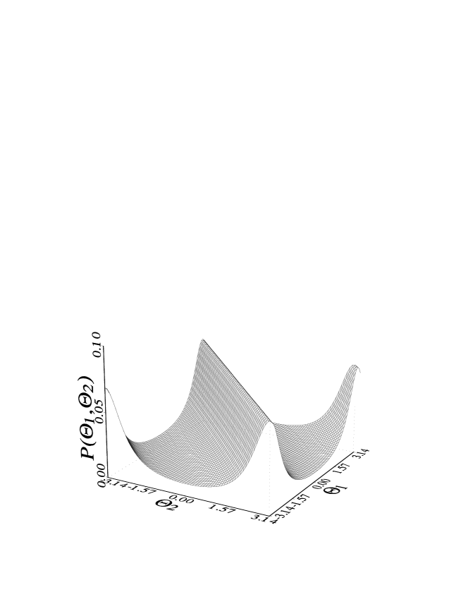
Figure 10: The joint probability distribution $P(\theta_{1},\theta_{2})$, eq. (4.19), for the two-mode squeezed vacuum with $r=0.5$.

The two-mode squeezed vacuum has very specific phase properties: the individual phases as well as the phase difference are random, and the only non-random phase is the phase sum.

Figure 10 shows an example of the joint phase probability distribution $P(\theta_{1},\theta_{2})$. The ridge, which is parallel to the diagonal of the phase window square reflects the dependence of $P(\theta_{1},\theta_{2})$ on $\theta_{1}+\theta_{2}$ only.

The phase distribution $P(\theta_{1},\theta_{2})$, [eq. (4.31)] is an explicit function of the phase sum, but not of the phase difference. This suggests expression of eq. (4.31) in new variables $(\theta_{+},\theta_{-})$. After applying the casting procedure (see introduction to §4) the joint mod($2\pi$) phase distribution is [Barnett and Pegg [1990]:

$$P_{2\pi}(\theta_{+},\theta_{-}) = (4\pi^{2}\cosh^{2}r)^{-1}\left(1+\tanh^{2}r-2\tanh r\cos\theta_{+}\right)^{-1},$$ (4.35)

whereas the marginal phase distributions are

$$P_{2\pi}(\theta_{+}) = (2\pi\cosh^{2}r)^{-1}\left(1+\tanh^{2}r-2\tanh r\cos\theta_{+}\right)^{-1},$$ (4.36)

$$P_{2\pi}(\theta_{-}) = \frac{1}{2\pi}.$$ (4.37)

The uniform shape of function (4.37) signifies randomness of the phase difference in the field [eq. (4.30)]. If the casting procedure is not applied, the marginal distributions $P(\theta_{\pm})\equiv P_{4\pi}(\theta_{\pm})$ have more complicated structures [Barnett and Pegg [1990]. In particular, $P_{4\pi}(\theta_{-})$ is not uniform because of the integration limits in eq. (4.21). In general, the mod($4\pi$) distribution has no unique shape signifying randomness of the phase sum or difference. There are many distributions in the $4\pi$-range leading to a flat mod($2\pi$) function.

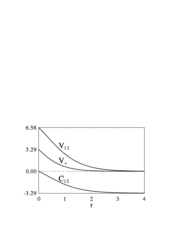
Figure 11: The phase variances $V_{12}\equiv\langle[\Delta(\hat{\Phi}_{\theta_{1}}+\hat{\Phi}_{\theta_{2}})]^{2}\rangle$, eq. (4.29), and $V_{+}\equiv\langle[\Delta(\hat{\Phi}_{\theta_{1}}+\hat{\Phi}_{\theta_{2}})]^{2}\rangle_{2\pi}$, eq. (4.30), and the phase correlation function $C_{12}$, eq. (4.28), against the squeeze parameter $r$ for the two-mode squeezed vacuum.

The two-mode variance of the phase-sum operator can be calculated according to the general formula:

$$\langle[\Delta(\hat{\Phi}_{\theta_{1}}+\hat{\Phi}_{\theta_{2}})]^{2}\rangle = {\langle(\Delta{\hat{\Phi}_{\theta_{1}}})^{2}\rangle}+{\langle(\Delta{\hat{\Phi}_{\theta_{2}}})^{2}\rangle}+2C_{12}$$ (4.38)

in terms of the individual phase variances ${\langle(\Delta{\hat{\Phi}_{\theta_{1,2}}})^{2}\rangle}$ and the phase correlation function (correlation coefficient)

$$C_{12} \equiv \langle\hat{\Phi}_{\theta_{1}}\hat{\Phi}_{\theta_{2}}\rangle-\langle\hat{\Phi}_{\theta_{1}}\rangle\langle\hat{\Phi}_{\theta_{2}}\rangle$$ (4.39)

$$= \int\limits_{-\pi}^{\pi}\int\limits_{-\pi}^{\pi}\theta_{1}\theta_{2}P(\theta_{1},\theta_{2})\,{\rm d}\theta_{1}\,{\rm d}\theta_{2}-\bigg{(}\int\limits_{-\pi}^{\pi}\theta_{1}P(\theta_{1})\,{\rm d}\theta_{1}\bigg{)}\>\bigg{(}\int\limits_{-\pi}^{\pi}\theta_{2}P(\theta_{2})\,{\rm d}\theta_{2}\bigg{)}.$$

The variances ${\langle(\Delta{\hat{\Phi}_{\theta_{1,2}}})^{2}\rangle}$ are simply $\pi^{2}/3$ [because of eq. (4.32)], and the phase correlation function $C_{12}$ is equal to:

$$C_{12} = -2(\cosh\,r)^{-2}\sum_{n>k}\frac{(\tanh\,r)^{n+k}}{(n-k)^{2}}\;=\;-2\,{\rm dilog}(1-\tanh\,r).$$ (4.40)

This correlation function describes the correlation between the phases of the two modes of the two-mode squeezed vacuum. In fig. 11 the correlation coefficient as well as the phase variances are plotted against the squeeze parameter $r$. The correlation is negative and, as $r$ tends to infinity, approaches $-\pi^{2}/3$ asymptotically. Finally, phase variance (4.38) has the form:

$$\langle[\Delta(\hat{\Phi}_{\theta_{1}}+\hat{\Phi}_{\theta_{2}})]^{2}\rangle = 2\,{\pi^{2}\over 3}-4\,{\rm dilog}(1-\tanh\,r).$$ (4.41)

The strong negative correlation between the two phases lowers the variance (4.41) of the phase-sum operator. For $r\rightarrow\infty$, this variance tends asymptotically to zero, which means that for very high squeezing the sum of the two phases becomes well defined (phase locking effect).

The (“single-mode”) mod($2\pi$) phase-sum variance is [Barnett and Pegg [1990]:

$$\langle[\Delta(\hat{\Phi}_{\theta_{1}}+\hat{\Phi}_{\theta_{2}})]^{2}\rangle_{2\pi} = \int\limits_{-\pi}^{\pi}\theta_{+}^{2}P_{2\pi}(\theta_{+}){\rm d}\theta_{+}$$ (4.42)

$$= \frac{\pi^{2}}{3}+4\,{\rm dilog}(1+\tanh\,r).$$

As the squeezing parameter $r$ varies from 0 to $\infty$, the mod($2\pi$) variance [eq. (4.42)] decreases from $\pi^{2}/3$ to zero, whereas the two-mode phase-sum variance  [eq. (4.41)] changes from $2\pi^{2}/3$ to zero with increasing $r$. Hence, both variances (4.41) and (4.42), reveal the fact that the phase sum becomes perfectly locked in the limit of large squeezing ($r\rightarrow\infty$). The value $\pi^{2}/3$ of the variance (4.42) describes random phase sum for zero squeezing. In this case of $r=0$, the two-mode variance (4.41) is twice as much as the mod($2\pi$) phase-sum variance (4.42), since it shows randomization of the two phases, $\hat{\Phi}_{\theta_{1}}$ and $\hat{\Phi}_{\theta_{2}}$, separately.

As was stressed in §4, both the original distributions, given by eqs. (4.31) and (4.32), and the mod($2\pi$) distributions, given by eqs. (4.35)–(4.37), are valid and useful. However, some care is required when interpreting the results obtained in both ways. The phase-sum variance has generally different values, as seen from fig. 11, in the two approaches. The original distributions are better for understanding the intermode phase correlation, which can be calculated explicitly from eq. (4.39), while for the mod($2\pi$) distribution the correlation is concealed in the value of the phase variance (4.42) and is not seen explicitly. On the other hand, the mod($2\pi$) results have a clear interpretation for the sum and difference of the individual phases treated as single phase variables.

Generalizing formula (2.15) and taking into account the fact that the two-mode squeezed vacuum is a “physical state”, we can calculate the expectation values of the phase exponential operators in the following way [Gantsog and Tanaś [1991g]:

$$\langle\exp({\rm i}m_{1}\hat{\Phi}_{\theta_{1}})\exp({\rm i}m_{2}\hat{\Phi}_{\theta_{2}})\rangle\;=\;\langle\widehat{\exp}({\rm i}m_{1}\Phi_{{1}{\rm SG}})\,\widehat{\exp}({\rm i}m_{2}\Phi_{{2}{\rm SG}})\rangle\hbox{}$$ (4.43)

$$= \hbox{}(\cosh r)^{-2}\sum_{n,k=0}^{\infty}\sum_{m,l=0}^{\infty}\left({\rm e}^{2{\rm i}\varphi}\tanh r\right)^{l+m}\langle l,l|n,k\rangle\langle n+m_{1},k+m_{2}|m,m\rangle$$

$$= \hbox{}\left({\rm e}^{2{\rm i}\varphi}\tanh r\right)^{m_{1}}\delta_{m_{1},m_{2}}\,,$$

where for brevity we denote $\langle(...)\rangle\>\equiv\>_{(r,\varphi)}\langle 0,0|(...)|0,0\rangle_{(r,\varphi)}$. The operators

$$\widehat{\exp}({\rm i}m_{{1},{2}}\Phi_{{1},{2}{\rm SG}}) = \sum_{n=0}^{\infty}|n\rangle\langle n+m_{{1},{2}}|$$ (4.44)

are the Susskind-Glogower phase operators for the two modes. Formula (4.43) is strikingly simple, and shows that only exponentials of the phase sum have nonzero expectation values.

Using eq. (4.43), the following results for the cosine and sine of the phase-sum operator are obtained [Gantsog and Tanaś [1991g]:

$$\langle\cos(\hat{\Phi}_{\theta_{1}}+\hat{\Phi}_{\theta_{2}})\rangle = \tanh r\cos 2\varphi,$$

$$\langle\sin(\hat{\Phi}_{\theta_{1}}+\hat{\Phi}_{\theta_{2}})\rangle = \tanh r\sin 2\varphi,$$ (4.45)

$$\langle\cos^{2}(\hat{\Phi}_{\theta_{1}}+\hat{\Phi}_{\theta_{2}})\rangle = \frac{1}{2}+\frac{1}{2}(\tanh r)^{2}\cos 4\varphi,$$

$$\langle\sin^{2}(\hat{\Phi}_{\theta_{1}}+\hat{\Phi}_{\theta_{2}})\rangle = \frac{1}{2}-\frac{1}{2}(\tanh r)^{2}\cos 4\varphi,$$ (4.46)

$$\langle[\Delta\cos(\hat{\Phi}_{\theta_{1}}+\hat{\Phi}_{\theta_{2}})]^{2}\rangle = \langle[\Delta\sin(\hat{\Phi}_{\theta_{1}}+\hat{\Phi}_{\theta_{2}})]^{2}\rangle\;=\;{1\over 2}(\cosh r)^{-2}.$$ (4.47)

For very large squeezing ($r\rightarrow\infty$, $\tanh r\rightarrow 1$, $\cosh r\rightarrow\infty$), the expectation values (4.1) and (4.1) of the functions of the phase-sum operator become asymptotically corresponding functions of the phase $2\varphi$, confirming the relation between the phase sum and $2\varphi$ that is already apparent from eq. (4.34). It is interesting that the expectation value of the phase-sum operator is equal to $2\varphi$ irrespective of the value of $r$, whereas for the sine and cosine functions correspondence is obtained only asymptotically. The variances (4.47) then become zero and the sine and cosine of the phase sum are well defined.

It should, however, be emphasized that the expectation values calculated according to the Pegg-Barnett formalism depend on the choice of the particular window of the phase eigenvalues. If a choice different from that made above were made, the clear picture of the phase properties of the two-mode squeezed vacuum would be disturbed. For example, the value of the correlation coefficient (4.40) would be different, and the phase-sum variance (4.38) would not tend asymptotically to zero. However, formulas (4.43)–(4.47), because of the way they have been calculated do not, in fact, depend on the choice of the phase window. This gives us the opportunity to make a choice which introduces consistency in the behavior of the phase itself and its sine and cosine functions. Another way of making the choice is to minimize the variance (4.38) of the phase-sum operator.

4.2 Pair coherent states

Pair coherent states introduced by [Agarwal [1986] [?, ?] are quantum states of the two-mode electromagnetic field, which are simultaneous eigenstates of the pair annihilation operator and the difference in the number operators of the two modes of the field. [Agarwal [1988] has discussed the nonclassical properties of such states, showing that they exhibit remarkable quantum features such as sub-Poissonian statistics, correlations in the number fluctuations, squeezing, and violations of the Cauchy-Schwarz inequalities. He has also presented results for fluctuations in the phase of the field using the Susskind-Glogower phase formalism. The phase properties of such states on the basis of the Pegg-Barnett formalism were studied by [Gantsog and Tanaś [1991e], and by [Gou [1993]. Phase distributions for squeezed pair coherent states were analyzed by [Gerry [1995].

The pair coherent states are defined by [Agarwal [1988] as eigenstates of the pair-annihilation operator

$$\hat{a}\hat{b}|\zeta,q\rangle = \zeta|\zeta,q\rangle,$$ (4.48)

where $\zeta$ is a complex eigenvalue and $q$ is the degeneracy parameter, which can be fixed by the requirement that $|\zeta,q\rangle$ is an eigenstate of the difference of the number operators for the two modes:

$$(\hat{a}^{\dagger}\hat{a}-\hat{b}^{\dagger}\hat{b})|\zeta,q\rangle = q|\zeta,q\rangle.$$ (4.49)

The solution to the above eigenvalue problem, assuming $q$ to be positive, is given by [Agarwal [1988]:

$$|\zeta,q\rangle=N_{q}\sum_{n=0}^{\infty}\frac{\zeta^{n}}{[n!(n+q)!]^{1/2}}|n+q,n\rangle,$$ (4.50)

where $N_{q}$ is the normalization constant

$$N_{q}=\left(\sum_{n=0}^{\infty}\frac{|\zeta|^{2n}}{n!(n+q)!}\right)^{-1/2}=[({\rm i}|\zeta|)^{-q}J_{q}(2{\rm i}|\zeta|)]^{-1/2}.$$ (4.51)

The state $|n+q,n\rangle$ is a Fock state with $n+q$ photons in mode $a$ and $n$ photons in mode $b$. If the complex number $\zeta$ is written in the form:

$$\zeta=|\zeta|\exp({\rm i}\varphi),$$ (4.52)

the state (4.50) can be written as

$$|\zeta,q\rangle=\sum_{n=0}^{\infty}b_{n}\mbox{e}^{{\rm i}n\varphi}|n+q,n\rangle,$$ (4.53)

where

$$b_{n}=N_{q}\frac{|\zeta|^{n}}{[n!(n+q)!]^{1/2}}\geq 0.$$ (4.54)

Now, the phase properties of the state (4.53) can be studied easily using the Pegg-Barnett formalism in a standard way as described above. The resulting joint probability distribution for the phases $\theta_{a}$ and $\theta_{b}$ of the two modes is given by [Gantsog and Tanaś [1991e]:

$$P(\theta_{a},\theta_{b}) = \frac{1}{(2\pi)^{2}}\biggl{\{}1+2\sum_{n>k}b_{n}b_{k}\cos[(n-k)(\theta_{a}+\theta_{b})]\biggl{\}},$$ (4.55)

where $b_{n}$ is given by eq. (4.54). For $q=0$, formula (4.55) can be written in the following simple form:

$$P(\theta_{a},\theta_{b}) = \frac{N_{0}^{2}}{(2\pi)^{2}}\exp[2|\zeta|\cos(\theta_{a}+\theta_{b})].$$ (4.56)

As in the case of the two-mode squeezed vacuum, the joint phase probability distribution depends on the sum of the two phases only, which means strong correlation between the two phases. Again, the only non-uniformly distributed phase quantity is the phase sum $\theta_{a}+\theta_{b}$. This suggests re-expression of the phase distribution (4.55) in new variables of the phase sum, $\theta_{+}=\theta_{a}+\theta_{b}$, and phase difference, $\theta_{-}=\theta_{a}-\theta_{b}$. After applying the casting procedure, the mod($2\pi$) Pegg-Barnett distribution $P_{2\pi}(\theta_{+},\theta_{-})$ takes the form:

$$P_{2\pi}(\theta_{+},\theta_{-}) = \frac{1}{4\pi^{2}}\left\{1+2\sum_{n>k}^{\infty}b_{n}b_{k}\cos[(n-k)\theta_{+}]\right\},$$ (4.57)

and the marginal distributions are:

$$P_{2\pi}(\theta_{+}) = \frac{1}{2\pi}\left\{1+2\sum_{n>k}^{\infty}b_{n}b_{k}\cos[(n-k)\theta_{+}]\right\},$$ (4.58)

and

$$P_{2\pi}(\theta_{-}) = \frac{1}{2\pi}.$$ (4.59)

For completeness of our discussion and by analogy with our presentation of the single-mode models, we now give expressions for various $s$-parametrized phase distributions. Thus, the mod($2\pi$) two-mode $s$-parametrized phase distribution is equal to

$$P^{(s)}_{2\pi}(\theta_{+},\theta_{-})\>=\>\frac{1}{4\pi^{2}}\left\{1+2\sum_{n>k}^{\infty}b_{n}b_{k}G^{(s)}(n,k)G^{(s)}(n+q,k+q)\cos[(n-k)\theta_{+}]\right\},$$ (4.60)

where the coefficients $G^{(s)}(n,k)$ are given by eqs. (2.60)–(2.62). The mod($2\pi$) marginal $s$-parametrized phase-sum distribution is

$$P^{(s)}_{2\pi}(\theta_{+}) = \frac{1}{2\pi}\left\{1+2\sum_{n>k}^{\infty}b_{n}b_{k}G^{(s)}(n,k)G^{(s)}(n+q,k+q)\cos[(n-k)\theta_{+}]\right\}.$$ (4.61)

The mod($2\pi$) $s$-parametrized phase-difference distribution $P^{(s)}_{2\pi}(\theta_{-})$ and the single-mode ones, $P^{(s)}(\theta_{a})$ and $P^{(s)}(\theta_{b})$, are uniform:

$$P^{(s)}_{2\pi}(\theta_{-}) = P^{(s)}(\theta_{a})\;=\;P^{(s)}(\theta_{b})\;=\;\frac{1}{2\pi}.$$ (4.62)

The distributions (4.60)–(4.62), similar to the distributions (4.57)–(4.59), reveal the fundamental phase properties of pair coherent states.

The correlation coefficient $C_{ab}$, eq. (4.39), [subscripts $1,2$ should be replaced by $a$ and $b$, respectively] is given in this case by the formula:

$$C_{ab} = -\,2\sum_{n>k}\frac{b_{n}b_{k}}{(n-k)^{2}},$$ (4.63)

where $b_{n}$ is given by eq. (4.54). This correlation is negative and lowers the variance of the phase-sum operator. For $|\zeta|\rightarrow\infty$, this coefficient approaches $-\pi^{2}/3$, the phase-sum variance becomes zero, and we have the classical situation of perfectly defined phase sum (the phase locking effect). This phase correlation coefficient can be contrasted with the photon number correlation coefficient, considered by [Agarwal [1988], which increases as $|\zeta|$ increases. The sine and cosine functions of the phase-sum operator were also obtained by [Gantsog and Tanaś [1991e] and compared to their counterparts obtained by [Agarwal [1988], who used the Susskind-Glogower approach.

4.3 Elliptically polarized light propagating in a nonlinear Kerr medium

To describe propagation of elliptically polarized light in a nonlinear Kerr medium, a two-mode description of the field is needed. The quantum nature of the field results in the appearance of such quantum effects as photon antibunching [Ritze and Bandilla [1979, Tanaś and Kielich [1979, Ritze [1980] and squeezing ([Tanaś and Kielich [1983] [?, ?]). [Tanaś and Kielich [1983] have shown that as much as 98 percent of squeezing can be obtained when intense light propagates in a nonlinear Kerr medium. They referred to this effect as self-squeezing. [Agarwal and Puri [1989] re-examined the problem of propagation of elliptically polarized light through a Kerr medium, considering not only the Heisenberg equations of motion for the field operators, but also the evolution of the states themselves. Quantum fluctuations in the Stokes parameters of light propagating in a Kerr medium were discussed by [Tanaś and Kielich [1990], and by [Tanaś and Gantsog [1992b].

The following effective interaction Hamiltonian can be used to describe the propagation of elliptically polarized light in a Kerr medium ([Tanaś and Kielich [1983] [?, ?]):

$$\hat{H}_{\rm I} = {1\over 2}\hbar\kappa\left(\hat{a}_{1}^{\dagger 2}\hat{a}_{1}^{2}+\hat{a}_{2}^{\dagger 2}\hat{a}_{2}^{2}+4d\hat{a}_{1}^{\dagger}\hat{a}_{2}^{\dagger}\hat{a}_{1}\hat{a}_{2}\right),$$ (4.64)

where $\hat{a}_{1}$ and $\hat{a}_{2}$ are the annihilation operators for the circularly right- (“1”) and left- (“2”) polarized modes of the field, $\kappa$ is the coupling constant, which is real and related to the nonlinear susceptibility tensor $\chi^{(3)}$ of the medium, and $d$ is the asymmetry parameter describing the coupling between the two modes. For a fully symmetrical susceptibility tensor, $d=1$. Otherwise, $d\neq 0$ and describes the asymmetry of the nonlinear properties of the medium ([Ritze [1980], [Tanaś and Kielich [1983] [?, ?]).

Using the Hamiltonian (4.64), one can obtain the evolution operator $\hat{U}(\tau)$, and assuming that the initial state of the field is a coherent state of the elliptically polarized light, one obtains for the resulting state of the field [Agarwal and Puri [1989]:

$$|\psi(\tau)\rangle = \hat{U}(\tau)|\alpha_{1},\alpha_{2}\rangle$$ (4.65)

$$= \sum_{n_{1},n_{2}}b_{n_{1}}b_{n_{2}}\exp\biggl{\{}{\rm i}(n_{1}\varphi_{1}+n_{2}\varphi_{2})$$

$$+\;{\rm i}{\tau\over 2}\left[n_{1}(n_{1}-1)+n_{2}(n_{2}-1)+4dn_{1}n_{2}\right]\biggr{\}}|n_{1},n_{2}\rangle,$$

where $\tau=n(\omega)kz/c$ ($n(\omega)$ with the refractive index), and the coefficients $b_{n_{1,2}}$ are given by eq. (3.8) with $|\alpha_{1}|^{2}$ and $|\alpha_{2}|^{2}$ as the mean numbers of photons for the circularly right- and left-polarized modes, respectively, whereas $\varphi_{1,2}$ are the phases of the coherent states of the two modes.

The state (4.65) is the two-mode state of the field, and the two-mode generalization of the Pegg-Barnett formalism used by [Gantsog and Tanaś [1991c] leads to the following joint probability distribution for the continuous-phase variables, $\theta_{1}$ and $\theta_{2}$, of the two modes:

$$P(\theta_{1},\theta_{2}) = \frac{1}{(2\pi)^{2}}\Biggl{|}\sum_{n_{1}=0}^{\infty}\sum_{n_{2}=0}^{\infty}b_{n_{1}}b_{n_{2}}\exp\biggl{\{}-{\rm i}n_{1}\theta_{1}-{\rm i}n_{2}\theta_{2}$$ (4.66)

$$+\;{\rm i}\frac{\tau}{2}[n_{1}(n_{1}-1)+n_{2}(n_{2}-1)+4dn_{1}n_{2}]\biggr{\}}\Biggl{|}^{2}.$$

The phase distribution function $P(\theta_{1},\theta_{2})$ describes the phase properties of elliptically polarized light propagating through a Kerr medium, which were discussed in detail by [Gantsog and Tanaś [1991c]. Figure 12 shows an example of the evolution of $P(\theta_{1},\theta_{2})$. It is seen that the peak is shifted and broadened during the evolution. Since the numbers of photons in the two modes are different, one can see that the shift of the peak and its broadening is asymmetric. The intensity-dependent phase shift is bigger for the mode with higher number of photons. This corresponds to the classical effect of self-phase modulation in a nonlinear Kerr medium. The quantum description shows not only the shift but also the broadening of the phase distribution (phase diffusion).

Integration of the distribution function $P(\theta_{1},\theta_{2})$ over one of the phases $\theta_{1}$ or $\theta_{2}$ leads to the marginal distribution $P(\theta_{2})$ or $P(\theta_{1})$ for the individual phases. All single-mode phase characteristics of the field can be calculated using these distributions, and the corresponding formulas were given by [Gantsog and Tanaś [1991c].

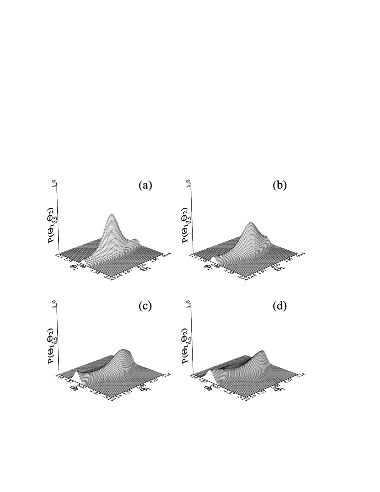
Figure 12: Evolution of the joint probability distribution $P(\theta_{1},\theta_{2})$, eq. (4.54), of light propagating in a Kerr medium: $|\alpha_{1}|^{2}=0.25$, $|\alpha_{2}|^{2}=4$ and $d=1$; (a) $\tau=0$, (b) $\tau=0.1$, (c) $\tau=0.2$, (d) $\tau=0.3$.

In addition to the phase properties of the individual modes, it is interesting, in the two-mode case, to study the behavior of the phase difference between the two modes. In the Pegg-Barnett formalism, the phase-difference operator is simply the difference of the phase operators for the two modes, so the mean value of the phase-difference operator is the difference of the mean values of the single-mode phase operators. To calculate the variance of the phase-difference operator, we can use the relation:

$$\langle[\Delta(\hat{\Phi}_{\theta_{1}}-\hat{\Phi}_{\theta_{2}})]^{2}\rangle = {\langle(\Delta{\hat{\Phi}_{\theta_{1}}})^{2}\rangle}+{\langle(\Delta{\hat{\Phi}_{\theta_{2}}})^{2}\rangle}-2C_{12},$$ (4.67)

where the last term is the correlation coefficient between the phases of the two modes and can be calculated by integration of $P(\theta_{1},\theta_{2})$ according to eq. (4.39). Thus, the resulting formula is [Gantsog and Tanaś [1991c]:

$$C_{12}(\tau)\>=\>\sum_{n_{1}>n_{1}^{\prime}}\sum_{n_{2}>n_{2}^{\prime}}f_{12}f_{21}-\left(\sum_{n_{1}=n_{1}^{\prime}}\sum_{n_{2}>n_{2}^{\prime}}f_{21}b_{n_{1}}^{2}\right)\left(\sum_{n_{2}=n_{2}^{\prime}}\sum_{n_{1}>n_{1}^{\prime}}f_{12}b_{n_{2}}^{2}\right),$$ (4.68)

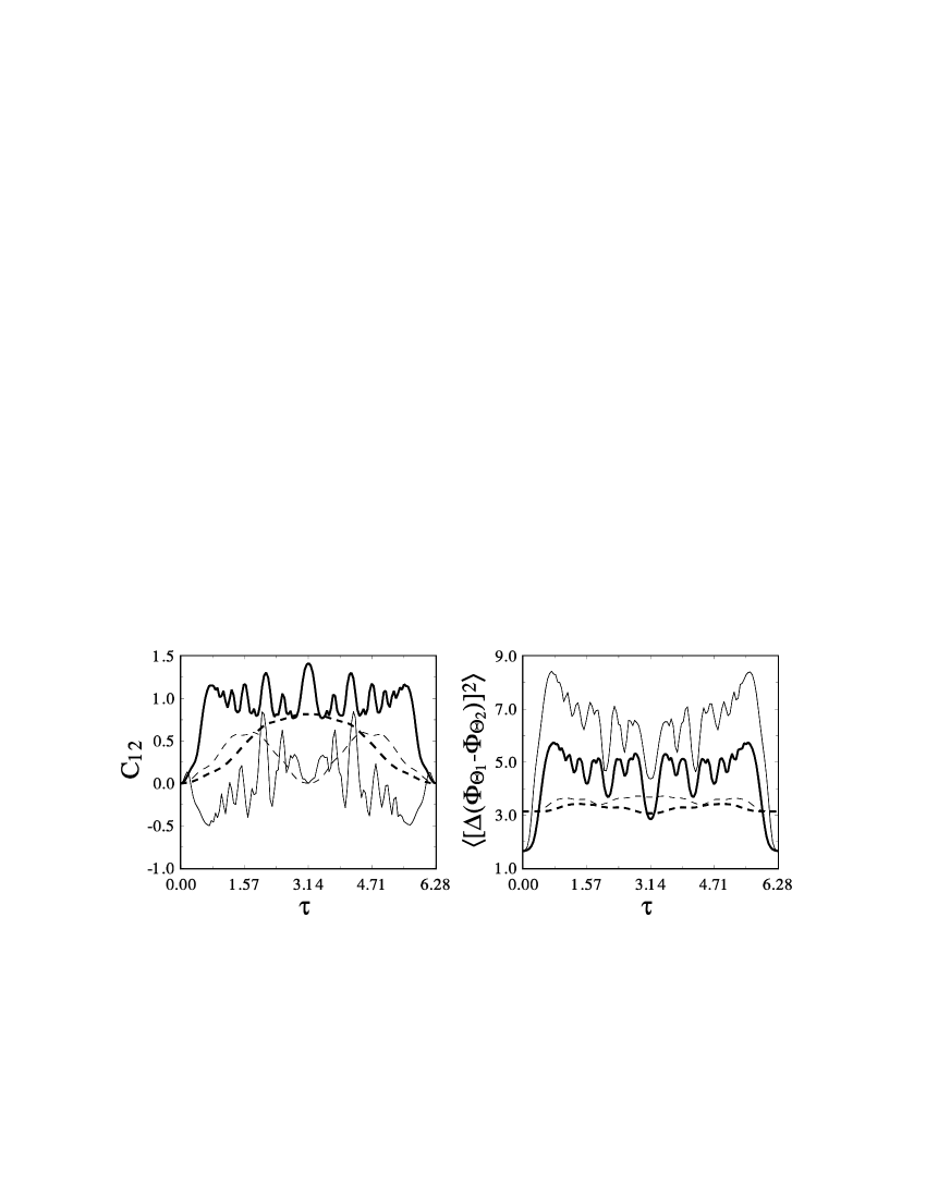
Figure 13: Evolution of the intermode phase correlation function $C_{12}(\tau)$, eq. (4.56), and the phase-difference variance $\langle[\Delta(\hat{\Phi}_{\theta_{1}}-\hat{\Phi}_{\theta_{2}})]^{2}\rangle$, eq. (4.55), of light propagating in a Kerr medium. Thin solid line: — $|\alpha_{1}|^{2}=0.25$, $|\alpha_{2}|^{2}=4$ and $d=1$; bold solid line — $|\alpha_{1}|^{2}=0.25$, $|\alpha_{2}|^{2}=4$ and $d=1/2$; thin dashed line — $|\alpha_{1}|^{2}=0.25$, $|\alpha_{2}|^{2}=0.25$ and $d=1$; bold dashed line — $|\alpha_{1}|^{2}=0.25$, $|\alpha_{2}|^{2}=0.25$ and $d=1/2$.

where

$$f_{ij} = 2b_{n_{i}}b_{n^{\prime}_{i}}\frac{(-1)^{n_{i}-n^{\prime}_{i}}}{n_{i}-n^{\prime}_{i}}\sin\left\{\frac{\tau}{2}(n_{i}-n^{\prime}_{i})\left[n_{i}+n^{\prime}_{i}-1+2d(n_{j}+n^{\prime}_{j})\right]\right\}.$$ (4.69)

A graphic illustration of the correlation function (4.68) is shown in the left-hand panel of fig. 13. The strength of the correlation depends crucially on the value of the asymmetry parameter $d$. The highest values of the correlation are obtained for $d=1/2$. This means that the minimum of the phase-difference variance, in view of eq. (4.67), is obtained for $d=1/2$. The phase-difference variance is shown in the right-hand panel of fig. 13. It was shown [Tanaś and Gantsog [1991] that, similar to the single-mode case, dissipation destroys the periodicity of the evolution and broadens the phase distribution.

Recently, the phase properties of light propagating in a Kerr medium have been reconsidered [Luis, Sánchez-Soto and Tanaś [1995] from the point of view of the Hermitian phase-difference operator introduced by [Luis and Sánchez-Soto [1994] [?, ?], which is based on the polar decomposition of the Stokes operators. This example shows clearly the difference between the Pegg-Barnett and Luis–Sánchez-Soto phase-difference formalism, which is most visible for weak fields. The Luis–Sánchez-Soto phase-difference operator differs from the Pegg-Barnett phase-difference operator, which is simply the difference of the phase operators of the two modes. For strong fields both formalisms give the same results. The nonlinear Kerr medium appears to be a good testing ground for different phase approaches.

As shown by [Gantsog and Tanaś [1991a], superpositions with any number of components can be obtained in the process of light propagation in the Kerr medium (similar to the anharmonic oscillator model described in §3.5) if the evolution time $\tau$ is taken as a fraction $M/N$ of the period, where $M$ and $N$ are mutually prime integers. Exact analytical formulas for finding the superposition coefficients were given for any $N$. The joint phase probability distribution $P(\theta_{1},\theta_{2})$ splits into separate peaks if the state of the field becomes a discrete superposition of coherent states, and this is a very spectacular way of presenting such superpositions. Some examples are shown in fig. 14.

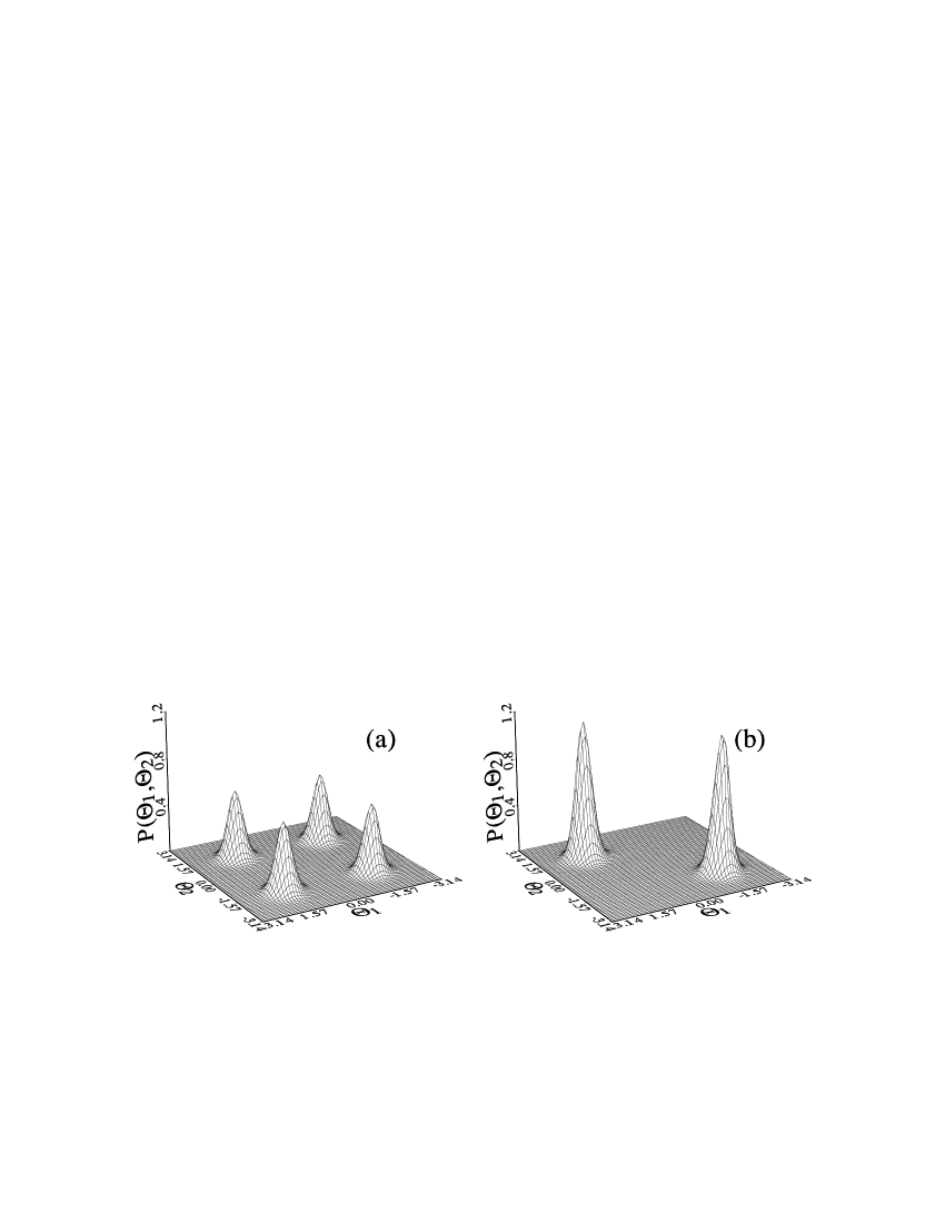
Figure 14: The joint probability distribution $P(\theta_{1},\theta_{2})$, eq. (4.54), of light propagating in a Kerr medium. $|\alpha_{1}|^{2}=|\alpha_{2}|^{2}=4$, $\tau=2\pi/2$, and (a) $d=0$; (b) $d=1/2$.

4.4 Second-harmonic generation

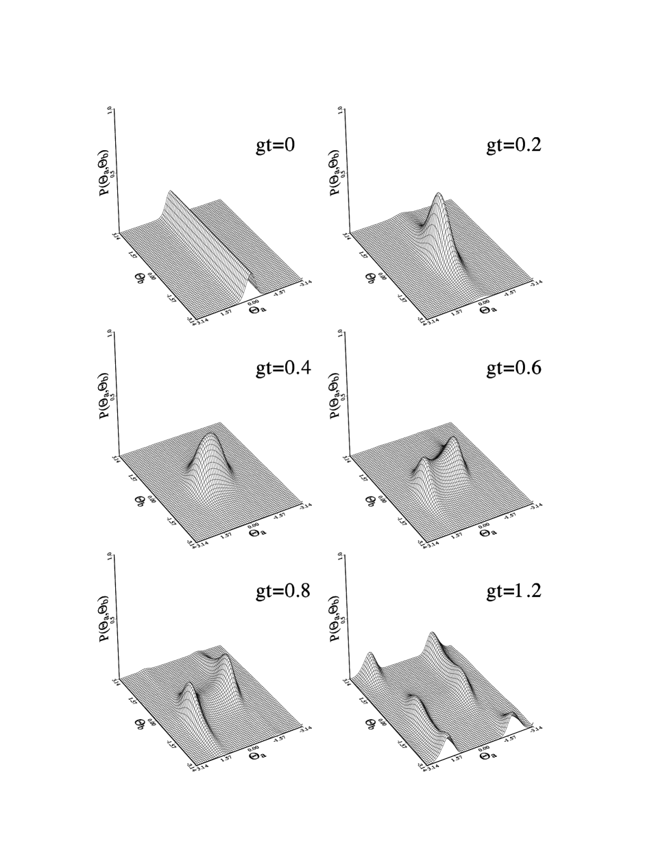
Figure 15: Evolution of the joint phase probability distribution $P(\theta_{a},\theta_{b})$, eq. (4.71), in the second-harmonic generation. The initial mean number of photons of the fundamental beam is $|\alpha_{0}|^{2}=4$, and $gt$ is the dimensionless scaled time.

Second-harmonic generation is probably the best known nonlinear optical process. In the quantum picture we deal with a nonlinear process in which two photons are annihilated and single photon with doubled frequency is created. The quantum states of the field generated in the process exhibit a number of unique quantum features such as photon antibunching [Kozierowski and Tanaś [1977] and squeezing [Mandel [1982, Wu, Kimble, Hall and Wu [1986] for both the fundamental and second-harmonic modes (for a review and literature see [Kielich, Kozierowski and Tanaś [1985]). [Nikitin and Masalov [1991] discussed the properties of the quantum state of the fundamental mode, calculating numerically the quasiprobability distribution function $Q(\alpha,\alpha^{*})$ for it. They suggested that the quantum state of the fundamental mode evolves, in the course of the second-harmonic generation, into a superposition of two macroscopically distinguishable states, similar to the superpositions obtained for the anharmonic oscillator model [Yurke and Stoler [1986, Tombesi and Mecozzi [1987, Miranowicz, Tanaś and Kielich [1990, Gantsog and Tanaś [1991f], or a Kerr medium [Agarwal and Puri [1989, Gantsog and Tanaś [1991a]. [Gantsog, Tanaś and Zawodny [1991a] discussed the phase properties of the field produced in the second-harmonic generation process.

To describe second-harmonic generation, the following model Hamiltonian is used:

$$\hat{H}\;=\;\hat{H}_{0}+\hat{H}_{\rm I} = \hbar\omega\hat{a}^{\dagger}\hat{a}+2\hbar\omega\hat{b}^{\dagger}\hat{b}+\hbar g(\hat{b}^{\dagger}\hat{a}^{2}+\hat{b}\hat{a}^{\dagger 2}),$$ (4.70)

where $\hat{a}$ ($\hat{a}^{\dagger}$) and $\hat{b}$ ($\hat{b}^{\dagger}$) are the annihilation (creation) operators of the fundamental mode of frequency $\omega$ and the second-harmonic mode at frequency $2\omega$, respectively. The coupling constant $g$, which is real, describes the coupling between the two modes. Since $\hat{H}_{0}$ and $\hat{H}_{\rm I}$ commute, there are two constants of motion: $\hat{H}_{0}$ and $\hat{H}_{\rm I}$, $\hat{H}_{0}$ determines the total energy stored in both modes, which is conserved by the interaction $\hat{H}_{\rm I}$. The free evolution can be thus factored out, and the resulting state of the field can be written as

$$|\Psi(t)\rangle = \exp(-{\rm i}\hat{H}_{\rm I}t/\hbar)|\Psi(0)\rangle,$$ (4.71)

where $|\Psi(0)\rangle$ is the initial state of the field. Since the interaction Hamiltonian $\hat{H}_{\rm I}$ is not diagonal in the number-state basis, the numerical method of diagonalization of $\hat{H}_{\rm I}$ may be applied to find the state evolution [Walls and Barakat [1970].

Let us assume that initially there are $n$ photons in the fundamental mode and no photons in the second-harmonic mode; i.e., the initial state of the field is $|n,0\rangle=|n\rangle|0\rangle$. Since $\hat{H}_{0}$ is a constant of motion, we have the relation:

$$\langle\hat{a}^{\dagger}\hat{a}\rangle+2\langle\hat{b}^{\dagger}\hat{b}\rangle = {\rm constant}\;=\;n,$$ (4.72)

which implies that the creation of $k$ photons of the second-harmonic mode requires annihilation of $2k$ photons of the fundamental mode. Thus, for given $n$, we can introduce the states

$$|\psi_{k}^{(n)}\rangle = |n-2k,k\rangle,\ \ \ \ \ \ \ \ k=0,1,\dots,[n/2],$$ (4.73)

where $[n/2]$ denotes the integer part of $n/2$, which form a complete basis of states of the field for given $n$. We have

$$\langle\psi_{k^{\prime}}^{(n^{\prime})}|\psi_{k}^{(n)}\rangle = \delta_{nn^{\prime}}\delta_{kk^{\prime}},$$ (4.74)

meaning that the constant of motion $\hat{H}_{0}$ splits the field space into orthogonal subspaces, which for given $n$ have the number of components equal to $[n/2]+1$. In such a basis, the interaction Hamiltonian has the following nonzero matrix elements:

$$\langle\psi_{k+1}^{(n)}|\hat{H}_{\rm I}|\psi_{k}^{(n)}\rangle\;\equiv\;\left(\hat{H}_{\rm I}\right)_{k+1,k}^{(n)} = \langle\psi_{k}^{(n)}|\hat{H}_{\rm I}|\psi_{k+1}^{(n)}\rangle\;\equiv\;\left(\hat{H}_{\rm I}\right)_{k,k+1}^{(n)}$$ (4.75)

$$= \hbar g\sqrt{(k+1)(n-2k)(n-2k-1)},$$

which form a symmetric matrix of the dimension $([n/2]+1)\times([n/2]+1)$ with real nonzero elements (we have assumed $g$ real) located on the two diagonals immediately above and below the principal diagonal. Such a matrix can be easily diagonalized numerically [Walls and Barakat [1970].

To find the state evolution, we need the matrix elements of the evolution operator:

$$d_{n,k}(t) \equiv \langle\psi_{k}^{(n)}|\exp(-{\rm i}\hat{H}_{\rm I}t/\hbar)|\psi_{0}^{(n)}\rangle.$$ (4.76)

If the matrix $\hat{U}$ is the unitary matrix that diagonalizes the interaction Hamiltonian matrix given by eq. (4.75), i.e.:

$$\hat{U}^{-1}\hat{H}_{\rm I}^{(n)}\hat{U} = \hbar g\times{\rm diag}\left(\lambda_{0},\lambda_{1},\ldots,\lambda_{[n/2]}\right),$$ (4.77)

then the coefficients $d_{n,k}(t)$ can be written as

$$d_{n,k}(t) = \sum_{i=0}^{[n/2]}e^{-{\rm i}gt\lambda_{i}}U_{ki}U_{0i}^{*},$$ (4.78)

where $\lambda_{i}$ are the eigenvalues of the interaction Hamiltonian in units of $\hbar g$. Of course, the matrix $\hat{U}$ as well as the eigenvalues $\lambda_{i}$ are defined for given $n$ and should have the additional index $n$, which we have omitted to shorten the notation. Moreover, for real $g$ the interaction Hamiltonian matrix is real, and the transformation matrix $\hat{U}$ is a real orthogonal matrix, so the asterisk can also be dropped.

The numerical diagonalization procedure gives the eigenvalues $\lambda_{i}$ as well as the elements of the matrix $\hat{U}$, and thus the coefficients $d_{n,k}(t)$ can be calculated according to eq. (4.78). It is worthwhile to note, however, that due to the symmetry of the Hamiltonian the eigenvalues $\lambda_{i}$ are distributed symmetrically with respect to zero, with single eigenvalue equal to zero if there is an odd number of them. When the eigenvalues are numbered from the lowest to the highest value, there is an additional symmetry relation:

$$U_{ki}U_{0i} = (-1)^{k}U_{k,[n/2]-i}U_{0,[n/2]-i}\,,$$ (4.79)

which makes the coefficients $d_{n,k}(t)$ either real ($k$ even) or imaginary ($k$ odd). This property of the coefficients $d_{n,k}(t)$ is very important and in some cases allows exact analytical results to be obtained.

With the coefficients $d_{n,k}(t)$ available, the resulting state of the field (4.71) can be written, for the initial state $|n,0\rangle$, as

$$|\psi^{(n)}(t)\rangle = \sum_{k=0}^{[n/2]}d_{n,k}(t)|\psi_{k}^{(n)}\rangle.$$ (4.80)

The typical initial conditions for the second-harmonic generation are: a coherent state of the fundamental mode and the vacuum of the second-harmonic mode. The initial state of the field can thus be written as

$$|\psi(0)\rangle = \sum_{n=0}^{\infty}c_{n}|n,0\rangle,$$ (4.81)

where $c_{n}=b_{n}{\rm e}^{{\rm i}n\varphi_{a}}$ is the Poissonian weighting factor (3.8) of the coherent state $|\alpha_{0}\rangle$ with the phase $\varphi_{a}={\rm Arg}\,\alpha_{0}$. With these initial conditions, the resulting state (4.71) is given by

$$|\psi(t)\rangle = \sum_{n=0}^{\infty}c_{n}|\psi^{(n)}(t)\rangle\;=\;\sum_{n=0}^{\infty}c_{n}\sum_{k=0}^{[n/2]}d_{n,k}(t)|n-2k,k\rangle.$$ (4.82)

Equation (4.82), describing the evolution of the system is the starting point for a further discussion of second-harmonic generation. If the initial state of the fundamental mode is not a coherent state, but has a decomposition into number states of the form (4.81) with different amplitudes $c_{n}$, eq. (4.82) is still valid if appropriate $c_{n}$’s are taken. This is true, for example, for an initially squeezed state of the fundamental mode. The coefficients $d_{n,k}(t)$ have been calculated numerically to find the evolution of the field state (4.71), and consequently, its phase properties ([Tanaś, Gantsog and Zawodny [1991a] [?, ?],  [Gantsog, Tanaś and Zawodny [1991a]).

Repeating the standard procedure of the Pegg-Barnett formalism with the field state (4.71), the joint phase probability distribution is obtained in the form:

$$P(\theta_{a},\theta_{b})\>=\>{1\over{(2\pi)^{2}}}\Biggl{|}\sum_{n=0}^{\infty}b_{n}\sum_{k=0}^{[n/2]}d_{n,k}(t)\exp\{-{\rm i}[(n-2k)\theta_{a}+k\theta_{b}-k(2\varphi_{a}-\varphi_{b})]\}\Biggr{|}^{2},$$ (4.83)

where $\theta_{a}$ and $\theta_{b}$ are continuous-phase variables for the fundamental and second-harmonic modes, and the phases $\varphi_{a}$ and $\varphi_{b}$ are the initial phases with respect to which the distribution is symmetrized. It is interesting, that formula (4.83) depends, in fact, on the difference $2\varphi_{a}-\varphi_{b}$, which reproduces the classical phase relation for second-harmonic generation. Classically, for the initial conditions chosen here, this phase difference takes the value $\pi/2$, which turns out to be a good choice to fix the phase windows in the quantum description as well.

The evolution of the joint probability distribution $P(\theta_{a},\theta_{b})$, given by eq. (4.83), is illustrated graphically in fig. 15. At the initial stage of the evolution the phase distribution in the $\theta_{a}$ direction (fundamental mode) is broadened, while a peak of the second-harmonic mode phase starts to grow. The emergence of the peak at $\theta_{b}=0$ confirms the classical relation $2\varphi_{a}-\varphi_{b}=\pi/2$, which has been applied to fix the phase window. The phase distribution in the $\theta_{b}$ direction narrows at the beginning of the evolution, meaning less uncertainty in the phase of the second harmonic. However, for later times the distribution $P(\theta_{a},\theta_{b})$ splits into two peaks, which resembles the splitting of the $Q(\alpha,\alpha^{*})$ function found by [Nikitin and Masalov [1991]. For still later times, more and more peaks appear in the distribution $P(\theta_{a},\theta_{b})$, and this distribution becomes more and more uniform, which means randomization of the phase. The route to the random phase distribution, however, goes through a sequence of increasing numbers of peaks. The splitting of the joint phase distribution can be understood if one realizes that the mean number of photons of the second harmonic oscillates and after reaching the maximum the second-harmonic generation becomes, as a matter of fact, the down-conversion process which exhibits a two-peak structure of the phase distribution in the direction of the fundamental mode (see §4.5). The appearance of new peaks may thus be interpreted as a transition of the process from the second-harmonic to the down-conversion regime, and vice versa. The phase variances for both modes tend asymptotically to the value $\pi^{2}/3$ of the randomly distributed phase [Gantsog, Tanaś and Zawodny [1991a]; however, it has turned out that partial revivals of the phase structure can be observed during the evolution [Drobný and Jex [1992].

It is also interesting to study the phase distribution of the field produced by second-harmonic generation with other than coherent initial states of the fundamental mode. Such studies were performed by [Tanaś, Gantsog and Zawodny [1991b], showing for example that even for a second harmonic generated by an initial number state the joint phase probability distribution has a modulation structure owing to the intermode correlation that develops in the process of the evolution.

4.5 Parametric down conversion with quantum pump

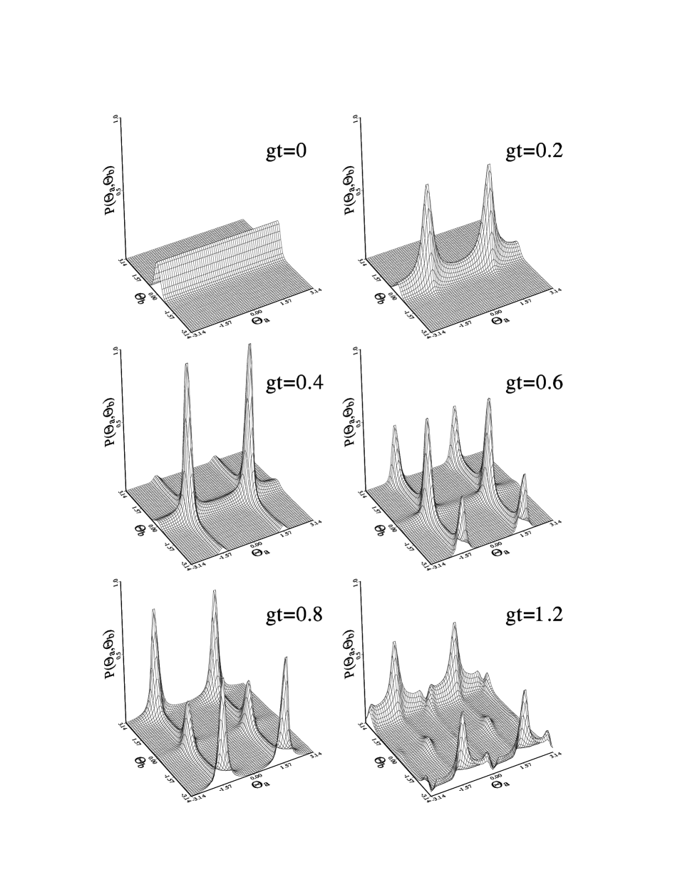
Figure 16: Evolution of the joint phase probability distribution $P(\theta_{a},\theta_{b})$, eq. (4.76), in the process of parametric down conversion with quantum pump. The initial mean number of photons in the mode $b$ is $|\beta_{0}|^{2}=4$.

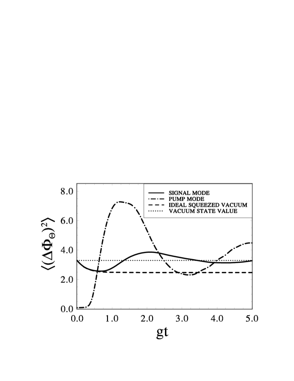
Figure 17: Evolution of the phase variances $\langle(\Delta{\hat{\Phi}_{\theta_{a}}})^{2}\rangle$, eq. (4.77), and $\langle(\Delta{\hat{\Phi}_{\theta_{b}}})^{2}\rangle$, eq. (4.78), in the parametric down conversion. The initial mean number of photons in the mode $b$ is $|\beta_{0}|^{2}=4$.

The parametric down-conversion process with quantum pump, which is a subharmonic generation process, can be described by the same model Hamiltonian, [eq. (4.70)] as the second-harmonic generation. The initial conditions distinguishing the two processes are the following: For the subharmonic generation process mode $b$ is initially populated while mode $a$ is in the vacuum state. The distinction between the two processes is far from trivial, and the states generated in the two processes have quite different properties ([Gantsog, Tanaś and Zawodny [1991b, Jex, Drobný and Matsuoka [1992],[Tanaś and Gantsog [1992a] [?, ?], [Gantsog, Tanaś and Zawodny [1993]).

Let us assume, in analogy to our analysis of second-harmonic generation, that initially there are $n$ photons in the pump mode $(b)$ and no photons in the signal mode $(a)$; i.e., the initial state of the field is $|0,n\rangle=|0\rangle_{a}|n\rangle_{b}$. Since $\hat{H}_{0}$ is a constant of motion, we have the relation

$$\langle\hat{a}^{\dagger}\hat{a}\rangle+2\langle\hat{b}^{\dagger}\hat{b}\rangle = {\rm constant}\;=\;2n,$$ (4.84)

which implies that the annihilation of $k$ photons of the pump mode requires creation of $2k$ photons of the signal mode. Thus, for given $n$, we can introduce the states

$$|\psi_{n-k}^{(2n)}\rangle = |2k,n-k\rangle,\ \ \ \ \ \ \ \ k=0,1,\ldots,n\ ,$$ (4.85)

which should be compared to the corresponding expression (4.73) for the second-harmonic generation.

Proceeding along the same lines as in second-harmonic generation, the resulting state of the field can be written as

$$|\psi(t)\rangle = \sum_{n=0}^{\infty}b_{n}\mbox{e}^{{\rm i}n\varphi_{b}}\sum_{k=0}^{n}d_{2n,k}(t)|2k,n-k\rangle,$$ (4.86)

where the coefficients $d_{2n,k}(t)$ are given by

$$d_{2n,k}(t) \equiv \langle 2k,n-k|\exp(-{\rm i}\hat{H}_{\rm I}t)\,|0,n\rangle,$$ (4.87)

whereas now the $c_{n}=b_{n}{\rm e}^{{\rm i}n\varphi_{b}}$ are the Poissonian weighting factors (3.8) for the initially coherent state $|\beta_{0}=|\beta_{0}|\exp{({\rm i}\varphi_{b})}\rangle$ of the mode $b$. Again, the method of numerical diagonalization is used to calculate the coefficients $d_{2n,k}(t)$ and, in effect, the phase properties of the state (4.86).

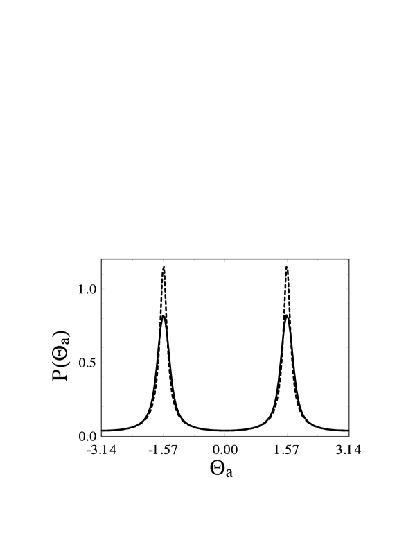
Figure 18: Phase distribution $P(\theta_{a})$, eq. (4.79), for $gt=0.3$, in the parametric down conversion.

The joint phase probability distribution in this case is given by

$$P(\theta_{a},\theta_{b})\>=\>{1\over{(2\pi)^{2}}}\Biggl{|}\sum_{n=0}^{\infty}b_{n}\sum_{k=0}^{n}d_{2n,k}(t)\exp\{-{\rm i}[2k\theta_{a}+(n-k)\theta_{b}+k(2\varphi_{a}-\varphi_{b})]\}\Biggr{|}^{2}.$$ (4.88)

As for the second-harmonic generation, we similarly take $2\varphi_{a}-\varphi_{b}=\pi/2$ to fix the phase windows. The evolution of the joint probability distribution $P(\theta_{a},\theta_{b})$ for parametric down conversion with the mean number of photons $|\beta_{0}|^{2}=4$ is shown in fig. 16. Comparison of figs. 15 and 16 shows immediately a striking difference between the phase properties of the fields obtained in the two processes. The state produced in the down-conversion process acquires from the very beginning the two-peak structure in the $\theta_{a}$ direction, which suggests the appearance of a superposition of two states in the resulting field. The two peaks which appear at the beginning of the evolution correspond, in fact, to the two-peak phase distribution of the squeezed states (see §3.3). At later stages of the evolution randomization of the two phases takes place, similarly as for the second-harmonic. However, the symmetry with respect to $\theta_{a}$ is preserved. The two-peak structure of the phase distribution has already appeared, although not in its pure form, in the phase distribution for second harmonic generation (fig. 15). Its appearance can be ascribed to the down-conversion process that has overcome second-harmonic generation at this stage of the evolution. The transition from the one-peak phase distribution to the two-peak distribution makes a qualitative difference between the two field states, and is a sort of “phase transition”.

Once the joint phase distribution $P(\theta_{a},\theta_{b})$ is known, all quantum-mechanical phase expectation values can be calculated. In particular, the phase variance for the signal mode can be calculated according to the formula:

$${\langle(\Delta{\hat{\Phi}_{\theta_{a}}})^{2}\rangle} = \int\limits_{-\pi}^{\pi}{\rm d}\theta_{a}\;\theta_{a}^{2}\int\limits_{-\pi}^{\pi}\,{\rm d}\theta_{b}\;P(\theta_{\rm a},\theta_{b})$$ (4.89)

$$= \frac{\pi^{2}}{3}+\mbox{Re}\sum_{n>n^{\prime}}b_{n}b_{n^{\prime}}\frac{\exp[-{\rm i}(n-n^{\prime})(2\varphi_{\rm a}-\varphi_{b})]}{(n-n^{\prime})^{2}}$$

$$\times\;\sum_{k=0}^{n^{\prime}}d_{2n,k+n-n^{\prime}}(t)d_{2n^{\prime},k}^{*}(t),$$

and for the pump mode we have

$${\langle(\Delta{\hat{\Phi}_{\theta_{b}}})^{2}\rangle} = \int\limits_{-\pi}^{\pi}{\rm d}\theta_{b}\;\theta_{b}^{2}\int\limits_{-\pi}^{\pi}\,{\rm d}\theta_{a}\;P(\theta_{a},\theta_{b})$$ (4.90)

$$= \frac{\pi^{2}}{3}+4\mbox{Re}\sum_{n>n^{\prime}}b_{n}b_{n^{\prime}}\frac{(-1)^{n-n^{\prime}}}{(n-n^{\prime})^{2}}\sum_{k=0}^{n^{\prime}}d_{2n,k}(t)d_{2n^{\prime},k}^{*}(t),$$

where we have used eq. (4.88), and we take $2\varphi_{a}-\varphi_{b}=\pi/2$. The time evolution of the phase variances can be calculated numerically using these expressions for given initial field states. The dynamical behavior of the phase variances calculated from eqs. (4.89) and (4.90) is illustrated graphically in fig. 17 for $|\beta_{0}|^{2}=4$. The dashed line $\pi^{2}/3$ marks the variance for the state with random distribution of phase. It is apparent that the phase variance of the signal mode starts from the value $\pi^{2}/3$, dips into the minimum, and after a few oscillations again becomes close to $\pi^{2}/3$. For comparison, the phase variance for the ideal squeezed state is also shown. The two variances are initially indistinguishable, but the phase variance for the squeezed state approaches monotonically its asymptotical value $\pi^{2}/4$, while for the quantum-pump case the phase variance of the signal mode begins to oscillate at later times. This confirms the statement that there a limit is imposed by the quantum fluctuations of the pump on the applicability of the ideal down-converter model. The phase variance of the pump mode increases rapidly from its initial value for the coherent state, and also shows oscillatory behavior approaching the value $\pi^{2}/3$ at the long-time limit. Thus, the long-time effect of the quantum fluctuations of the pump mode is the randomization of the phase distribution for both signal and pump modes. This randomization process is not monotonous, and it turned out that at least partial revivals of the phase structure are possible during the evolution [Gantsog [1992, Gantsog, Tanaś and Zawodny [1993].

Integrating $P(\theta_{a},\theta_{b})$ over one of the phases leads to the marginal phase distributions $P(\theta_{a})$ and $P(\theta_{b})$ for the phases $\theta_{a}$ and $\theta_{b}$ of the individual modes. We have

$$P(\theta_{a}) = {1\over{2\pi}}\Biggl{\{}1+2\mbox{Re}\sum_{n>n^{\prime}}b_{n}b_{n^{\prime}}\sum_{k=0}^{n}\sum_{k^{\prime}=0}^{n^{\prime}}d_{2n,k}(t)d_{2n^{\prime},k^{\prime}}^{*}(t)$$ (4.91)

$$\times\;\exp\left[-{\rm i}(k-k^{\prime})(2\theta_{a}+2\varphi_{a}-\varphi_{b})\right]\delta_{n-n^{\prime},k-k^{\prime}}\Biggr{\}},$$

$$P(\theta_{b}) = {1\over{2\pi}}\Biggl{\{}1+2\mbox{Re}\sum_{n>n^{\prime}}b_{n}b_{n^{\prime}}\sum_{k=0}^{n^{\prime}}d_{2n,k}(t)d_{2n^{\prime},k}^{*}(t)$$ (4.92)

$$\times\;\exp\left[-{\rm i}(n-n^{\prime})\theta_{b}\right]\Biggr{\}}.$$

The phase distribution $P(\theta_{a})$ for the signal mode is shown in fig. 18 for $gt=0.3$; i.e., for the time at which the squeezing in the signal mode has its maximum value. For comparison we show the phase distribution for the squeezed vacuum for $r=2|\beta_{0}|gt=1.2$. The effect of quantum fluctuations of the pump is seen as the broadening of the phase distribution with respect to that for the ideal squeezed state.

5 Conclusion

In this article we have reviewed some recent results concerning the quantum-phase description of optical fields. We have focused our attention on the real fields that can be generated in practice in various nonlinear optical processes. So, we rather avoided discussions of the phase formalisms as such and tried to exploit their practical applicability in the description of optical fields. In the description of the phase properties we used two different, though related formalisms: the Pegg-Barnett Hermitian phase formalism and the formalism based on $s$-parametrized phase distributions. The Pegg-Barnett Hermitian phase formalism is a good example of the concept of the phase as a physical property of a single field mode represented by a Hermitian phase operator canonically conjugate one to the number operator. It allows one to obtain the phase distributions for the fields, mean values and variances of the phase, and other phase characteristics of the field in a reasonably simple way, both from the conceptual as well as the calculational point of view. The phase distributions obtained from this formalism are $2\pi$-periodic, positive definite and normalized. They can be treated as a good representation of the quantum state of the field and can be referred to as canonical phase distributions.

Another description of the optical phase used by us is that based on the $s$-parametrized quasiprobability distributions, which can give phase distributions that can be both narrower and broader (depending on $s$) than the Pegg-Barnett phase distribution, but these distributions with $s\leq-1$ can be associated with some noisy, real measurements of the phase probability distribution and can be referred to as measured phase distributions. Using the examples of real-field states presented here, we tried to show the similarities and differences that one encounters when various phase distributions are applied to describe a particular field state. Our choice of the field states is, of course, a bit arbitrary, and we relied to a large extent on our own results. We believe, however, that our review covers a number of field states important for quantum optics, and that the results presented here may prove interesting. We have also attempted to give a more or less complete review of the literature on the subject, but the subject of quantum phase is still a “hot” one and the literature is growing rapidly.

Appendix A. Garrison-Wong phase formalism

[Garrison and Wong [1970] constructed the phase operator $\hat{\Phi}_{\rm GW}$ using the relation:

$$\langle g|\hat{\Phi}_{\rm GW}|f\rangle = \int\limits_{\theta_{0}}^{\theta_{0}+2\pi}\,{\rm d}\theta\,g^{*}({\rm e}^{-{\rm i}\theta})\,\theta\,f({\rm e}^{-{\rm i}\theta})$$ (A.1)

for any $g,f\in{\cal H}^{2}$, where ${\cal H}^{2}$ is the Hilbert space in the unit disk of the complex plane, and $\theta_{0}$ is arbitrary. Here, we have changed the sign with respect to the original Garrison-Wong paper and introduced arbitrary $\theta_{0}$. The inner product in ${\cal H}^{2}$ is defined by

$$\langle g|f\rangle = \int\limits_{\theta_{0}}^{\theta_{0}+2\pi}\,{\rm d}\theta\,g^{*}({\rm e}^{-{\rm i}\theta})\,f({\rm e}^{-{\rm i}\theta}).$$ (A.2)

The boundary value of $f$ is given by a convergent Fourier series,

$$f({\rm e}^{-{\rm i}\theta}) = \frac{1}{\sqrt{2\pi}}\sum_{n=0}^{\infty}c_{n}\,{\rm e}^{-{\rm i}n\theta},$$ (A.3)

which does not contain coefficients $c_{n}$ with negative $n$.

Subsequently, [Popov and Yarunin [1973] established the connection of this operator to the [Susskind and Glogower [1964] exponential phase operators $\hat{E}_{\pm}$ of the form:

$$\hat{\Phi}_{\rm GW} = \theta_{0}\>+\>\pi\>+\>{\rm i}\,\left[\ln(1-{\rm e}^{{\rm i}\theta_{0}}\,\hat{E}_{+})\>-\>\ln(1-{\rm e}^{-{\rm i}\theta_{0}}\,\hat{E}_{-})\right].$$ (A.4)

The operators $\hat{E}_{-}$ and $\hat{E}_{+}=(\hat{E}_{-})^{\dagger}$ are defined by the annihilation and creation operators $\hat{a}$ and $\hat{a}^{\dagger}$ of the mode:

$$\hat{E}_{-}=(\hat{a}^{\dagger}\hat{a}+1)^{-1/2}\,\hat{a},\qquad\hat{E}_{+}=\hat{a}^{\dagger}\,(\hat{a}^{\dagger}\hat{a}+1)^{-1/2},\qquad[\hat{E}_{-},\hat{E}_{+}]=|0\rangle\langle 0|,$$ (A.5)

where $|0\rangle$ is the vacuum state [$\hat{E}_{-}$ is another notation for the Susskind-Glogower exponential operator (2.5)].

Let us consider the “phase states”

$$|\theta\rangle = \frac{1}{\sqrt{2\pi}}\>\sum_{n=0}^{\infty}\exp({\rm i}n\theta)\,|n\rangle,$$ (A.6)

which are the right and left eigenstates of the operators $\hat{E}_{-}$ and $\hat{E}_{+}$:

$$\hat{E}_{-}\,|\theta\rangle = \exp({\rm i}\theta)\,|\theta\rangle\>,$$

$$\langle\theta|\,\hat{E}_{+} = \exp(-{\rm i}\theta)\,\langle\theta|.$$ (A.7)

The states (A.6) are not orthogonal but allow for the resolution of the identity operator:

$$\int\limits_{\theta_{0}}^{\theta_{0}+2\pi}\,{\rm d}\theta\>|\theta\rangle\langle\theta| = \hat{1}.$$ (A.8)

With the aid of eqs. (A.7) and (A.8) to the operator, eq. (A.4) can be rewritten in the form [Bergou and Englert [1991]:

$$\hat{\Phi}_{\rm GW} = \theta_{0}\>+\>\pi\>+\>{\rm i}\int\limits_{\theta_{0}}^{\theta_{0}+2\pi}\,{\rm d}\theta\>|\theta\rangle\langle\theta|\,\left\{\ln[1-{\rm e}^{-{\rm i}(\theta-\theta_{0})}]\>-\>\ln[1-{\rm e}^{{\rm i}(\theta-\theta_{0})}]\right\}$$ (A.9)

$$= \;\int\limits_{\theta_{0}}^{\theta_{0}+2\pi}\,{\rm d}\theta\>|\theta\rangle\theta\langle\theta|.$$

Since the states (A.6) are not orthogonal, they are not eigenstates of the Garrison-Wong phase operator.

From eq. (A.9), we have

$$\langle g|\hat{\Phi}_{\rm GW}|f\rangle = \int\limits_{\theta_{0}}^{\theta_{0}+2\pi}\,{\rm d}\theta\>\langle g|\theta\rangle\theta\langle\theta|f\rangle.$$ (A.10)

Taking the field states $|f\rangle$ in the form

$$|f\rangle = \sum_{n=0}^{\infty}c_{n}\,|n\rangle,$$ (A.11)

we then have

$$\langle\theta|f\rangle =\>f({\rm e}^{-{\rm i}\theta}) =\>\frac{1}{\sqrt{2\pi}}\sum_{n=0}^{\infty}c_{n}{\rm e}^{-{\rm i}n\theta},$$ (A.12)

which has the same form as eq. (A.3), and we can consider the phase operators (A.1) and (A.4) as equivalent. However, we should keep in mind that the Garrison-Wong phase operator is defined on a dense set of state vectors, which for mathematical consistency and the requirement that the number-phase commutator should be $-i$, imply $f(-1)=0$. Unfortunately, when approximating even simple physical states on this dense set, one finds rather undesirable properties [Bergou and Englert [1991].

Since the states (A.6) are not orthogonal, we have

$$\hat{\Phi}_{\rm GW}^{k} \neq\>\int\limits_{\theta_{0}}^{\theta_{0}+2\pi}\,{\rm d}\theta\>\theta^{k}|\theta\rangle\langle\theta| (k>1),$$ (A.13)

and for the expectation values

$$\langle f|\hat{\Phi}_{\rm GW}^{k}|f\rangle \neq\>\int\limits_{\theta_{0}}^{\theta_{0}+2\pi}\,{\rm d}\theta\>\theta^{k}|\langle\theta|f\rangle|^{2} (k>1).$$ (A.14)

This means that the quantity $|\langle\theta|f\rangle|^{2}$ cannot be interpreted as a phase distribution function. To find the Garrison-Wong phase distribution function, we must calculate the quantity:

$$P_{\rm GW}(\theta) =\>\left|{}_{\rm GW}\!\langle\theta|f\rangle\right|^{2} =\>\left|\sum_{n=0}^{\infty}c_{n}\>{}_{\rm GW}\!\langle\theta|n\rangle\ \right|^{2},$$ (A.15)

where the vector $|\theta\rangle_{\rm GW}$ is the eigenvector of the Garrison-Wong phase operator. The function ${}_{\rm GW}\langle\theta|n\rangle$ has a quite complex structure ([Garrison and Wong [1970], [Popov and Yarunin [1973] [?, ?]), but it can be found from the recursive formulas given by [Garrison and Wong [1970], which are:

$${}_{\rm GW}\!\langle\theta|n\rangle = \left[\frac{1}{\pi}\,\sin\left(\frac{\theta-\theta_{0}}{2}\right)\right]^{1/2}\>\Phi_{n}(\theta),$$ (A.16)

where, for $n\geq 1$:

$$\Phi_{n}(\theta) = -\,\sum_{m=0}^{n-1}\left(1-\frac{m}{n}\right)\>\gamma_{n-m}(\theta)\>\Phi_{m}(\theta),$$ (A.17)

$$\gamma_{n}(\theta) = \frac{1}{2\pi}\,\int\limits_{\theta_{0}}^{\theta_{0}+2\pi}\,{\rm d}\theta^{\prime}\>\ln|\theta^{\prime}-\theta|\,{\rm e}^{{\rm i}n\theta^{\prime}}\>-\>\frac{1}{2n}\left[{\rm e}^{{\rm i}n\theta_{0}}\>+\>{\rm e}^{{\rm i}n\theta}\right],$$ (A.18)

$$\Phi_{0}(\theta) = {\rm e}^{-\gamma_{0}(\theta)},$$ (A.19)

$$\gamma_{0}(\theta) = -\frac{1}{2}\>+\>\frac{1}{4\pi}\left[(2\pi+\theta_{0}-\theta)\,\ln(2\pi+\theta_{0}-\theta)\>+\>(\theta-\theta_{0})\,\ln(\theta-\theta_{0})\right].$$ (A.20)

The formulas (A.16)–(A.20) were used by [Gantsog, Miranowicz and Tanaś [1992] to calculate the Garrison-Wong phase distribution for some real states of the field showing that their symmetry is incompatible with the symmetry of the phase distributions obtained from the Pegg-Barnett as well as the $s$-parametrized phase approaches. In the Garrison-Wong approach even vacuum has a preferred phase, which is hardly acceptable on physical grounds. The recursive relation (A.17) has the following solution [Miranowicz [1994]:

$$\Phi_{n}(\theta) = {\rm e}^{-\gamma_{0}(\theta)}\sum_{\{n_{i},m_{i}\}}\prod_{i=1}^{k}\frac{(-1)^{m_{i}}}{m_{i}!}\gamma_{n_{i}}^{m_{i}}(\theta),$$ (A.21)

where the sum over $\{n_{i},m_{i}\}$ is taken under the condition $\sum_{i=1}^{k}n_{i}m_{i}=n$ and after integration the functions $\gamma_{n}(\theta)$ [eq. (A.18)] take the form:

$$\gamma_{n}(\theta) = \frac{1}{2\pi{\rm i}n}\mbox{\huge\{}{\rm e}^{{\rm i}n\theta_{0}}\left[\ln\left(\frac{2\pi}{\theta-\theta_{0}}-1\right)-{\rm i}\pi\right]$$ (A.22)

$$+\;{\rm e}^{{\rm i}n\theta}\mbox{\Large(}{\rm Ei}[{\rm i}\,n(2\pi+\theta_{0}-\theta)]-{\rm Ei}[-{\rm i}\,n(\theta-\theta_{0})]\mbox{\Large)}\mbox{\huge\}}$$

in terms of the exponential integral Ei($x$). Equations (A.21)–(A.22) are more convenient for numerical calculations than eqs. (A.17)–(A.18).

Substituting eq. (A.6) into eq. (A.9) and performing the integration over $\theta$ yields the following number-states expansion for the Garrison-Wong phase operator [compare to eq. (2.14)]:

$$\hat{\Phi}_{\rm GW} = \theta_{0}\>+\>\pi\>+\>\sum_{n\neq n^{\prime}}\frac{\exp[{\rm i}(n-n^{\prime})\theta_{0}]\,|n\rangle\langle n^{\prime}|}{{\rm i}\,(n-n^{\prime})},$$ (A.23)

leading to the number phase commutator

$$[\hat{\Phi}_{\rm GW},\hat{a}{{}^{\dagger}}\hat{a}] = -{\rm i}\,(1-2\pi\,|\theta_{0}\rangle\langle\theta_{0}|),$$ (A.24)

and for the states for which $\langle\theta_{0}|f\rangle=0$, the second term on the right-hand side vanishes, giving the value demanded by [Garrison and Wong [1970]. A detailed comparison of the Garrison-Wong and Pegg-Barnett formalisms was given by [Barnett and Pegg [1992] and by  [Gantsog, Miranowicz and Tanaś [1992]. The difference between the two formalisms is, in mathematical sense, the difference between the weak and strong limits for the phase operators that is taken when $\sigma\rightarrow\infty$ [Vaccaro and Pegg [1993].

Appendix B. States for the Pegg-Barnett Phase Formalism

The Pegg-Barnett optical phase operator (2.12) is constructed in a finite ($\sigma+1$)-dimensional Hilbert space ${\cal H}^{(\sigma)}$spanned by the number states $|0\rangle,|1\rangle,\ldots,|\sigma\rangle$. Hence, all other quantities, such as states, operators or probability distributions, analyzed within the Pegg-Barnett formalism, should also be defined in the same ($\sigma+1$)-dimensional state space ${\cal H}^{(\sigma)}$. [Bužek, Wilson-Gordon, Knight and Lai [1992] emphasized that it is not strictly correct to apply the definition (2.23) of the finite-dimensional phase distribution

$$P(\theta_{m}) = |_{(\sigma)}\langle\theta_{m}|f\rangle|^{2}\ \ \ \ \ \ {\rm(wrong)},$$ (B.1)

for the infinite-dimensional state

$$|f\rangle\;\equiv\;|f\rangle_{(\infty)} = \sum_{n=0}^{\infty}c_{n}|n\rangle.$$ (B.2)

The problem of the precise definition of states in ${\cal H}^{(\sigma)}$can be overcome by assuming that $\sigma$ is large enough so that the differences between the states in the finite, ${\cal H}^{(\sigma)}$, and infinite-dimensional, $\cal H$, spaces can be arbitrarily small in the sense of the Cauchy condition [Pegg and Barnett [1989]:

$${\forall\atop\epsilon}\ \ \ {\exists\atop\sigma}\ \ \ \ \ 1-\sum_{n=0}^{\sigma}|c_{n}|^{2} < \epsilon.$$ (B.3)

The precise finite-dimensional phase distribution reads as follows [Bužek, Wilson-Gordon, Knight and Lai [1992]:

$$P(\theta_{m}) = |_{(\sigma)}\langle\theta_{m}|f\rangle_{(\sigma)}|^{2}$$ (B.4)

for the ($\sigma+1$)-dimensional state

$$|f\rangle_{(\sigma)} = \sum_{n=0}^{\sigma}c^{(\sigma)}_{n}|n\rangle,$$ (B.5)

which is properly normalized,

$${}_{(\sigma)}\langle f|f\rangle_{(\sigma)} = \sum_{n=0}^{\sigma}|c_{n}^{(\sigma)}|^{2}\;=\;1$$ (B.6)

for arbitrary $\sigma$. The main problem resides in the construction of the normalized ($\sigma+1$)-dimensional states $|f\rangle_{(\sigma)}$. We restrict our attention to finite-dimensional coherent states only. However, other finite-dimensional states of the electromagnetic field can be defined in a similar manner; e.g., squeezed states [Bužek, Wilson-Gordon, Knight and Lai [1992], even and odd coherent states [Zhu and Kuang [1994], phase coherent states ([Kuang and Chen [1994a] [?, ?], [Gangopadhyay [1994]) and displaced phase states [Gangopadhyay [1994].

There exist several generalizations of coherent states comprising the finite-dimensional case (see [Zhang, Feng and Gilmore [1990] and references therein). It is possible to define coherent states using the concept of Lie group representations (see, e.g., [Peřina, Hradil and Jurčo [1994]), or to postulate the validity of some properties of the infinite-dimensional Hilbert-space coherent states for the finite-dimensional coherent states. We present two definitions of the latter case. Firstly, the coherent states $|\alpha\rangle_{(\sigma)}$in $(\sigma+1)$-dimensional Hilbert space of a harmonic oscillator can be defined in the Glauber sense by the action of an analogue of the Glauber displacement operator ${\hat{D}}^{(\sigma)}(\alpha)$ on the vacuum state $|0\rangle$ [Bužek, Wilson-Gordon, Knight and Lai [1992]:

$$|\alpha\rangle_{(\sigma)} = {\hat{D}}^{(\sigma)}(\alpha)|0\rangle\;\equiv\;\exp(\alpha\hat{a}{{}^{\dagger}}-\alpha^{*}\hat{a})|0\rangle.$$ (B.7)

The operator ${\hat{D}}^{(\sigma)}(\alpha)$ is given in terms of the modified annihilation operator:

$$\hat{a} = \exp({\rm i}\hat{\Phi}_{\theta})\sqrt{\hat{N}}$$ (B.8)

$$= |0\rangle\langle 1|+\sqrt{2}|1\rangle\langle 2|+\cdots+\sqrt{\sigma}|\sigma-1\rangle\langle\sigma|$$

and modified creation operator $\hat{a}{{}^{\dagger}}$. The coherent states $|\alpha\rangle_{(\sigma)}$are close analogues of Glauber’s (i.e., infinite-dimensional) coherent states ${\,|\alpha\rangle}$. They were introduced and discussed by [Bužek, Wilson-Gordon, Knight and Lai [1992], and their analytical Fock expansion was found by [Miranowicz, Pia̧tek and Tanaś [1994] in the form [eq. (B.5)] $|f\rangle=|\alpha\rangle$, with the superposition coefficients:

$$c_{n}^{(\sigma)} = \frac{\exp[{\rm i}n(\theta-\pi/2)]}{\sqrt{n!}}\frac{\sigma!}{\sigma+1}\,\sum_{k=0}^{\sigma}{\rm e}^{{\rm i}x_{k}|\alpha|}\,{\rm He}_{n}(x_{k}){\rm He}_{\sigma}^{-2}(x_{k}).$$ (B.9)

Here, $x_{l}\equiv x_{l}^{(\sigma+1)}$ are the roots of the modified Hermite polynomial of order $(\sigma+1)$, $\mbox{He}_{\sigma+1}(x_{l})=0$, $\mbox{He}_{n}(x)\equiv 2^{-n/2}\mbox{H}_{n}(x/\sqrt{2})$, and $\alpha=|\alpha|\exp({\rm i}\theta)$.

[Kuang, Wang and Zhou [1993] [?, ?] defined the normalized finite-dimensional coherent states in another manner by truncating the Fock-basis expansion of the Glauber infinite-dimensional coherent states or, equivalently, by the action of the formally designed “displacement” operator $\exp({\overline{\alpha}}{\hat{a}}{{}^{\dagger}})\exp(-{\overline{\alpha}}{\hat{a}})$ on the vacuum state. This approach is close to that of [Vaccaro and Pegg [1990b] in the construction of a finite-dimensional Wigner function for coherent states. The states $|{\overline{\alpha}}\rangle_{(\sigma)}$ can be defined as follows [Kuang, Wang and Zhou [1993]:

$${\,|{\overline{\alpha}}\rangle}_{(\sigma)} = {\cal N}^{(\sigma)}\exp({\overline{\alpha}}{\hat{a}}{{}^{\dagger}}){\,|0\rangle}\;=\;\sum_{n=0}^{\sigma}c_{n}^{(\sigma)}{\,|n\rangle},$$ (B.10)

where

$$c_{n}^{(\sigma)} = {\cal N}^{(\sigma)}\frac{{\overline{\alpha}}^{n}}{\sqrt{n!}}.$$ (B.11)

and the normalization constant is [Opatrný, Miranowicz and Bajer [1996]:

$${\cal N}^{(\sigma)} = \left\{(-1)^{\sigma}{\rm L}^{-\sigma-1}_{\sigma}(|{\overline{\alpha}}|^{2})\right\}^{-1/2}$$ (B.12)

in terms of generalized Laguerre polynomials L${}^{n}_{\sigma}(x)$.

The differences between the finite-dimensional coherent states (B.7) and (B.10) were discussed in detail by [Opatrný, Miranowicz and Bajer [1996] using the finite-dimensional Wigner function [Wootters [1987, Vaccaro and Pegg [1990b] and in terms of the Stokes parameters.

In the limit $\sigma\rightarrow\infty$, the coherent states $|\alpha\rangle_{(\sigma)}$and $|{\overline{\alpha}}\rangle_{(\sigma)}$ go over into ($\alpha={\overline{\alpha}}$):

$$\lim\limits_{\sigma\rightarrow\infty}|\alpha\rangle_{(\sigma)} = \lim\limits_{\sigma\rightarrow\infty}|{\overline{\alpha}}\rangle_{(\sigma)}\;=\;|\alpha\rangle,$$ (B.13)

as was shown analytically by [Opatrný, Miranowicz and Bajer [1996]. However, the states $|\alpha\rangle_{(\sigma)}$and $|{\overline{\alpha}}\rangle_{(\sigma)}$ are essentially different, particularly for $|\alpha|^{2},|{\overline{\alpha}}|^{2}\geq\sigma$, from the ordinary (infinite-dimensional) Glauber coherent states $|\alpha\rangle$ as revealed by their photon-number, squeezing and phase properties ([Bužek, Wilson-Gordon, Knight and Lai [1992], [Kuang, Wang and Zhou [1993] [?, ?], [Miranowicz, Pia̧tek and Tanaś [1994]). Let us only mention that the well-known property of the ordinary coherent state $|\alpha\rangle$ for the mean photon-number is not fulfilled in the case of the finite-dimensional coherent states:

$$\left.\begin{array}[]{ll}_{(\sigma)}\langle\alpha|\hat{n}|\alpha\rangle_{(\sigma)}\\ _{(\sigma)}\langle{\overline{\alpha}}|\hat{n}|{\overline{\alpha}}\rangle_{(\sigma)}\end{array}\right\} \neq \langle\alpha|\hat{n}|\alpha\rangle\;=\;|\alpha|^{2}.$$ (B.16)

The finite-dimensional states discussed here are not only mathematical structures. A framework for their physical interpretation is provided by cavity quantum electrodynamics and atomic physics. Moreover, they can be generated, e.g., in a single-mode resonator. Several methods have been proposed for the preparation of an arbitrary field state (e.g., [Vogel, Akulin and Schleich [1993], [Garraway, Sherman, Moya-Cessa, Knight and Kurizki [1994] and references therein), which can be readily applied to prepare these finite-dimensional states. Recently, [Leoński and Tanaś [1994] have presented a scheme of field generation in a cavity containing a nonlinear Kerr medium,kicked periodically with classical pulses. The field generated in this process is actually the finite-dimensional coherent state $|\alpha\rangle_{(\sigma)}$in Hilbert space ${\cal H}^{(\sigma)}$of arbitrary dimension.

References

- Adam, Janszky and Vinogradov [1991 Adam, P., J. Janszky and A.V. Vinogradov, 1991, Amplitude squeezed and number-phase intelligent states via coherent state superposition, Phys. Lett. A 160, 506.
- Agarwal [1986 Agarwal, G.S., 1986, Generation of pair coherent states and squeezing via the competition of four-wave mixing and amplified spontaneous emission, Phys. Rev. Lett. 57, 827.
- Agarwal [1988 Agarwal, G.S., 1988, Nonclassical statistics of fields in pair coherent states, J. Opt. Soc. Am. B 5, 1940.
- Agarwal [1993 Agarwal, G.S., 1993, Eigenstates of the phase operator à la Dirac for a two-mode field, Opt. Commun. 100, 479.
- Agarwal, Chaturvedi, Tara and Srinivasan [1992 Agarwal, G.S., S. Chaturvedi, K. Tara and V. Srinivasan, 1992, Classical phase changes in nonlinear processes and their quantum counterparts, Phys. Rev. A 45, 4904.
- Agarwal, Graf, Orszag, Scully and Walther [1994 Agarwal, G.S., M. Graf, M. Orszag, M.O. Scully and H. Walther, 1994, State preparation via quantum coherence and continuous measurement, Phys. Rev. A 49, 4077.
- Agarwal and Puri [1989 Agarwal, G.S., and R.R. Puri, 1989, Quantum theory of propagation of elliptically polarized light through a Kerr medium, Phys. Rev. A 40, 5179.
- Agarwal, Scully and Walther [1993 Agarwal, G.S., M.O. Scully and H. Walther, 1993, Phase narrowing a coherent state via repeated measures: Only the no counts count, Phys. Scripta T 48, 128.
- Averbukh and Perelman [1989 Averbukh, J.S. and N.F. Perelman, 1989, Fractional revivals: Universality in the long-term evolution of quantum wave packets beyond the correspondence principle dynamics, Phys. Lett. A 139, 449.
- Ban [1991a Ban, M., 1991a, Number-phase quantization in ultra-small tunnel junctions, Phys. Lett. A 152, 223.
- Ban [1991b Ban, M., 1991b, Phase operator and its eigenstate in Liouville space, Phys. Lett. A 155, 397.
- Ban [1991c Ban, M., 1991c, Relative number state representation and phase operator for Phys.l systems, J. Math. Phys. 32, 3077.
- Ban [1992 Ban, M., 1992, Phase operator formalism for a two-mode photon system, J. Opt. Soc. Am. B 9, 1189.
- Ban [1993 Ban, M., 1993, Phase operator in quantum optics, Phys. Lett. A 176, 47.
- Bandilla [1991 Bandilla, A., 1991, The broadening of the phase distribution due to linear amplification, Opt. Commun. 80, 267.
- Bandilla [1992 Bandilla, A., 1992, How to realize phase optimized quantum states, Opt. Commun. 94, 273.
- Bandilla [1993 Bandilla, A., 1993, Strong local oscillator limit of the operational approach for quantum phase measurement, Phys. Scripta T 48, 49.
- Bandilla and Paul [1969 Bandilla, A., and H. Paul, 1969, Laser-verstärker und Phasenunschärfe, Ann. Physik 23, 323.
- Bandilla and Ritze [1993 Bandilla, A., and H.H. Ritze, 1993, Realistic phase distributions derived from the Wigner function, Quantum Opt. 5, 213.
- Barnett and Dalton [1993 Barnett, S.M., and B.J. Dalton, 1993, Conceptions of quantum optical phase, Phys. Scripta T 48, 13.
- Barnett and Pegg [1986 Barnett, S.M., and D.T. Pegg, 1986, Phase in quantum optics, J. Phys. A 19, 3849.
- Barnett and Pegg [1989 Barnett, S.M., and D.T. Pegg, 1989, On the Hermitian optical phase operator, J. Mod. Opt. 36, 7.
- Barnett and Pegg [1990 Barnett, S.M., and D.T. Pegg, 1990, Quantum theory of optical phase correlations, Phys. Rev. A 42, 6713.
- Barnett and Pegg [1992 Barnett, S.M., and D.T. Pegg, 1992, Limiting procedures for the optical phase operator, J. Mod. Opt. 39, 2121.
- Barnett and Pegg [1993 Barnett, S.M., and D.T. Pegg, 1993, Phase measurements, Phys. Rev. A 47, 4537.
- Barnett, Pegg and Vaccaro [1990 Barnett, S.M., D.T. Pegg and J.A. Vaccaro, 1990, Applications of the optical phase operator, in: Coherence and Quantum Optics VI, eds. J.H. Eberly, L. Mandel and E. Wolf (Plenum Press, New York), p. 89.
- Barnett, Stenholm and Pegg [1989 Barnett, S.M., S. Stenholm and D.T. Pegg, 1989, A new approach to optical phase diffusion, Opt. Commun. 73, 314.
- Beck, Smithey, Cooper and Raymer [1993 Beck, M., D.T. Smithey, J. Cooper and M.G. Raymer, 1993, Experimental determination of number-phase uncertainty relations, Opt. Lett. 18, 1259.
- Beck, Smithey and Raymer [1993 Beck, M., D.T. Smithey and M.G. Raymer, 1993, Experimental determination of quantum phase distributions using optical homodyne tomography, Phys. Rev. A 48, R890.
- Belavkin and Bendjaballah [1994 Belavkin, V.P., and C. Bendjaballah, 1994, Continuous measurements of quantum phase, Quantum Opt. 6, 169.
- Bergou and Englert [1991 Bergou, J., and B.G. Englert, 1991, Operators of the phase: Fundamentals, Ann. Phys. (New York) 209, 479.
- Białynicka-Birula [1968 Białynicka-Birula, Z., 1968, Properties of generalized coherent states, Phys. Rev. 173, 1207.
- Białynicka-Birula and Białynicki-Birula [1994 Białynicka-Birula, Z., and I. Białynicki-Birula, 1994, Reconstruction of the wavefunction from the photon number and quantum phase distributions, J. Mod. Opt. 41, 2203.
- Białynicka-Birula and Białynicki-Birula [1995 Białynicka-Birula, Z., and I. Białynicki-Birula, 1995, On the measurability of the quantum phase distribution, Appl. Phys. B 60, 275.
- Białynicki-Birula, Freyberger and Schleich [1993 Białynicki-Birula, I., M. Freyberger and W. Schleich, 1993, Various measures of quantum phase uncertainty: A comparative study, Phys. Scripta T 48, 113.
- Braunstein [1992 Braunstein, S.L., 1992, Quantum limits on precision measurement of phase, Phys. Rev. Lett. 69, 3598.
- Braunstein and Caves [1990 Braunstein, S.L., and C.M. Caves, 1990, Phase and homodyne statistics of generalized squeezed states, Phys. Rev. A 42, 4115.
- Braunstein, Lane and Caves [1992 Braunstein, S.L., A.S. Lane and C.M. Caves, 1992, Maximum likelihood analysis of multiple quantum phase measurements, Phys. Rev. Lett. 69, 2153.
- Brif and Ben-Aryeh [1994a Brif, C., and Y. Ben-Aryeh, 1994a, Antinormal ordering of Susskind-Glogower quantum phase operators, Phys. Rev. A 50, 2727.
- Brif and Ben-Aryeh [1994b Brif, C., and Y. Ben-Aryeh, 1994b, Phase-state representation in quantum optics, Phys. Rev. A 50, 3505.
- Brune, Haroche, Raimond, Davidovich and Zagury [1992 Brune, M., S. Haroche, J.M. Raimond, L. Davidovich and N. Zagury, 1992, Manipulation of photons in a cavity by dispersive atom-field coupling: Quantum-nondemolition measurements and generation of “Schrödinger cat” states, Phys. Rev. A 45, 5193.
- Burak and Wódkiewicz [1992 Burak, D., and K. Wódkiewicz, 1992, Phase properties of quantum states of light, Phys. Rev. A 46, 2744.
- Bužek [1993 Bužek, V., 1993, Phase properties of schrödinger cats, Habilitation Thesis (Slovak Academy of Sciences, Bratislava).
- Bužek, Gantsog and Kim [1993 Bužek, V., Ts. Gantsog and M.S. Kim, 1993, Phase properties of Schrödinger cat states of light decaying in phase-sensitive reservoirs, Phys. Scripta T 48, 131.
- Bužek, Kim and Gantsog [1993 Bužek, V., M.S. Kim and Ts. Gantsog, 1993, Quantum phase distributions of amplified Schrödinger-cat states of light, Phys. Rev. A 48, 3394.
- Bužek and Knight [1995 Bužek, V., and P.L. Knight, 1995, Quantum interference, superposition states of light and nonclassical effects, in: Progress in Optics, Vol. XXXIV, ed. E. Wolf (North-Holland, Amsterdam) p. 1.
- Bužek, Wilson-Gordon, Knight and Lai [1992 Bužek, V., A.D. Wilson-Gordon, P.L. Knight and W.K. Lai, 1992, Coherent states in a finite-dimensional basis: Their phase properties and relationship to coherent states of light, Phys. Rev. A 45, 8079.
- Cahill and Glauber [1969a Cahill, K.E., and R.J. Glauber, 1969a, Ordered expansions in boson amplitude operators, Phys. Rev. 177, 1857.
- Cahill and Glauber [1969b Cahill, K.E., and R.J. Glauber, 1969b, Density operators and quasiprobability distributions, Phys. Rev. 177, 1882.
- Carruthers and Nieto [1968 Carruthers, P., and M. Nieto, 1968, Phase and angle variables in quantum mechanics, Rev. Mod. Phys. 40, 411.
- Caves and Schumaker [1985 Caves, C.M., and B.L. Schumaker, 1985, New formalism for two-photon optics: I. Quadrature phases and squeezed states, Phys. Rev. A 31, 3068.
- Chaichian and Ellinas [1990 Chaichian, M., and D. Ellinas, 1990, On the polar decomposition of the quantum algebra, J. Phys. A 23, L291.
- Chizhov, Gantsog and Murzakhmetov [1993 Chizhov, A.V., Ts. Gantsog and B.K. Murzakhmetov, 1993, Phase distributions of squeezed number states and squeezed thermal states, Quantum Opt. 5, 85.
- Chizhov and Murzakhmetov [1993 Chizhov, A.V., and B.K. Murzakhmetov, 1993, Photon statistics and phase properties of two-mode squeezed number states, Phys. Lett. A 176, 33.
- Cibils, Cuche, Marvulle and Wreszinski [1991 Cibils, M.B., Y. Cuche, V. Marvulle and W.F. Wreszinski, 1991, Connection between the Pegg-Barnett and the Bialynicki-Birula phase operators, Phys. Rev. A 43, 4044.
- Cohen, Ben-Aryeh and Mann [1992 Cohen, D., Y. Ben-Aryeh and A. Mann, 1992, Phase variance of squeezed states, Opt. Commun. 94, 227.
- Collett [1993a Collett, M.J., 1993a, Generation of number-phase squeezed states, Phys. Rev. Lett. 70, 3400.
- Collett [1993b Collett, M.J., 1993b, Phase noise in a squeezed state, Phys. Scripta T 48, 124.
- Daeubler, Miller, Risken and Schoendorff [1993 Daeubler, B., C. Miller, H. Risken and L. Schoendorff, 1993, Quantum states with minimum phase uncertainty for the Süssmann measure, Phys. Scripta T 48, 119.
- Damaskinsky and Yarunin [1978 Damaskinsky, E.V., and V.S. Yarunin, 1978, Hermitian phase operator and Heisenberg representation of canonical commutation relation, Izv. Vyssh. Uchebn. Zaved. Tomsk Univ. 6, 59. In Russian.
- Daniel and Milburn [1989 Daniel, D.J., and G.J. Milburn, 1989, Destruction of quantum coherence in a nonlinear oscillator via attenuation and amplification, Phys. Rev. A 39, 4628.
- d’Ariano and Paris [1993 d’Ariano, G.M., and M.G.A. Paris, 1993, Necessity of sine-cosine joint measurement, Phys. Rev. A 48, R4039.
- d’Ariano and Paris [1994 d’Ariano, G.M., and M.G.A. Paris, 1994, Lower bounds on phase sensitivity in ideal and feasible measurements, Phys. Rev. A 49, 3022.
- Das [1994 Das, H.K., 1994, Phase distribution in the Yurke-Stoler states, Phys. Scripta 49, 606.
- de Oliveira, Kim, Knight and Bužek [1990 de Oliveira, F. A.M., M.S. Kim, P.L. Knight and V. Bužek, 1990, Properties of displaced number states, Phys. Rev. A 41, 2645.
- Dirac [1927 Dirac, P.A.M., 1927, The quantum theory of the emission and absorption of radiation, Proc. R. Soc. London A 114, 243.
- Dowling [1991 Dowling, J.P., 1991, A quantum state of ultra-low phase noise, Opt. Commun. 86, 119.
- Drobný, Gantsog and Jex [1994 Drobný, G., Ts. Gantsog and I. Jex, 1994, Phase properties of a field mode interacting with two-level atoms, Phys. Rev. A 49, 622.
- Drobný and Jex [1992 Drobný, G., and I. Jex, 1992, Phase properties of field modes in the process of th-harmonic generation, Phys. Lett. A 169, 273.
- Dung, Huyen and Shumovsky [1992 Dung, H.T., N.D. Huyen and A.S. Shumovsky, 1992, Phase properties of a coherent field interacting with two two-level atoms in a cavity, Phys. A 182, 467.
- Dung and Shumovsky [1992 Dung, H.T., and A.S. Shumovsky, 1992, Quantum phase fluctuations in the Jaynes-Cummings model: Effects of cavity damping, Phys. Lett. A 169, 379.
- Dung, Tanaś and Shumovsky [1990 Dung, H. T., R. Tanaś and A.S. Shumovsky, 1990, Collapses, revivals, and phase properties of the field in Jaynes-Cummings type models, Opt. Commun. 79, 462.
- Dung, Tanaś and Shumovsky [1991a Dung, H.T., R. Tanaś and A.S. Shumovsky, 1991a, Dynamic properties of the field phase in the Jaynes-Cummings model, J. Mod. Opt. 38, 2069.
- Dung, Tanaś and Shumovsky [1991b Dung, H.T., R. Tanaś and A.S. Shumovsky, 1991b, Phase properties of the field interacting with a three-level atom. II. Two-mode case, Quantum Opt. 3, 255.
- Eberly, Narozhny and Sanchez-Mondragon [1980 Eberly, J.H., N.B. Narozhny and J.J. Sanchez-Mondragon, 1980, Periodic spontaneous collapse and revival in a simple quantum model, Phys. Rev. Lett. 44, 1323.
- Eiselt and Risken [1989 Eiselt, J., and H. Risken, 1989, Calculation of quasiprobabilities for damped Jaynes-Cummings model, Opt. Commun. 72, 351.
- Eiselt and Risken [1991 Eiselt, J., and H. Risken, 1991, Quasiprobability distributions for the Jaynes-Cummings model with cavity damping, Phys. Rev. A 43, 346.
- Ellinas [1991a Ellinas, D., 1991a, Phase operators via group contraction, J. Math. Phys. 32, 135.
- Ellinas [1991b Ellinas, D., 1991b, Quantum phase angles and , J. Mod. Opt. 38, 2393.
- Ellinas [1992 Ellinas, D., 1992, Quantum phase and a -deformed quantum oscillator, Phys. Rev. A 45, 3358.
- Englert and Wódkiewicz [1995 Englert, B.G., and K. Wódkiewicz, 1995, Intrinsic and operational observables in quantum mechanics, Phys. Rev. A 51, R2661.
- Englert, Wódkiewicz and Riegler [1995 Englert, B.G., K. Wódkiewicz and P. Riegler, 1995, Intrinsic phase operator of the Noh-Fougères-Mandel experiments, Phys. Rev. A 52, 1704.
- Fan [1993 Fan, A.F., 1993, Phase properties of a field in the Jaynes-Cummings model for nonresonant behavior, Opt. Commun. 98, 340.
- Fan and Wang [1994 Fan, A.F., and Z.W. Wang, 1994, Phase, coherence properties, and the numerical analysis of the field in the nonresonant Jaynes-Cummings model, Phys. Rev. A 49, 1509.
- Fan and Zaidi [1988 Fan, H.Y., and H.R. Zaidi, 1988, An exact calculation of the expectation values of the phase operators in squeezed states, Opt. Commun. 68, 143.
- Fougéres, Monken and Mandel [1994 Fougéres, A., C.H. Monken and L. Mandel, 1994, Measurements of the probability distribution of the phase difference between two quantum fields, Opt. Lett. 19, 1771.
- Franson [1994 Franson, J.D., 1994, Nonlocal reduction of the wave-function by quantum phase measurements, Phys. Rev. A 49, 3221.
- Freyberger and Schleich [1993 Freyberger, M., and W. Schleich, 1993, Photon-counting, quantum phase, and phase-space distributions, Phys. Rev. A 47, R30.
- Freyberger and Schleich [1994 Freyberger, M., and W. Schleich, 1994, Phase uncertainties of a squeezed state, Phys. Rev. A 49, 5056.
- Freyberger, Vogel and Schleich [1993a Freyberger, M., K. Vogel and W. Schleich, 1993a, From photon counts to quantum phase, Phys. Lett. A 176, 41.
- Freyberger, Vogel and Schleich [1993b Freyberger, M., K. Vogel and W. Schleich, 1993b, Quantum phase from photon counting and the -function, Quantum Opt. 5, 65.
- Galindo [1984a Galindo, A., 1984a, Phase and number, Lett. Math. Phys. 8, 495.
- Galindo [1984b Galindo, A., 1984b, A quantum phase, Ann. Fis. A 81, 191.
- Gangopadhyay [1994 Gangopadhyay, G., 1994, Coherent phase state and displaced phase state in a finite-dimensional basis and their light field limits, J. Mod. Opt. 41, 525.
- Gantsog [1992 Gantsog, Ts., 1992, Collapses and revivals of phase fluctuations in parametric down conversion with quantum pump, Phys. Lett. A 170, 249.
- Gantsog, Miranowicz and Tanaś [1992 Gantsog, Ts., A. Miranowicz and R. Tanaś, 1992, Phase properties of real field states: The Garrison-Wong versus Pegg-Barnett predictions, Phys. Rev. A 46, 2870.
- Gantsog and Tanaś [1991a Gantsog, Ts., and R. Tanaś, 1991a, Discrete superpositions of coherent states and phase properties of elliptically polarized light propagating in a Kerr medium, Quantum Opt. 3, 33.
- Gantsog and Tanaś [1991b Gantsog, Ts., and R. Tanaś, 1991b, Phase properties of a damped anharmonic oscillator, Phys. Rev. A 44, 2086.
- Gantsog and Tanaś [1991c Gantsog, Ts., and R. Tanaś, 1991c, Phase properties of elliptically polarized light propagating in a Kerr medium, J. Mod. Opt. 38, 1537.
- Gantsog and Tanaś [1991d Gantsog, Ts., and R. Tanaś, 1991d, Phase properties of fractional coherent states, Phys. Lett. A 157, 330.
- Gantsog and Tanaś [1991e Gantsog, Ts., and R. Tanaś, 1991e, Phase properties of pair coherent states, Opt. Commun. 82, 145.
- Gantsog and Tanaś [1991f Gantsog, Ts., and R. Tanaś, 1991f, Phase properties of self-squeezed states generated by the anharmonic oscillator, J. Mod. Opt. 38, 1021.
- Gantsog and Tanaś [1991g Gantsog, Ts., and R. Tanaś, 1991g, Phase properties of the two-mode squeezed vacuum states, Phys. Lett. A 152, 251.
- Gantsog, Tanaś and Zawodny [1991a Gantsog, Ts., R. Tanaś and R. Zawodny, 1991a, Quantum phase fluctuations in the second-harmonic generation, Phys. Lett. A 155, 1.
- Gantsog, Tanaś and Zawodny [1991b Gantsog, Ts., R. Tanaś and R. Zawodny, 1991b, Quantum phase fluctuations in parametric down conversion with quantum pump, Opt. Commun. 82, 345.
- Gantsog, Tanaś and Zawodny [1993 Gantsog, Ts., R. Tanaś and R. Zawodny, 1993, Collapses and revivals of quantum phase fluctuations in the down conversion with quantum pump, Acta Phys. Slov. 43, 74.
- Garraway and Knight [1992 Garraway, B.M., and P.L. Knight, 1992, Quantum phase distributions and quasidistributions, Phys. Rev. A 46, R5346.
- Garraway and Knight [1993 Garraway, B.M., and P.L. Knight, 1993, Quantum superpositions, phase distributions and quasi-probabilities, Phys. Scripta T 48, 66.
- Garraway, Sherman, Moya-Cessa, Knight and Kurizki [1994 Garraway, B.M., B. Sherman, H. Moya-Cessa, P.L. Knight and G. Kurizki, 1994, Generation and detection of nonclassical field states by conditional measurements following two-photon resonant interactions, Phys. Rev. A 49, 535.
- Garrison and Wong [1970 Garrison, J.C., and J. Wong, 1970, Canonically conjugate pairs, uncertainty relations, and phase operators, J. Math. Phys. 11, 2242.
- Gennaro, Leonardi, Lillo, Vaglica and Vetri [1994 Gennaro, G., C. Leonardi, F. Lillo, A. Vaglica and G. Vetri, 1994, Internal coherence and quantum phase difference between two electromagnetic fields, Opt. Commun. 112, 67.
- Gerhardt, Büchler and Litfin [1974 Gerhardt, H., U. Büchler and G. Litfin, 1974, Phase measurement of a microscopic radiation field, Phys. Lett. A 49, 119.
- Gerhardt, Welling and Frölich [1973 Gerhardt, H., H. Welling and D. Frölich, 1973, Ideal laser amplifier as a phase measuring system of a microscopic radiation field, Appl. Phys. 2, 91.
- Gerry [1987 Gerry, C.C., 1987, On the phase fluctuations of coherent-light interacting with an anharmonic oscillator, Opt. Commun. 63, 278.
- Gerry [1990 Gerry, C.C., 1990, Phase fluctuations of coherent light in an anharmonic oscillator using the Hermitian phase operator, Opt. Commun. 75, 168.
- Gerry [1995 Gerry, C.C., 1995, Two-mode squeezed pair coherent states, J. Mod. Opt. 42, 585.
- Gerry and Urbanski [1990 Gerry, C.C., and K.E. Urbanski, 1990, Hermitian phase-difference operator analysis of microscopic radiation-field measurements, Phys. Rev. A 42, 662.
- Goldhirsh [1980 Goldhirsh, I., 1980, Phase operator and phase fluctuations of spins, J. Phys. A 13, 3479.
- Gou [1993 Gou, S.C., 1993, Characteristic oscillations of phase properties for pair coherent states in the two-mode Jaynes-Cummings model dynamics, Phys. Rev. A 48, 3233.
- Grønbech-Jensen, Christiansen and Ramanujam [1989 Grønbech-Jensen, N., P.L. Christiansen and P.S. Ramanujam, 1989, Phase properties of squeezed states, J. Opt. Soc. Am. B 6, 2423.
- Hach III and Gerry [1993 Hach III, E.E., and C.C. Gerry, 1993, Phase properties of macroscopic superposition states, Quantum Opt. 5, 327.
- Hall [1991 Hall, M.J.W., 1991, The quantum description of optical phase, Quantum Opt. 3, 7.
- Hall [1993 Hall, M.J.W., 1993, Phase resolution and coherent phase states, J. Mod. Opt. 40, 809.
- Hall and Fuss [1991 Hall, M.J.W., and I.G. Fuss, 1991, Quantum phase detection and digital communication, Quantum Opt. 3, 147.
- Helstrom [1976 Helstrom, C.W., 1976, Quantum Detection and Estimation Theory, (Academic Press, New York).
- Herzog, Paul and Richter [1993 Herzog, U., H. Paul and T. Richter, 1993, Wigner function for a phase state, Phys. Scripta T 48, 61.
- Hillery, Freyberger and Schleich [1995 Hillery, M., M. Freyberger and W. Schleich, 1995, Phase distributions and large-amplitude states, Phys. Rev. A 51, 1792.
- Hradil [1990 Hradil, Z., 1990, Phase in quantum optics and number phase minimum uncertainty states, Phys. Lett. A 146, 1.
- Hradil [1992a Hradil, Z., 1992a, Performance-measures of quantum-phase measurement, Phys. Rev. A 46, R2217.
- Hradil [1992b Hradil, Z., 1992b, Phase measurement in quantum optics, Quantum Opt. 4, 93.
- Hradil [1993a Hradil, Z., 1993a, Operational approach to the phase of a quantum-field: Comment, Phys. Rev. A 47, 4532.
- Hradil [1993b Hradil, Z., 1993b, Relation between ideal and feasible phase concepts, Phys. Rev. A 47, 2376.
- Hradil [1995 Hradil, Z., 1995, Estimation of counted quantum phase, Phys. Rev. A 51, 1870.
- Hradil and Bajer [1993 Hradil, Z., and J. Bajer, 1993, Further investigations of the operationally defined quantum phase: Comment, Phys. Rev. A 48, 1717.
- Hradil and Shapiro [1992 Hradil, Z., and J.H. Shapiro, 1992, Quantum phase measurements with infinite peak-likelihood and zero phase information, Quantum Opt. 4, 31.
- Janszky, Adam, Bertolotti and Sibilia [1992 Janszky, J., P. Adam, M. Bertolotti and C. Sibilia, 1992, Amplitude-squeezed and number-phase intelligent states in a directional coupler, Quantum Opt. 4, 163.
- Jaynes and Cummings [1963 Jaynes, E.T., and F.W. Cummings, 1963, Comparison of quantum and semiclassical radiation theories with application to the beam maser, Proc. IEEE. 51, 89.
- Jex and Drobný [1993 Jex, I., and G. Drobný, 1993, Phase properties and entanglement of the field modes in a two-mode coupler with intensity-dependent coupling, Phys. Rev. A 47, 3251.
- Jex, Drobný and Matsuoka [1992 Jex, I., G. Drobný and M. Matsuoka, 1992, Quantum phase properties of the process of -photon down conversion with quantized pump, Opt. Commun. 94, 619.
- Jex, Matsuoka and Koashi [1993 Jex, I., M. Matsuoka and M. Koashi, 1993, Phase of the field in the interaction with two two-level atoms, Quantum Opt. 5, 275.
- Jones [1993 Jones, K.R.W., 1993, Information theory and optimal phase measurement, Phys. Scripta T 48, 100.
- Judge [1964 Judge, D., 1964, On the uncertainty relation for angle variables, Nuovo Cimento 31, 332.
- Khan and Chaudhry [1994 Khan, M.A., and M.A. Chaudhry, 1994, Applicability of Vogel-Schleich phase theory to quantum phase measurements, Optik 96, 49.
- Kielich, Kozierowski and Tanaś [1985 Kielich, S., M. Kozierowski and R. Tanaś, 1985, Photon antibunching and squeezing: Two nontrivial effects of the nonlinear interaction of laser light with matter, Opt. Acta 32, 1023.
- Kitagawa and Yamamoto [1986 Kitagawa, H., and Y. Yamamoto, 1986, Number-phase minimum-uncertainty state with reduced number uncertainty in a Kerr nonlinear interferometer, Phys. Rev. A 34, 3974.
- Kozierowski and Tanaś [1977 Kozierowski, M., and R. Tanaś, 1977, Quantum fluctuations in second-harmonic light generation, Opt. Commun. 21, 229.
- Kuang and Chen [1994a Kuang, L.M., and X. Chen, 1994a, Coherent-state formalism for the Pegg-Barnett Hermitian phase theory, Phys. Lett. A 186, 8.
- Kuang and Chen [1994b Kuang, L.M., and X. Chen, 1994b, Phase-coherent states and their squeezing properties, Phys. Rev. A 50, 4228.