Optimal reducibility of all Stochastic Local Operation and Classical Communication equivalent $W$ states

Abstract

We show that all multipartite pure states that are SLOCC equivalent to the $N$-qubit $W$ state, can be uniquely determined (among arbitrary states) from their bipartite marginals. We also prove that only $(N-1)$ of the bipartite marginals are sufficient and this is also the optimal number. Thus, contrary to the $GHZ$ class, $W$-type states preserve their reducibility under SLOCC. We also study the optimal reducibility of some larger classes of states. The generic Dicke states $|GD_{N}^{\ell}\rangle$ are shown to be optimally determined by their ($\ell+1$)-partite marginals. The class of ‘$G$’ states (superposition of $W$ and $\bar{W}$) are shown to be optimally determined by just two $(N-2)$-partite marginals.

I introduction

Characterization of multipartite entanglement is an interesting field of study in quantum information. Although for bipartite states (particularly for pure states), nearly all aspects of entanglement have been understood, there still remain lots of unresolved issues in characterization, manipulation and quantification of multipartite entanglement. For multipartite state, not only the amount but also the flavor of entanglement becomes a complicated issue and there are various perspectives to study entanglement at the multiparty level, such as, its characterization by means of local operations and classical communications (LOCC), its ability to reject local realism and hidden variable theories, etc. It is interesting to find any possible relationship between different perspectives or at least to know how the well known states behaves in different perspectives. In this article, we will try to explore some relations between two different perspectives.

The central issue in LOCC characterization is the convertibility between different multipartite states using LOCC. If the states can be converted to each other with a non-zero probability, the two states are called stochastic LOCC (SLOCC) equivalent and they represent the same flavor of entanglement. For example, in case of three qubits, there are only two kinds of inequivalent genuine tripartite entanglement represented by the Greenberger-Horne-Zeilinger (GHZ) and $W$-type entanglement dvc2000 . The present article concerns mainly with all multiqubit $W$-type states.

From another well studied perspective, namely,‘Parts and Whole’, the basic question is that of reducibility of the correlation exhibited by composite quantum states lpw2002 ; lw2002 ; jl2005 ; wl2009 ; z2008 ; pr2009 ; prftc2009 . In this qualitative approach ( z2008 deals with a parallel quantitative approach) the flavor of entanglement in a composite state depends on the determinability of the state by its subsystems. Precisely, if a state can be determined uniquely (among arbitrary states) by a set of its $K$-partite reduced density matrices (RDMs) but not by $(K-1)$-partite RDMs, the correlation in the state is said to be reducible to $K$-partite level. Jones and Linden jl2005 have shown that the correlation in almost all $N$-qudit pure states is reducible to $(\lceil N/2\rceil+1)$-partite level .

Recently it has been shown by Walck and Lyons wl2009 that any $N$-qubit pure state is not determined by its RDMs if and only if it is local unitary (LU) equivalent to the generalized $GHZ$ state

$$|GGHZ\rangle=a|00\ldots 0\rangle+b|11\ldots 1\rangle.$$ (1)

Obviously, $|GGHZ\rangle$ is not necessarily LU for all $a,b$ but is always SLOCC equivalent to the standard $GHZ$ state (the one with $a=b=1/\sqrt{N}$). Therefore, any state which is SLOCC equivalent to the $GHZ$ state should be SLOCC equivalent to (1). Very recently Ref.dsrar considers the question whether each SLOCC equivalent $GHZ$ state preserves the irreducibility property of $|GGHZ\rangle$. Since LU $\subset$ SLOCC, there always exist pure states which are SLOCC but not LU equivalent to $|GGHZ\rangle$ and it follows from wl2009 that such states are determined by their RDMs. Thus $GHZ$-type entangled states can not preserve their (ir)reducibility under SLOCC.

The other well known class of pure states which has been extensively studied both theoretically as well as experimentally is the $W$ class. We have recently shown pr2009 that the $W$-class of states are completely determined by just their two-party RDMs. So, in view of the above, a natural query arises about the reducibility of all those states which are SLOCC equivalent to $W$ state. Moreover, what is the minimum number of RDMs required to determine such states? As the $GHZ$ example shows, there is no guarantee that the reducibility of a state from its RDMs is preserved under SLOCC. So, the reducible correlations in all SLOCC equivalent $W$ states is worth exploring. These questions have motivated the present article and surprisingly we find that the SLOCC equivalent $W$-type states are also determined by just their bipartite RDMs, thereby preserving reducibility. This is yet another peculiar property of $W$-type states not exhibited by $GHZ$-type states.

Another motivation for investigating SLOCC equivalent states stems from the attention they have received in recent literature. To mention a few, a widely used entanglement measure, the geometric measure of entanglement has been generalized to distances from the set of product states to the set that remains invariant under SLOCC ut10 . In the study of entanglement manipulation, the notion of entanglement assisted multi-copy LOCC transformation (eMLOCC) has recently been extended to its stochastic version (eMSLOCC) winter10 . Here, for the sake of generality, we will consider the generic $W$-type states (instead of the standard one having all coefficients $1/\sqrt{N}$). It is known that some of these states can be used for perfect teleportation and superdense coding while the standard $W$ state cannot exp .

The organization of this article is as follows. In Sec. II, we briefly describe a canonical form of $W$-type states. The main results for such states are described in Sec. III. In Sec. IV, we generalize the result of $W$ states to some other classes of states. To be precise, the optimal reducibility of the generic Dicke states $|D_{N}^{\ell}\rangle$ and $|G_{N}\rangle$ state (superposition of $W$ and $\bar{W}$) is investigated. We conclude in Sec. V after a discussion on possible extensions of the results obtained.

II A canonical form of W-type States

In pr2009 , we have considered the following class of states as ‘generalized $W$ states’:

$$|W\rangle=w_{1}|10\ldots 0\rangle+w_{2}|01\ldots 0\rangle+\ldots+w_{N}|00\ldots 1\rangle$$ (2)

Clearly the state in (2) is of ‘$W$-type’ as the SLOCC operator $\otimes_{k=1}^{N}A_{k}$ with

$$A_{k}=|0\rangle\langle 0|+\frac{1}{\sqrt{N}w_{k}}|1\rangle\langle 1|$$

transforms it into the standard $N$-qubit $W$ state

$$|W_{N}\rangle=\frac{1}{\sqrt{N}}(|10\ldots 0\rangle+|01\ldots 0\rangle+\ldots+|00\ldots 1\rangle).$$ (3)

However, the purpose of the present article is to consider all possible $W$-type states. So we want a convenient canonical form for all such states. To derive the desired form, we shall follow the treatment of Ref. kt2010 . Any $N$-qubit pure state which is SLOCC equivalent to the standard $W$ state (3) is given by

$$|\psi\rangle=\otimes_{k=1}^{N}A_{k}|W_{N}\rangle$$ (4)

where $A_{i}$s are any invertible operators. If

$$A_{k}=\left[\begin{array}[]{cc}\alpha_{k}&\gamma_{k}\\ \beta_{k}&\delta_{k}\\ \end{array}\right]$$

then $A_{k}$ transforms $|0\rangle_{k}$ to $\alpha_{k}|0\rangle_{k}+\beta_{k}|1\rangle_{k}\equiv|u\rangle_{k}$ and $|1\rangle_{k}$ to $\gamma_{k}|0\rangle_{k}+\delta_{k}|1\rangle_{k}\equiv|v\rangle_{k}$ and so from (4)

$$|\psi\rangle=\frac{1}{\sqrt{N}}(|vu\ldots u\rangle+|uv\ldots u\rangle+\ldots+|uu\ldots v\rangle).$$ (5)

Now the invertibility of $A_{k}$ implies $u_{k}$ and $v_{k}$ are independent and hence can be extended to form an orthonormal basis of the local Hilbert space. Thus setting $p_{k}$ parallel to $u_{k}$ and $q_{k}$ orthonormal to $p_{k}$ by

$$|p\rangle_{k} = a_{k}|u\rangle_{k}$$

$$|q\rangle_{k} = b_{k}|u\rangle_{k}+b^{\prime}_{k}|v\rangle_{k},$$

(5) becomes

$$|\psi\rangle=z_{0}|pp\ldots p\rangle+\sum_{k=1}^{N}z_{k}|pp\ldots p_{k-1}q_{k}p_{k+1}\ldots p\rangle$$ (6)

Clearly the bases can be redefined to absorb the phases in the complex coefficients and (6) can be written as

$$|GW\rangle=c_{0}|0\ldots 0\rangle+\sum_{k=1}^{N}c_{k}|0\ldots 0_{k-1}1_{k}0_{k+1}\ldots 0\rangle,$$ (7)

$c_{k}\geq 0,\quad\sum_{k=0}^{N}c_{k}^{2}=1$ (for normalization).

Thus any SLOCC equivalent $W$ state can be expressed as (7) for some local orthonormal basis $\{|0\rangle_{k},|1\rangle_{k}\}$ and $c_{i}\geq 0$. A detailed discussion on manipulation of this class of states under local operations has been carried out in kt2010 .

We note that if only one $c_{k}$ is non-zero, then, being a product state, it is uniquely determined by its (single-partite) subsystems. Similarly if only two of the $c_{k}$s are non-zero, it is at most a bipartite entangled state and hence determined by its one bipartite (of the entangled parties) and all other single-partite (all the rest are in a product state) marginals. So, for non-trivial case, we can assume at least three of the $c_{k}$s to be non-zero and without loss of generality, let us assume $c_{1}\neq 0$. Also, we will not restrict the coefficients to be real (though it will yield the same result), rather we will take them as arbitrary complex numbers, satisfying normalization condition. The sought result for this class is stated below.

III Determination of $|GW\rangle$ from bipartite marginals

III.1 The main Result

Theorem 1

All SLOCC equivalent W states are uniquely determined among arbitrary states by their bipartite marginals $\rho^{1K}_{GW},\quad K=2(1)N$.

Here and henceforth the superscripts in RDMs indicate the constituent subsystems and the subscripts indicate the original state from which it has been calculated (e.g., here $|GW\rangle$). Also the notation $K=2(1)N$ means $K$ is in the range 2 to $N$ with increments of 1 i.e., $K=2,3,\dotsc,N$. To prove the Theorem we will show that there does not exists any other (except the original $|GW\rangle\langle GW|$) density matrix sharing the same RDMs $\rho_{GW}^{1K},\quad K=2(1)N$.

The main mathematical ingredients in the proof are some well-known properties hj1985 of positive semi definite (PSD) matrices : If a hermitian matrix $A=(a_{ij})$ be PSD (written as $A\geq 0$), then

• $a_{ii}\geq 0\quad\forall i$.

• If some $a_{kk}=0$, then $a_{ik}=a_{kj}=0\quad\forall i,j$.

• $a_{ii}a_{jj}\geq|a_{ij}|^{2}\quad\forall i,j$.

• All principle minors of $A$ are non-negative (this condition together with det$A\geq 0$ is also a sufficient condition for PSD).

Proof:

1. From (7), we readily have

$$\rho_{GW}^{1K}=\left[\begin{array}[]{cccc}n_{1K}&c_{0}\bar{c}_{K}&c_{0}\bar{c}_{1}&0\\ &|c_{K}|^{2}&c_{K}\bar{c}_{1}&0\\ &&|c_{1}|^{2}&0\\ &&&0\\ \end{array}\right]$$ (8)

where $n_{1K}=1-|c_{1}|^{2}-|c_{K}|^{2}$ by normalization and we are showing only the upper-half entries (as the upper-half $a_{ij}\quad\forall i\leq j$ is a sufficient description of a hermitian matrix $A=a_{ij}$).

2. Now, if possible, let another $N$-qubit density matrix (possibly mixed, thereby subscript $M$)

$$\rho_{M}=\sum_{i_{1},\ldots,j_{N}=0}^{1}r_{(i_{1}\ldots i_{N})(j_{1}\ldots j_{N})}|i_{1}\ldots i_{N}\rangle\langle j_{1}\ldots j_{N}|$$ (9)

share the same bipartite RDMs with $|GW\rangle$ i.e., $\rho_{M}^{1K}=\rho_{GW}^{1K}\quad\forall K=2(1)N$. For (9) to represent a valid physical state, we must have $\bar{r}_{(i_{1}\ldots i_{N})(j_{1}\ldots j_{N})}=r_{(j_{1}\ldots j_{N})(i_{1}\ldots i_{N})}$ (for hermiticity)and $\sum_{i_{1},\ldots,i_{N}=0}^{1}r_{(i_{1}\ldots i_{N})(i_{1}\ldots i_{N})}=1$ (from normalization Tr$(\rho_{M})=1$). In addition, all the above four properties (i)–(iv) of PSD matrices must hold.

3(a). From (8), since there exists no term $|11\rangle\langle 11|$ in $\rho_{GW}^{1K}$, we must have $r_{(1i_{2}i_{3}\ldots 1_{k}\ldots i_{N})(1i_{2}i_{3}\ldots 1_{k}\ldots i_{N})}=0$ and hence by property (ii) of PSD matrices, we have

$$r_{(1i_{2}\ldots 1_{k}\ldots i_{N})(j_{1}j_{2}\ldots j_{N})}=r_{(i_{1}i_{2}\ldots i_{N})(1j_{2}\ldots 1_{k}\ldots j_{N})}=0,$$ (10)

for all $i_{1},i_{2},\ldots,i_{N},j_{1},j_{2},\ldots,j_{N}=0,1$.

(b). Comparing the coefficient of $|10\rangle\langle 10|$ from $\rho_{M}^{1N}$ and $\rho_{GW}^{1N}$, it follows that

$$r_{(10\ldots 0)(10\ldots 0)}=|c_{1}|^{2}.$$ (11)

4(a). Now consider the non-diagonal element $|01\rangle\langle 10|$ of $\rho_{M}^{1K}$ and $\rho_{GW}^{1K},\quad K=2(1)N$. By virtue of (10), we have

$$r_{(0\ldots 0_{K-1}1_{K}0_{K+1}\ldots 0)(100\ldots 0)}=c_{K}\bar{c}_{1}$$ (12)

and hence by the property (iii) of PSD matrices with $i=(0\ldots 0_{K-1}1_{K}0_{K+1}\ldots 0)$ and $j=(100\ldots 0)$ we have

$$r_{(0\ldots 0_{K-1}1_{K}0_{K+1}\ldots 0)(0\ldots 0_{K-1}1_{K}0_{K+1}\ldots 0)}\geq|c_{K}|^{2}.$$ (13)

(b). Similarly, comparing the coefficients of $|00\rangle\langle 10|$ and using (10), it follows that

$$r_{(00\ldots 0)(00\ldots 0)}\geq|c_{0}|^{2}.$$ (14)

(c). Now from normalization ($\sum_{k=0}^{N}|c_{k}|^{2}=\sum_{i_{1},i_{2},\ldots,i_{N}=0}^{1}r_{(i_{1}i_{2}\ldots i_{N})(i_{1}i_{2}\ldots i_{N})}=1)$ and the property (i) of PSD matrices it follows that all the inequalities in (13) and (14) will be equalities; and each $r_{(i_{1}i_{2}\ldots i_{N})(i_{1}i_{2}\ldots i_{N})}$ in which two or more $i_{k}$s are 1, is zero. So, by property (ii), $r_{(i_{1}i_{2}\ldots i_{N})(j_{1}j_{2}\ldots j_{N})}=r_{(j_{1}j_{2}\ldots j_{N})(i_{1}i_{2}\ldots i_{N})}=0$ whenever two or more $i_{k}$s are 1.

(d). Comparing the coefficients of $|00\rangle\langle 01|$ from $\rho_{M}^{1K}$ and $\rho_{GW}^{1K}$, we have

$$r_{(00\ldots 0)(00\ldots 01_{K}0\ldots 0)}=c_{0}\bar{c}_{K},\quad\forall K=2(1)N$$ (15)

(e). Thus, collecting all the results it follows that $\rho_{M}$ has the same form as $|GW\rangle\langle GW|$ and they share the same diagonal elements, same elements along the row and column $(00\ldots 0)$ and $(10\ldots 0)$. The only remaining task is to prove

$$r_{(0\ldots 01_{J}0\ldots 0)(0\ldots 01_{K}0\ldots 0)}=c_{J}\bar{c}_{K}$$ (16)

for $J>K=1(1)(N-1)$. This part is quite difficult, because no further condition can arise from sharing of the RDMs.

5. If $c_{J}\bar{c}_{K}=0$ (which means $r_{(0\ldots 1_{J}\ldots 0)(0\ldots 1_{J}\ldots 0)}.r_{(0\ldots 1_{K}\ldots 0)(0\ldots 1_{K}\ldots 0)}=0$) then by property (ii), (16) follows trivially. Hence let us assume $c_{J}\bar{c}_{K}\neq 0$. To complete the proof we will now apply property (iv) to $\rho_{M}$. Let us consider the following principle minor consisting of the rows and columns $(0\ldots 01_{J}0\ldots 0),(0\ldots 01_{K}0\ldots 0),(10\ldots 0)$:

$$\left|\begin{array}[]{ccc}|c_{J}|^{2}&r&c_{J}\bar{c}_{1}\\ \bar{r}&|c_{K}|^{2}&c_{K}\bar{c}_{1}\\ \bar{c}_{J}c_{1}&\bar{c}_{K}c_{1}&|c_{1}|^{2}\end{array}\right|$$ (17)

where $r=r_{(0\ldots 01_{J}0\ldots 0)(0\ldots 01_{K}0\ldots 0)}$. The value of this determinant is $-|c_{J}|^{2}|c_{K}|^{2}|c_{1}|^{2}|1-\frac{r}{c_{J}\bar{c}_{K}}|^{2}$. Since this should be non-negative, we have $r=c_{J}\bar{c}_{K}$. $\blacksquare$

We have adopted the algorithmic style of writing the above proof from our previous work pr2009 , for better clarity. As a result, the proofs may look similar, however we emphasize that the present proof is essentially very much different for the following reasons: (i) The class of states considered in pr2009 has been extended here to its most generalized form, encompassing all SLOCC equivalent states. Previously it was assumed that $c_{0}=0$ and all other $c_{k}\neq 0$. Here all $c_{k}\geq 0$, thereby some $c_{k}$ may vanish. So the present class really consists of various subclasses. (ii) In pr2009 , the knowledge of all (${}^{N}C_{2}=N(N-1)/2$ in number) bipartite RDMs were used, which ensured that the coefficient of $|11\rangle\langle 11|$ in every $\rho^{JK}$ should vanish. However, for the sake of optimality here we are restricting to only $J=1$. So, we can not compare RDMs having $J\neq 1$ and hence by the previous technique even the diagonals can not be determined. Thus the present technique is different from the previous one (indeed, it supersedes the previous technique). (iii) Lastly, it is worth mentioning that step 5 in the present proof (for determining non-diagonal elements) can be viewed as a matrix completion problem–a well studied problem in Mathematics community. We have found that the solution to such kind of PSD completion is unique. This new technique will be applied to other classes of states. We emphasize that without this PSD completion step, it is impossible to prove the results, as there will be no more constraints from sharing of the RDMs.

Our result has a notable similarity with entanglement combing yangeisert09 in which any multipartite pure state can be transformed into bipartite pairwise entangled states in a “lossless fashion”, keeping one party common to all. Coincidently, the correlations in $W$-type states are distributed into its parts in a similar way i.e., bipartitely. So the correlations therein can be thought of as automatically combed.

III.2 Optimal number of RDMs

In pr2009 , we have shown that the class of states (2) is uniquely determined, among pure states, by only $(N-1)$ bipartite marginals and we asked whether it is the optimal number of bipartite RDMs needed to determine it. It follows from the present Theorem that $(N-1)$ is indeed the optimal number, generically no such state can be determined from fewer RDMs (provided the state is a truly entangled state, which is guaranteed by the restriction $c_{i}\neq 0~{}\forall i=1(1)N$) . As an example, for $N=4$, the class of states

$$|W_{4}\rangle=\sum_{k=1}^{4}w_{i}|0\ldots 1_{k}\ldots 0\rangle,\quad w_{i}\in\mathbb{C}-\{0\}$$ (18)

can not be uniquely determined by any set of 2 bipartite marginals pr2009 . This optimal requirement is certainly drastically less compared to the known general bound of $\lfloor N/2\rfloor$ number of $(\lceil N/2\rceil+1)$-partite marginals jl2005 (since each of the latter RDMs contain higher order correlations not captured by bipartite RDMs).

Though ($N$-1) is the optimal number, it is worth mentioning that there may exist other set of RDMs that can also determine these states. In the first attempt, a possible alternative set of RDMs is $\{\rho^{12},\rho^{23},\rho^{34},\ldots,\rho^{N-1~{}N}\}$. This is the argument of our next theorem. It is very likely that other similar sets are also sufficient. Since these sets of RDMs (necessarily covering all the parties) is the least possible RDMs from which a multipartite entangled state can be determined, we can say that the correlations in $|GW\rangle$ can be reduced to lowest possible level (i.e., to bipartite order). This feature of $|W\rangle$-type states is depicted in Fig. 1.

Theorem 2

All SLOCC equivalent W states are uniquely determined, among arbitrary states, by their bipartite marginals $\rho^{K(K+1)}_{GW},\quad K=1(1)(N-1)$.

This is really surprising, because in this case the number of constraints are least possible (than all other previous cases). For example, the constraints for diagonal elements in $\rho^{J(J+1)}$ and $\rho^{(J+1)(J+2)}$ are almost redundant, as the coefficient of $|01\rangle\langle 01|$ in the first is exactly same to the coefficient of $|10\rangle\langle 10|$ in the later. This makes the proof very complicated and so we relegate it to the Appendix.

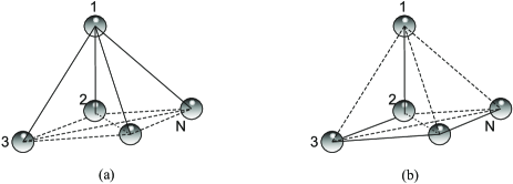
Figure 1: All $N$-qubit pure states which are SLOCC equivalent to $W$ states ($|GW\rangle$ in the text) can be determined, among arbitrary states, by the following set of bipartite marginals: (a) $\{\rho^{1K},K=2(1)N\}$; (b) $\{\rho^{K(K+1)},K=1(1)(N-1)\}$. Generally, in $|GW\rangle$ each pair of qubits is correlated (e.g., entangled), which is indicated by the edges. The set of biparite RDMs required in each case is depicted by the solid edges. We note that the figure in (a) resembles entanglement combing yangeisert09 .

IV Optimal reducibility of some other classes of states

In this section, we will generalize the result on $W$ states to two other well known classes of states namely the Dicke states $|D_{N}^{\ell}\rangle$ and the ‘$G$’ state.

IV.1 Determination of $|D_{N}^{\ell}\rangle$ from $(\ell+1)$-partite marginals

The generic Dicke states are defined by

$$|GD_{N}^{\ell}\rangle=\sum_{i}c_{i}|i\rangle,$$ (19)

where $i=i_{1}i_{2}\ldots i_{N}$ and the sum varies over all permutations of $\ell(\leq\lfloor N/2\rfloor)$ number of 1 and $N-\ell$ number of 0; $c_{i}\in\mathbb{C}$ with $\sum_{i}|c_{i}|^{2}=1$ and $c_{i}\neq 0$. The standard Dicke states (i.e., when all the coefficients are equal) are SLOCC inequivalent to each other for different $\ell$ and also inequivalent to the GHZ states dliepl09 . In our earlier work we had shown that for $\ell<\lfloor N/2\rfloor$, the class of states (19) is determined by $2\ell$-partite marginals. Also the question about its optimality was raised therein prftc2009 . It was discussed that the optimal number would lie between $[\ell+1,2\ell]$. In the spirit of our main result of the previous section, we hope that $\ell+1$ may be the optimal number. It indeed turns out to be the case. Thus we have the following general result:

Theorem 3

The class of states given by (19) is uniquely determined, among arbitrary states, by its $(\ell+1)$-partite marginals $\rho^{1P_{2}P_{3}\ldots P_{\ell+1}}_{GD},\quad P_{k}\in\{2,3,4,\ldots,N\}$.

Proof: The proof follows almost parallel to the case of $W$ states. We have to use PSD completion (third order minor) to show the uniqueness of the off-diagonals. $\blacksquare$

Note that we have used all the ($\ell+1$)-partite RDMs (${}^{N-1}C_{\ell}$ in number). Surely not all of them are required and some are redundant. But we don’t know what is the optimal number of ($\ell+1$)-partite RDMs. It follows trivially that this number can not be less than $N-\ell$.

IV.2 Optimal reducibility of the state $|G_{N}\rangle=\frac{1}{\sqrt{2}}(|W_{N}\rangle+|\bar{W}_{N}\rangle)$

Recently the correlation structure in the $N$-qubit ‘$G$’ state,

$$|G_{N}\rangle=\frac{1}{\sqrt{2}}(|W_{N}\rangle+|\bar{W}_{N}\rangle)$$ (20)

has been studied by several authors from different perspectives (for example see ausen03 ; ausen031 ; bennett11 ). The purpose of this subsection is to consider the correlation structure in $|G_{N}\rangle$ from the parts and whole point of view i.e., to determine its reducibility. This question has been raised and partially answered in ausen031 . The authors showed that for $N\geq 5$, $|G_{N}\rangle$ can be determined from $(N-1)$-partite RDMs. Here we show that the correlation is further reducible. For the sake of optimality we prove that for $N\geq 6$, the correlation in $|G_{N}\rangle$ is reducible to $(N-2)$-partite level and not beyond it.

The reducibility of three qubit $G$ state has been considered in dsrar . In fact this case follows trivially from the previous known results. It has been explicitly shown in lpw2002 that except the $|GGHZ\rangle$ and its LU equivalent states, all three-qubit pure states are determined by their bipartite RDMs. So any pure state which is SLOCC equivalent to $W$ state can be determined as it is not LU equivalent to $|GGHZ\rangle$. All other genuinely entangled states which are SLOCC but not LU equivalent to $|GGHZ\rangle$ are also determinable. Such states provide examples to a query raised in pr2009 . As an instant example, $|G_{3}\rangle$ is such a state as it is not LU but SLOCC equivalent to $|GHZ\rangle$ state (the SLOCC operator may be chosen as $\otimes^{3}_{1}A_{k}$ with $A_{k}=(-1/\sqrt[6]{3})[|0\rangle(\langle 0|+\langle 1|)+|1\rangle(\omega\langle 0|+\omega^{2}\langle 1|)]$, $\omega$ being a complex cubic root of unity).

Interestingly, however, the four qubit $G$ state is LU equivalent to the $GHZ$ state and hence cannot be determined by its RDMs!

For $N\geq 5$, relaxing the normalization, we can write

$$|G_{N}\rangle=|00\rangle|W_{N-2}\rangle+|\psi\rangle|GHZ_{N-2}\rangle+|11\rangle|\bar{W}_{N-2}\rangle$$ (21)

where $|\psi\rangle=|01\rangle+|10\rangle$. Thus any (normalized) bipartite RDM of $|G_{N}\rangle$ is given by

$$\frac{1}{2N}\left(\begin{array}[]{cccc}N-2&0&0&0\\ 0&2&2&0\\ 0&2&2&0\\ 0&0&0&N-2\\ \end{array}\right)$$

This matrix has three non-zero eigenvalues whereas any bipartite RDM of $GGHZ$ (or its LU equivalent) has only two non-zero eigenvalues. Since, unitary transformation can not change the eigenvalues, $|G_{N}\rangle$ is not LU equivalent to $|GGHZ\rangle$. Therefore, from Walck and Lyons’ result wl2009 it follows that $|G_{N}\rangle$ is uniquely determined by its (all) $(N-1)$-partite RDMs. It is amazing that six years before the general result of wl2009 , the authors of ausen031 had proven explicitly and argued that “$|G_{N}\rangle$ does not belongs to the $|GHZ\rangle$ family”.

For $N\geq 6$, we have the following stronger result:

Theorem 4

For $N\geq 6$, the $N$-qubit generic $G$ state

$$|GG_{N}\rangle=\sum_{K=1}^{N}(a_{K}|01_{K}0\ldots 0\rangle+b_{K}|10_{K}1\ldots 1\rangle)$$ (22)

(with $\sum(|a_{K}|^{2}+|b_{K}|^{2})=1$, $a_{K}b_{K}\neq 0$) is uniquely determined, among arbitrary states, by its $(N-2)$-partite RDMs, but can not be determined by lower order RDMs.

Proof: Following the proof of Theorem 1, it can be shown that $|GG_{6}\rangle$ is determined by only three RDMs $\rho^{1234},\rho^{1235},\rho^{1236}$. However, for $N\geq 7$, there is a very simple proof which is outlined below:

Since $|GG_{N}\rangle$ has no basis term containing two or three 1 (and rest zeros), comparing the coefficients of $|01_{K}0\ldots 0\rangle\langle 01_{K}0\ldots 0|$ in the RDMs, it follows that $r_{(01_{K}0\ldots 0)(01_{K}0\ldots 0)}=|a_{K}|^{2}$. Similarly, (interchanging 0 and 1) $r_{(11\ldots 10_{K}1\ldots 1)(1\ldots 10_{K}1\ldots 1)}=|b_{K}|^{2}$. Then by normalization, it follows that the mixed $\rho$ should have the same form as $|GG_{N}\rangle\langle GG_{N}|$ and share the same diagonals. Finally the off diagonals: it follows trivially (e.g., by comparing $|01_{J}0\ldots 0\rangle\langle 01_{K}0\ldots 0|$ etc.) $r_{(01_{J}0\ldots 0)(01_{K}0\ldots 0)}=a_{J}\bar{a}_{K},r_{(10_{J}1\ldots 1)(10_{K}1\ldots 1)}=b_{J}\bar{b}_{K}$ and $r_{(01_{J}0\ldots 0)(10_{K}1\ldots 1)}=a_{J}\bar{b}_{K}$. The only remaining off diagonals $r_{(01_{J}0\ldots 0)(10_{J}1\ldots 1)}$ are found to be $a_{J}\bar{b}_{J}$ by considering PSD of the principal minor consisting of rows and columns $(01_{J}0\ldots 0),(01_{K}0\ldots 0)$ and $(10_{J}1\ldots 1)$.

To prove that $|GG_{N}\rangle$ can not be determined by lower order RDMs, it is sufficient to note that it shares all $(N-3)$-partite RDMs with the following two states

$$|G^{\prime}_{N}\rangle = |W\rangle-|\bar{W}\rangle$$

$$\text{and}\quad\rho = |W\rangle\langle W|+|\bar{W}\rangle\langle\bar{W}|,$$

where the two unnormalized states are given by $|W\rangle=\sum_{K=1}^{N}a_{K}|01_{K}0\ldots 0\rangle$ and $|\bar{W}\rangle=\sum_{K=1}^{N}b_{K}|10_{K}1\ldots 1\rangle$.   $\blacksquare$

The next obvious question would be the optimal number of RDMs required. Well, it can be proved that for $N\geq 6$, only two RDMs (e.g., $\rho^{123\ldots(N-3)(N-2)},\rho^{345\ldots(N-1)N}$) are required and this is the optimal number. Here, in the last step (the PSD completion step), instead of using so many third-ordered principle minors, we may consider the fourth-ordered one consisting of the following rows and columns $(01_{J}0\ldots 0),(100\ldots 0),(101\ldots 1),(10_{k}1\ldots 1)$ and we have to use the result that the following matrix is PSD iff $a=b=c=1$:

$$\left[\begin{array}[]{cccc}1&1&a&b\\ 1&1&1&c\\ \bar{a}&1&1&1\\ \bar{b}&\bar{c}&1&1\\ \end{array}\right].$$

V Discussion and Conclusion

First of all we want to mention that though we have studied generic classes of states, except for the $W$ class ($|GW\rangle$), the term ‘generic’ means that the coefficients are arbitrary complex numbers and nothing else, whereas for the $W$-class, it includes all ‘$W$-type’ states i.e., all states which are SLOCC equivalent to the $W$ state. We note that under SLOCC, the generic Dicke state (19) transforms as

$$|GD_{N}^{(\ell)}\rangle\rightarrow\sum_{k=0}^{\ell}|GD_{N}^{(k)}\rangle.$$ (23)

Thus, under SLOCC, $|GD_{N}^{\ell}\rangle$ does not preserve its minimal form. So, it is almost impossible to check their minimal reducibility by the present technique. However, we should emphasize that this is not a shortcoming of the technique. Under SLOCC, most states change drastically and for $N\geq 4$, there are uncountable number of SLOCC inequivalent states gourwallachjmp10 . So, it is unusual to expect to explicitly express each member and then characterize the classes case by case. That is why we have considered the generic classes like this. It is also worth pointing out that each such class is also composed of several (uncountable number of) SLOCC inequivalent states. For example, using the criterion of gourwallachjmp10 , it follows immediately that the two members from the family $|GD_{4}^{2}\rangle$

$$|\psi\rangle = a|3\rangle+b|5\rangle+c|6\rangle+d|9\rangle+e|10\rangle+f|12\rangle$$

$$\text{and }|\phi\rangle = a^{\prime}|3\rangle+b^{\prime}|5\rangle+c^{\prime}|6\rangle+d^{\prime}|9\rangle+e^{\prime}|10\rangle+f^{\prime}|12\rangle$$

are SLOCC inequivalent unless $af(cd-be)=a^{\prime}f^{\prime}(c^{\prime}d^{\prime}-b^{\prime}e^{\prime})$. This also implies that all members of the family $|GD_{4}^{2}\rangle$ with $af(cd-be)\neq 0$ are SLOCC inequivalent to $|D_{4}^{2}\rangle$.

Because of the powerful result of wl2009 , it is now very easy to check whether any $N$-qubit pure state has reducible correlations or not–we just need to check whether the given state is LU equivalent to $|GGHZ\rangle$ and this question of LU equivalence has been recently solved in bkrausprl10 . However, our aim is not just to determine the reducibility, but following the spirit of the original work lpw2002 ; lw2002 , to determine how far we can reduce the correlations. This question has similar notion with separability and $K$-separability. To resolve it, we have to characterize all classes of states that can be determined by $K$-partite RDMs. Though some constraints can be derived easily, we are not yet able to address this issue. Very recently, the authors of ushaothers have applied Majorana representation to determine the reducibility of symmetric classes of states. This approach may give some insight to solve the problem.

As mentioned earlier, recently the correlation structure of $|G_{N}\rangle$ has attracted much attention. The authors of ausen031 had previously shown that the “higher order correlation is reducible to lower order ones” and thus $|G_{N}\rangle$ is weakly correlated than $|GHZ\rangle$. It follows from our result that we can lower one more level thereby making the correlation even weaker, but many much stronger than that of $W$-type state itself. It indeed is surprising that the correlation information in $|GG_{N}\rangle$ is imprinted in just two $(N-2)$-partite RDMs. A byproduct of this result is that all such states are different (LU inequivalent) from $|GGHZ\rangle$.

To conclude, we have shown that all multiqubit pure states which are SLOCC equivalent to the $N$-qubit $W$ state, are uniquely determined by their bipartite marginals. So, from the parts and whole perspective, we can say that these states contain information essentially at the bipartite level. Moreover, only ($N$-1) number of bipartite RDMs having one party common to all, are required and this number is optimal. Entanglement (by construction of any measure) is always preserved under LU but in general not under SLOCC. The same holds for (ir)reducibility in the case of $GHZ$ (and so for generic) states. However, on the contrary, for the $W$ states, it is rather surprising that reducibility is preserved under SLOCC. Prior to this work, even the reducibility of all LU equivalent $W$ states was not known. We hope our results will help to understand and explore further the correlation structure of W-type states.

*

Appendix A Proof of Theorem 2

As usual, let an $N$-qubit (generically mixed) state $\rho_{M}$, as given by Eq. (9) be such that $\rho^{K(K+1)}_{M}=\rho^{K(K+1)}_{GW}\quad\forall K=1(1)(N-1)$. We will show that $\rho_{M}=|GW\rangle\langle GW|$.

First we note that no basis of ${\rho}_{M}$ can have two consecutive 1 (means $r_{(i_{1}i_{2}\ldots i_{K-1}1_{K}1_{K+1}i_{K+2}\ldots i_{N})(j_{1}j_{2}\ldots j_{N})}=0$). Next we will show that no basis of $\rho_{M}$ can have the sequence 101 i.e. $r_{(i_{1}\ldots 1_{K}0_{K+1}1_{K+2}\ldots i_{N})(j_{1}j_{2}\ldots j_{N})}=0$. For simplicity, let us first take $K=1$ and the other cases will follow similarly. So, comparing the diagonal elements $|01\rangle\langle 01|$, $|10\rangle\langle 10|$ and the off-diagonal elements $|01\rangle\langle 10|$ from $\rho^{12}_{M}$ and $\rho^{12}_{GW}$ we have (keeping in mind that no basis can have two consecutive 1)

$$\sum_{i_{4},i_{5},\ldots,i_{N}=0}^{1}r_{(010i_{4}i_{5}\ldots i_{N})(010i_{4}i_{5}\ldots i_{N})} = |c_{2}|^{2}$$ (24a)

$$\sum_{i_{3},i_{4},\ldots,i_{N}=0}^{1}r_{(10i_{3}i_{4}\ldots i_{N})(10i_{3}i_{4}\ldots i_{N})} = |c_{1}|^{2}$$ (24b)

$$\sum_{i_{4},i_{5},\ldots,i_{N}=0}^{1}r_{(010i_{4}i_{5}\ldots i_{N})(100i_{4}i_{5}\ldots i_{N})} = c_{2}\bar{c}_{1}$$ (24c)

Considering absolute values in (24c), we have

$$\sum_{i_{4},i_{5},\ldots,i_{N}=0}^{1}|r_{(010i_{4}i_{5}\ldots i_{N})(100i_{4}i_{5}\ldots i_{N})}|\geq|c_{2}||c_{1}|$$ (25)

By the PSD property (iii), $|r_{(010i_{4}i_{5}\ldots i_{N})(100i_{4}i_{5}\ldots i_{N})}|\leq\sqrt{r_{(010i_{4}i_{5}\ldots i_{N})(010i_{4}i_{5}\ldots i_{N})}r_{(100i_{4}i_{5}\ldots i_{N})(100i_{4}i_{5}\ldots i_{N})}}$. So summing up (each sum varies over $i_{4},i_{5},\ldots,i_{N}=0$ to 1),

$$\sum|r_{(010i_{4}\ldots i_{N})(100i_{4}\ldots i_{N})}| \leq \sum\sqrt{r_{(010i_{4}\ldots i_{N})(010i_{4}\ldots i_{N})}r_{(100i_{4}\ldots i_{N})(100i_{4}\ldots i_{N})}}$$ (26a)

$$\leq \sqrt{(\sum r_{(010i_{4}\ldots i_{N})(010i_{4}\ldots i_{N})})(\sum r_{(100i_{4}\ldots i_{N})(100i_{4}\ldots i_{N})})}$$ (26b)

$$\leq |c_{2}||c_{1}|$$ (26c)

where in (26b) we have used Schwartz inequality and in (26c), we have used (24a) and (24b). It follows from (25) and (26c) that all inequalities in (25) and (A.3) should be equalities. For equality in (26c) we must have

$$\sum_{i_{4},\ldots,i_{N}=0}^{1}r_{(100i_{4}\ldots i_{N})(100i_{4}\ldots i_{N})}=|c_{1}|^{2}$$ (27)

which together with (24b) implies that $r_{(101i_{4}i_{5}\ldots i_{N})(101i_{4}i_{5}\ldots i_{N})}=0$. Comparing $\rho^{K(K+1)}_{M}$ and $\rho^{K(K+1)}_{GW}$, in a similar way we can prove that no basis of $\rho_{M}$ can contain the sequence $101$ i.e.,

$$r_{(i_{1}i_{2}\ldots i_{K-1}1_{K}0_{K+1}1_{K+2}i_{K+3}\ldots i_{N})(j_{1}j_{2}\ldots j_{N})}=0$$ (28)

Thus it follows immediately that (24c) would reduce to

$$\sum_{i_{5},i_{6},\ldots,i_{N}=0}^{1}r_{(0100i_{5}\ldots i_{N})(1000i_{5}\ldots i_{N})}=c_{2}\bar{c}_{1}$$ (29)

as well as $r_{(1001i_{5}\ldots i_{N})(j_{1}j_{2}\ldots j_{N})}=0$. Similarly, it follows that $i_{5}=0$, $i_{6}=0$ by considering $\rho^{23}$, $\rho^{34}$ and so on. For an illustration, the iterations go like:

$$\rho^{23}:~{}\sum_{i_{6},\ldots,i_{N}=0}^{1}r_{(00100i_{6}\ldots i_{N})(01000i_{6}\ldots i_{N})} = c_{3}\bar{c}_{2}$$

$$\rho^{34}:~{}\sum_{i_{7},\ldots,i_{N}=0}^{1}r_{(000100i_{7}\ldots i_{N})(001000i_{7}\ldots i_{N})} = c_{4}\bar{c}_{3}$$

and so on. The iteration stops at $\rho^{(N-1)N}$ and we will have

$$r_{(001_{K}00\ldots 0)(001_{K}00\ldots 0)} = |c_{K}|^{2}$$

$$r_{(00_{K}1_{K+1}00\ldots 0)(01_{K}0_{K+1}0\ldots 0)} = c_{K+1}\bar{c}_{K}$$ (30)

Then by normalization, $r_{(00\ldots 0)(00\ldots 0)}=|c_{0}|^{2}$. Finally, the off diagonal elements $r_{(001_{J}0\ldots 0)(01_{K}0\ldots 0)}$ are found to be $c_{J}\bar{c}_{K}$ by the repeated applications of the third-ordered PSD completion. $\blacksquare$

References

- (1) W. Dür, G. Vidal and J. I. Cirac, Phys Rev. A 62, 062314 (2000).
- (2) N. Linden, S. Popescu and W. K. Wootters, Phys. Rev. Lett. 89, 207901 (2002).
- (3) N. Linden and W. K. Wootters, Phys. Rev. Lett. 89, 277906 (2002); A. Higuchi, A. Sudbery and J. Szulc, Phys. Rev. Lett. 90, 107902 (2003); L. Diósi, Phys. Rev. A 70, 010302 (2004); Y. Feng, R. Duan and M. Ying, Quant. Inf. Comp. 9, 0997 (2009).
- (4) N. S. Jones and N. Linden, Phys. Rev. A 71 012324 (2005).
- (5) S. N. Walck and D. W. Lyons, Phys. Rev. Lett. 100, 050501 (2008); Phys. Rev. A 79, 032326 (2009).
- (6) D. L. Zhou, Phys. Rev. Lett. 101, 180505 (2008); Phys. Rev. A 80, 022113 (2009).
- (7) D. Yang and J. Eisert, Phys. Rev. Lett. 103, 220501 (2009).
- (8) P. Parashar and S. Rana, Phys. Rev. A 80, 012319 (2009).
- (9) P. Parashar and S. Rana, J. Phys. A: Math. Theor. 42, 462003 (2009).
- (10) M. A. Nielsen, Phys. Rev. Lett. 83, 436 (1999).
- (11) K. Uyanik and S. Turgut, Phys. Rev. A 81 032306 (2010).
- (12) L. Chen, E. Chitambar, R. Duan, Z. Ji and A. Winter, Phys. Rev. Lett. 105, 200501 (2010); L. Chen and M. Hayashi, Phys. Rev. A 83, 022331 (2011).
-
(13)
P. Agrawal and A. Pati, Phys. Rev. A 74, 062320 (2006);
L. Li and D. Qiu, J. Phys. A: Math. Theor. 40 10871 (2007); Z. H. Peng, J. Zou and X. J. Liu, Eur. Phys. J. D 58, 403 (2010). - (14) S. Kintas and S. Turgut, J. Math. Phys. 51, 092202 (2010).
- (15) See e.g., R. A. Horn and C. R. Johnson, Matrix analysis, published by Cambridge University Press, USA, 1985.
- (16) D. Li, X. Li, H. Huang and X. Li, EPL 87, 20006 (2009).
- (17) A. Sen(De), U. Sen, M. Wieśniak, D. Kaszlikowski and M. Żukowski, Phys. Rev. A 68, 062306 (2003); D. Kaszlikowski, A. Sen(De), U. Sen, V. Vedral and A. Winter, Phys. Rev. Lett. 101, 070502 (2008).
- (18) A. Sen(De), U. Sen and M. Żukowski, Phys. Rev. A 68, 032309 (2003).
- (19) C. H. Bennett, A. Grudka, M. Horodecki, P. Horodecki and R. Horodecki, Phys. Rev. A 83, 012312 (2011).
- (20) A. R. Usha Devi, Sudha and A. K. Rajagopal, Interconvertibility and irreducibility of permutation symmetric three qubit pure states, arXive:1002.2820 [quant-ph].
- (21) G. Gour and N. R. Wallach, J. Math. Phys. 51, 112201 (2010).
- (22) B. Kraus, Phys. Rev. Lett. 104, 020504 (2010).
- (23) A. R. Usha Devi, Sudha and A. K. Rajagopal, arXiv:1003.2450; Quantum Inf Process, DOI 10.1007/s11128-011-0280-8.