Counter–rotating stellar discs around a massive black hole: self–consistent, time–dependent dynamics

Abstract

We formulate the collisionless Boltzmann equation (CBE) for dense star clusters that lie within the radius of influence of a massive black hole in galactic nuclei. Our approach to these nearly Keplerian systems follows that of Sridhar and Touma (1999): Delaunay canonical variables are used to describe stellar orbits and we average over the fast Keplerian orbital phases. The stellar distribution function (DF) evolves on the longer time scale of precessional motions, whose dynamics is governed by a Hamiltonian, given by the orbit–averaged self–gravitational potential of the cluster. We specialize to razor–thin, planar discs and consider two counter–rotating (“$\pm$”) populations of stars. To describe discs of small eccentricities, we expand the $\pm$ Hamiltonian to fourth order in the eccentricities, with coefficients that depend self–consistently on the $\pm$ DFs. We construct approximate $\pm$ dynamical invariants and use Jeans’ theorem to construct time–dependent $\pm$ DFs, which are completely described by their centroid coordinates and shape matrices. When the centroid eccentricities are larger than the dispersion in eccentricities, the $\pm$ centroids obey a set of 4 autonomous equations ordinary differential equations. We show that these can be cast as a two–degree of freedom Hamiltonian system which is nonlinear, yet integrable. We study the linear instability of initially circular discs and derive a criterion for the counter–rotating instability. We then explore the rich nonlinear dynamics of counter–rotating discs, with focus on the variety of steadily precessing eccentric configurations that are allowed. The stability and properties of these configurations are studied as functions of parameters such as the disc mass ratios and angular momentum.

1 Introduction

Galactic nuclei have massive black holes and dense clusters of stars, whose structural and kinematic properties appear to be correlated with global galaxy properties (Gebhardt et al., 1996; Ferrarese & Merritt, 2000; Gebhardt et al., 2000). These correlations are probably the relics of the formation and evolution of the galaxy and its central black hole (Richstone et al., 1998; Hopkins & Quataert, 2011). The dynamics of star clusters around massive black holes involves physical processes under extreme conditions, because of the high stellar densities, large velocities and short time scales (Alexander, 2005; Merritt, 2006). For a star cluster with 1–dimensional velocity dispersion $\sigma$, and black hole of mass $M_{\bullet}$, the radius of influence of the black hole is traditionally defined as $r_{\rm h}=G\mbox{$M_{\bullet}$}/\sigma^{2}\,$. Within the radius of influence, i.e. for $r<r_{\rm h}$, the dynamics of stars is dominated by the gravitational attraction of the black hole. When general relativistic effects are weak enough, the orbital dynamics is a perturbation of the Kepler problem. Sridhar & Touma (1999) argued that the semi–major axis of stellar orbits would be a secularly conserved quantity, and that this greater integrability would facilitate the existence of asymmetric stellar distributions. The secular dynamical evolution of nearly Keplerian systems such as stellar clusters surrounding black holes in galactic nuclei, cometary clouds or planetesimal discs were studied by Touma et al. (2009).

For most galaxies, it is difficult to observe details of the stellar distribution for $r<r_{\rm h}\,$. Therefore, observations of the nuclear regions of our Galaxy and M31 assume special importance, because these are the nearest large, normal galaxies for which it is possible to get a great deal of photometric, kinematic and spectral information about the stars. There is evidence for a black hole of mass $\sim 4\times 10^{6}\,M_{\odot}$ at the Galactic center, with dense clusters of stars orbiting it (Genzel et al., 2010). Among these, there is a population of about 200 young stars (Paumard et al., 2006), about half which probably belong to a rotating disc which is highly warped (Levin & Beloborodov, 2003; Lu et al., 2006, 2009). The remaining young stars appear to be members of a counter–rotating population which is thicker than and inclined to the warped disc (Genzel et al., 2003; Paumard et al., 2006; Bartko et al., 2009, 2010). The nucleus of M31 has a lopsided double–peaked distribution of stars orbiting a black hole of mass $\sim 10^{8}\,M_{\odot}$, with the brighter peak off–centered, and the fainter one centered close to the black hole (Light et al., 1974; Lauer et al., 1993, 1998; Kormendy & Bender, 1999). Tremaine (1995) proposed that the off–centered peak marks the location in a stellar disc corresponding to the aligned apoapsides of several eccentric stellar orbits. Following this proposal, more detailed stellar dynamical models of the eccentric disc have been proposed (Bacon et al., 2001; Salow & Statler, 2001; Sambhus & Sridhar, 2002; Peiris & Tremaine, 2003; Bender et al., 2005). It is a very interesting fact that for both galaxies, these extraordinary stellar dynamical structures have $r<r_{\rm h}$.

An alternative and useful way of seeing the significance of the radius of influence is this: a self–gravitating star cluster that lies within $r_{\rm h}$ has mass $M<\mbox{$M_{\bullet}$}$. The orbit of a star may be thought of as a slowly evolving Keplerian ellipse of fixed semi–major axis (with the central mass at one focus), whose dynamics is governed by a Hamiltonian which is the orbit–averaged gravitational potential due to the star cluster (Sridhar & Touma, 1999). This slow secular evolution time scale is larger than the typical Keplerian orbital time by the large factor $(\mbox{$M_{\bullet}$}/M)\,$. Slow modes of Keplerian discs were first explored by Sridhar et al. (1999); Tremaine (2001). Orbital dynamics has been analyzed and classified for the cases of non-axisymmetric planar (Sridhar & Touma, 1999), and triaxial cluster potentials (Merritt & Valluri, 1999; Sambhus & Sridhar, 2000; Poon & Merritt, 2001; Merritt & Vasiliev, 2011). One purpose of classifying stellar orbits is to be able to construct stellar distribution functions (DFs) that can reproduce the photometry and kinematics of stars around massive black holes in galactic nuclei. When the time scales under consideration are smaller than the relaxation times, the DF obeys the collisionless Boltzmann equation (CBE); see Binney & Tremaine (2008). In this paper we begin with a formulation of the CBE for the self–consistent, slow secular dynamics of star clusters within the radius of influence of massive black holes.

The warped discs at the Galactic center are mutually counter–rotating. The stellar dynamical model of Sambhus & Sridhar (2002) for the lopsided stellar disc in the nucleus of M31 included a few percent of the stars on counter–rotating orbits. Here, it was proposed that the lopsidedness of the nuclear disc of M31 could have been excited by the counter–rotating instability, due to the accretion of a globular cluster that spiraled in due to dynamical friction. This proposal was motivated by the work of Touma (2002), which suggested that even a small fraction of mass in counter–rotating orbits could excite a linear lopsided instability. Touma et al. (2009) examine a secularly unstable system of counterrotating discs, and follow the unfolding and saturation of the instability into a global, uniformly precessing, lopsided ($m=1$) mode. Counter–rotating streams of matter in a self–gravitating disc are known to be unstable to lopsided modes (Zang & Hohl, 1978; Araki, 1987; Sawamura, 1988; Merritt & Stiavelli, 1990; Palmer & Papaloizou, 1990; Sellwood & Merritt, 1994; Lovelace et al., 1997; Sridhar & Saini, 2010). Mass accretion in galactic nuclei will be such that the sense of rotation of infalling material will be uncorrelated with the rotation of pre–existing material surrounding the central black hole. In other words, in the course of the evolution of a galaxy, having counter–rotating systems in its nucleus is probably generic.

The main goal of this paper is to formulate and analyze the time–dependent dynamics of counter–rotating stellar discs, which lie within the radius of influence of the black hole. In § 2 we discuss the slow dynamics of nearly Keplerian star clusters by using the Delaunay action–angle variables, and average over the fast orbital phase. We present the CBE governing the collisionless evolution of the stellar DF. The self–consistent Hamiltonian is the orbit–averaged gravitational potential due to the star cluster, where softened gravity is used. The CBE is then formulated for razor–thin, planar discs, where the phase space is seen to be topologically equivalent to a 2–sphere. In § 3 we consider counter–rotating (“$\pm$”) discs with fixed semi–major axes. Here, it proves convenient to write separate CBEs for the $\pm$ DFs in the $\pm$ phase spaces. We consider discs of small eccentricities, and introduce ”cartesian-type” canonical variables. The ring–ring interaction potential is expanded to 4th order in the eccentricities for discs with the same semi–major axes, using results from Mrouéh & Touma (2011) which are elaborated upon in Appendix A. Using this, the $\pm$ Hamiltonians are expressed in terms of the $\pm$ DFs with coefficients that depend on both $\pm$ DFs. In § 4 we construct time–dependent DFs for the $\pm$ discs. The method used is to first seek approximate dynamical invariants for the time–dependent dynamics of the gravitationally coupled $\pm$ discs, and then use Jeans’ theorem to construct time–dependent DFs. The isocontours of the DFs are ellipses centered on moving origins in the $\pm$ phase spaces. The coordinates of the centers (referred to as “centroids”) contain information about the mean eccentricities and periapse orientations of the $\pm$ DFs. Information about the dispersions of eccentricities and periapse orientations is contained in the positive–definite $2\times 2$ “shape matrices” which describe the elliptical isocontours. When the centroid eccentricities are larger than the dispersion in eccentricities, the centroid dynamics is independent of the shape dynamics; however, the shape dynamics is driven by the centroid dynamics. In § 5 we show that the coupled dynamics of the $\pm$ centroids is a two–degree of freedom Hamiltonian system which is nonlinear, yet integrable. We then study the linear instability of initially circular discs and derive a criterion for the instability. The rest of the section is an exploration of the rich nonlinear dynamics of counter–rotating discs, with focus on the variety of steadily precessing eccentric configurations that are allowed. The stability and properties of these configurations are studied as functions of parameters such as the disc mass ratios and angular momentum. Summary and conclusions are offered in § 6.

2 Collisionless evolution of nearly Keplerian stellar systems

We consider a stellar system around a central object of mass $M_{\bullet}$ . Over times shorter than the relaxation times, the system is effectively collisionless. Then the stellar system may be thought of as composed of an infinite number of stars, each of infinitesimal mass, with total mass in stars equal to $M$. Stellar orbits are governed by the Newtonian gravity of the central mass, as well as the mean–field gravitational potential of all the stars. When $(M/\mbox{$M_{\bullet}$})\ll 1$, it is useful to regard the dynamics as a perturbation of the Kepler problem. Thus the orbit of a star may be thought of as a slowly evolving Keplerian ellipse of fixed semi–major axis, with the central mass at one focus. This slow secular evolution time scale is larger than the typical Keplerian orbital time by the large factor $(\mbox{$M_{\bullet}$}/M)\,$.

Each star is a moving point–like object in the $6$–dimensional phase space, $\left(\mbox{\boldmath$r$},\mbox{\boldmath$v$}\right)$, where $r$ is its position with respect to the central mass, and $v$ is its velocity. Since the dynamics of a star is nearly Keplerian, it is useful to employ the Delaunay variables, which are action–angle variables for the Kepler problem. The Delaunay variables, $\{I,L,L_{z}\,;\,w,g,h\}$, are a set of action and angle variables for the Kepler problem (Sridhar & Touma, 1999; Binney & Tremaine, 2008). The three actions are: $I\,=\,\sqrt{G\mbox{$M_{\bullet}$}a}\,$ where $a$ is the semi–major axis; $L$, which is the magnitude of the orbital angular momentum; and $L_{z}$, which is the $z$–component of the orbital angular momentum. The angles conjugate to them are, respectively: $w$, the orbital phase; $g$, the angle to periapse from the ascending node; and $h$, the longitude of the ascending node.

In the absence of self–gravity, the motion of the star is purely Keplerian: the orbital phase $w$ advances steadily at a rate equal to the Keplerian orbital frequency, whereas the other five Delaunay variables are constant in time. However, self–gravity contributes to a slow variation of the Delaunay variables. Let $\widetilde{H}$ be the total gravitational potential seen by a star, averaged over the Keplerian orbital phase of the concerned star. Then $\widetilde{H}\,=\,\widetilde{H}(I,L,L_{z},g,h,t)$, where we have allowed for a slow time dependence. Since $\widetilde{H}$ is — by definition — independent of $w$, the conjugate momentum, $I$, is a conserved quantity; the star’s orbit can be imagined to be a slowly deforming “Gaussian ring” of fixed semi–major axis, with the central mass stationary at one focus. The slow secular evolution of the other Delaunay variables is given by

$$\frac{\mbox{${\mathrm{d}}$}L}{\mbox{${\mathrm{d}}$}t}\;=\;-\,\frac{\mbox{$\partial$}\widetilde{H}}{\mbox{$\partial$}g}\,,\qquad\frac{\mbox{${\mathrm{d}}$}g}{\mbox{${\mathrm{d}}$}t}\;=\;\frac{\mbox{$\partial$}\widetilde{H}}{\mbox{$\partial$}L}\,;\qquad\frac{\mbox{${\mathrm{d}}$}L_{z}}{\mbox{${\mathrm{d}}$}t}\;=\;-\,\frac{\mbox{$\partial$}\widetilde{H}}{\mbox{$\partial$}h}\,,\qquad\frac{\mbox{${\mathrm{d}}$}h}{\mbox{${\mathrm{d}}$}t}\;=\;\frac{\mbox{$\partial$}\widetilde{H}}{\mbox{$\partial$}L_{z}}\,.$$ (1)

Let the stellar system be described by a distribution function (DF), $f(a,L,L_{z},g,h,t)$, where $f\,\mbox{${\mathrm{d}}$}a\,\mbox{${\mathrm{d}}$}L\,\mbox{${\mathrm{d}}$}L_{z}\,\mbox{${\mathrm{d}}$}g\,\mbox{${\mathrm{d}}$}h$ is the mass in the element $\left(\mbox{${\mathrm{d}}$}a\,\mbox{${\mathrm{d}}$}L\,\mbox{${\mathrm{d}}$}L_{z}\,\mbox{${\mathrm{d}}$}g\,\mbox{${\mathrm{d}}$}h\right)$. The collisionless Boltzmann equation (CBE) which describes the time evolution of the DF is

$$\frac{\mbox{${\mathrm{d}}$}f}{\mbox{${\mathrm{d}}$}t}\;\equiv\;\frac{\partial f}{\partial t}+\left[f,\widetilde{H}\right]\;=\;0\,,$$ (2)

where

$$\left[f,\widetilde{H}\right]\;=\;\frac{\partial f}{\partial g}\,\frac{\partial\widetilde{H}}{\partial L}\;-\;\frac{\partial f}{\partial L}\,\frac{\partial\widetilde{H}}{\partial g}\;+\;\frac{\partial f}{\partial h}\,\frac{\partial\widetilde{H}}{\partial L_{z}}\;-\;\frac{\partial f}{\partial L_{z}}\,\frac{\partial\widetilde{H}}{\partial h}\,,$$ (3)

is the Poisson Bracket between $f$ and $\widetilde{H}$, defined in the $(L,L_{z},g,h)$ phase space. The Hamiltonian is

$$\widetilde{H}\;=\;\Phi_{\rm ext}(a,L,L_{z},g,h,t) - G\int\,\mbox{${\mathrm{d}}$}a^{\prime}\,\mbox{${\mathrm{d}}$}L^{\prime}\,\mbox{${\mathrm{d}}$}L^{\prime}_{z}\,\mbox{${\mathrm{d}}$}g^{\prime}\,\mbox{${\mathrm{d}}$}h^{\prime}\;f(a^{\prime},L^{\prime},L^{\prime}_{z},g^{\prime},h^{\prime},t)\;\times$$ (4)

$$\qquad\qquad\times\;\Psi(a,L,L_{z},g,h;a^{\prime},L^{\prime},L^{\prime}_{z},g^{\prime},h^{\prime}),$$

where $\Phi_{\rm ext}$ is the gravitational potential due to an external source, averaged over the star’s Keplerian orbital phase. The second term is the self–gravitational potential of the star cluster; the quantity,

$$\Psi(a,L,L_{z},g,h;a^{\prime},L^{\prime},L^{\prime}_{z},g^{\prime},h^{\prime})\;=\;\oint\oint\,\frac{dw}{2\pi}\,\frac{dw^{\prime}}{2\pi}\,\frac{1}{\left[\,\left|{\bf r}\,-\,{\bf r^{\prime}}\right|^{2}\;+\;b^{2}\;\right]^{1/2}}\;,$$ (5)

is proportional to the mutual gravitational potential energy between two particles, each of unit mass, averaged over their Keplerian orbital phases. Note that the gravitational interaction between the stars has a softening length $b$, whereas that between the central mass and a star is through an unsoftened Keplerian potential. “Softened gravity” was introduced by Miller (1971), and used as a surrogate for velocity dispersion in a stellar disc; more recent work using softened gravity in the context of nearly Keplerian systems are Touma (2002); Touma et al. (2009). Since each star is usefully imagined to be a “Gaussian ring” in secular dynamics, we refer to $\Psi$ as the ring–ring interaction function. At each value of the semi–major axis, $a$, equations (2)—(4) provide a self–consistent description of slow secular dynamics in the $(L,L_{z},g,h)$ phase space.

2.1 The CBE for razor–thin discs

When motion is restricted to a plane, the description of secular dynamics simplifies by reduction of the phase space by two dimensions. Let this plane be chosen perpendicular to the $z$–axis. The angles, $g$ and $h$, no longer have clear independent meanings; rather it is the sum $(g+h)$ that is well–defined, and we will henceforth refer to this as the angle $g$. Its conjugate variable is the scaled action variable, $\,\ell=L_{z}/\sqrt{G\mbox{$M_{\bullet}$}a}\,$, which is equal to the $z$–component of the angular momentum divided by the angular momentum of a circular orbit of radius $a\,$: this definition makes $\ell$ a normalized quantity: $-1\leq\ell\leq 1\,$. Then

$$\frac{\mbox{${\mathrm{d}}$}g}{\mbox{${\mathrm{d}}$}t}\;=\;\frac{\partial H}{\partial\ell}\,,\qquad\quad\frac{\mbox{${\mathrm{d}}$}\ell}{\mbox{${\mathrm{d}}$}t}\;=\;-\frac{\partial H}{\partial g}\,.$$ (6)

where the Hamiltonian $H(a,\ell,g,t)\;=\;\widetilde{H}/\sqrt{G\mbox{$M_{\bullet}$}a}\,$. The DF, $f(a,\ell,g,t)$, satisfies the CBE:

$$\frac{\mbox{${\mathrm{d}}$}f}{\mbox{${\mathrm{d}}$}t}\;\equiv\;\frac{\partial f}{\partial t}+\left[f,H\right]\;=\;0\,,$$ (7)

where

$$\left[f,H\right]\;=\;\frac{\partial f}{\partial g}\,\frac{\partial H}{\partial\ell}\;-\;\frac{\partial f}{\partial\ell}\,\frac{\partial H}{\partial g}\,$$ (8)

is the Poisson Bracket between $f$ and $H$, defined in the $(\ell,g)$ phase space. $H$ is determined self–consistently through

$$H\;=\;\Phi_{\rm ext}(a,\ell,g,t)\;-\;\frac{G}{\sqrt{G\mbox{$M_{\bullet}$}a}}\int\mbox{${\mathrm{d}}$}a^{\prime}\mbox{${\mathrm{d}}$}\ell^{\prime}\mbox{${\mathrm{d}}$}g^{\prime}\,f(a^{\prime},\ell^{\prime},g^{\prime},t)\,\Psi(a,\ell,g;a^{\prime},\ell^{\prime},g^{\prime}).$$ (9)

Note that the kinetic energy and the Kepler part of the potential energy have been omitted because their sum which is equal to $-G\mbox{$M_{\bullet}$}/2a$ is a constant. The $(\ell,g)$ phase space is, topologically speaking, a 2–dimensional sphere, with $\ell$ equal to the cosine of the colatitude and $g$ equal to the azimuthal angle: $\ell=\pm 1$ are located at the north and south poles respectively, whereas $\ell=0$ corresponds to the equator. For each value of the semi–major axis, $a$, equations (7)—(9) provide a self–consistent description of slow secular dynamics on this 2–sphere.

3 Counter–rotating discs: formalism for small eccentricities

In our study of counter–rotating discs we restrict attention to isolated ($\Phi_{\rm ext}=0$) planar, razor–thin discs around a central mass. We also assume that all stars in a disc have the same semi–major axis: the $+$ disc has stars with semi–major axis equal to $a_{+}$ and $-$ disc has stars with semi–major axis equal to $a_{-}$. Thus we choose the DF to be of the form,

$$f(a,\ell,g,t)\;=\;\delta(a-a_{+})\,f^{+}(\ell,g,t)\;\;+\;\;\delta(a-a_{-})\,f^{-}(\ell,g,t),$$ (10)

where the $\delta$–functions fix the semi–major axes of the two populations, which are now described by two different DFs, $f^{+}$ and $f^{-}$. These DFs obey separate CBEs:

$$\frac{\partial f^{+}}{\partial t}\;+\;\left[f^{+},H^{+}\right]\;=\;0\,;\qquad\quad\frac{\partial f^{-}}{\partial t}\;+\;\left[f^{-},H^{-}\right]\;=\;0\,,$$ (11)

where $H^{\pm}$ are the Hamiltonians acting on the $\pm$ populations, respectively. Each of $H^{+}$ and $H^{-}$ depends on both $f^{+}$ and $f^{-}$, leading to coupled dynamics of the $\pm$ populations. In fact,

$$H^{+}(\ell,g,t) = -\,\frac{G}{\sqrt{G\mbox{$M_{\bullet}$}a_{+}}}\int\mbox{${\mathrm{d}}$}\ell^{\prime}\mbox{${\mathrm{d}}$}g^{\prime}\,f^{+}(\ell^{\prime},g^{\prime},t)\,\Psi(a_{+},\ell,g;a_{+},\ell^{\prime},g^{\prime})\;\;-\;$$ (12)

$$-\,\frac{G}{\sqrt{G\mbox{$M_{\bullet}$}a_{+}}}\int\mbox{${\mathrm{d}}$}\ell^{\prime}\mbox{${\mathrm{d}}$}g^{\prime}\,f^{-}(\ell^{\prime},g^{\prime},t)\,\Psi(a_{+},\ell,g;a_{-},\ell^{\prime},g^{\prime}),$$

and

$$H^{-}(\ell,g,t) = -\,\frac{G}{\sqrt{G\mbox{$M_{\bullet}$}a_{-}}}\int\mbox{${\mathrm{d}}$}\ell^{\prime}\mbox{${\mathrm{d}}$}g^{\prime}\,f^{-}(\ell^{\prime},g^{\prime},t)\,\Psi(a_{-},\ell,g;a_{-},\ell^{\prime},g^{\prime})\;\;-\;$$ (13)

$$-\,\frac{G}{\sqrt{G\mbox{$M_{\bullet}$}a_{-}}}\int\mbox{${\mathrm{d}}$}\ell^{\prime}\mbox{${\mathrm{d}}$}g^{\prime}\,f^{+}(\ell^{\prime},g^{\prime},t)\,\Psi(a_{-},\ell,g;a_{+},\ell^{\prime},g^{\prime})\,.$$

We now specialize to counter–rotating discs of small eccentricities: let $f^{+}$ be the DF for a prograde population, which is concentrated around $\ell=+1$, and $f^{-}$ be the DF for a retrograde DF which is concentrated around $\ell=-1$. We are interested in recovering a truncated model for the collective dynamics of these coupled populations. We recall that the $(\ell,g)$ phase space is a 2–sphere, with $\ell$ equal to the cosine of the colatitude and $g$ equal to the azimuthal angle. The prograde and retrograde populations we consider are concentrated at the north and south poles, respectively. So it is convenient to use two different coordinate patches to describe the two populations. Thus we choose separate prograde and retrograde canonical variables

$$I_{+} = 1-\ell\,,\qquad\quad\theta_{+}\;=\;-g\;;$$

$$I_{-} = 1+\ell\,,\qquad\quad\theta_{-}=g\,.$$ (14)

We will also find it convenient to use the “cartesian counterparts” of the $(I,\theta)$ variables. These are defined by

$$x_{+} = \sqrt{2I_{+}}\,\sin\theta_{+}\;=\;-\sqrt{2(1-\ell)}\,\sin g\,,$$

$$y_{+} = \sqrt{2I_{+}}\,\cos\theta_{+}\;=\;\sqrt{2(1-\ell)}\,\cos g\,;$$ (15)

$$x_{-} = \sqrt{2I_{-}}\,\sin\theta_{-}\;=\;\sqrt{2(1+\ell)}\,\sin g\,,$$

$$y_{-} = \sqrt{2I_{-}}\,\cos\theta_{-}\;=\;\sqrt{2(1+\ell)}\,\cos g.$$ (16)

Here $x_{\pm}$ are new coordinates, and $y_{\pm}$ are new momenta for the $\pm$ populations. The transformations from old to new variable are of course canonical and can be simply recovered with the help of the generating function $S(x_{\pm},{\theta}_{\pm})=(x_{\pm}^{2}/2)\cot{\theta}_{\pm}$.

Before we plunge into a series of approximations that will yield the reduced dynamics, we further simplify the model disc, by further specializing to $\pm$ populations with the same semi-major axes:

$$a_{+}\;=\;a_{-}\;=\;a_{0}\,.$$ (17)

The principal advantage of this restriction is that the ring–ring interaction function, $\Psi$, can be described by fewer constants, allowing us to develop the theory with less clutter. However it may miss describing new phenomena when $a_{+}\neq a_{-}$. We reiterate:

• We will study the planar secular dynamics of two counter–rotating stellar discs of small eccentricities, around a central massive object.

• All the stars are assumed to have the same (conserved) semi–major axis.

• Each star has a single degree of a freedom, namely the freedom to adjust its periapse orientation and conjugate eccentricity in response to collective (smooth) gravitational potential of all the other stars.

• A star can, of course, change the sign of its orbital angular momentum and switch membership from the $+$ population to the $-$ population (or vice versa), while preserving its semi–major axis. However, this freedom is not allowed in what follows and shall be relaxed in future considerations of this problem.

3.1 Expansion of the ring–ring interaction function

To work out the Hamiltonians $H^{+}$ and $H^{-}$, we expand the ring–ring interaction function, $\Psi$, to $4^{\rm th}$ order in the eccentricities of the rings. This expansion was developed by Mrouéh & Touma (2011), and is given in the Appendix A. Let us define ${\bf e}$ and ${\bf e^{\prime}}$, the eccentricity vectors characterizing two rings:

$${\bf e}\;=\;(e\cos g\,,\,e\sin g\,)\;;\qquad\quad{\bf e^{\prime}}\;=\;(e^{\prime}\cos g^{\prime}\,,\,e^{\prime}\sin g^{\prime}\,)\,,$$ (18)

with $e=\sqrt{1-{\ell}^{2}}$ and $e^{\prime}=\sqrt{1-{\ell^{\prime}}^{2}}$. In the expansion of $\Psi$ we drop terms of the following type: (i) terms that are independent of ${\bf e}$ because these do not contribute to the dynamics of the concerned ring; (ii) terms higher that $4^{\rm th}$ order in ${\bf e},{\bf e}^{\prime}$, because this is the accuracy we aim for. Then,

$$\sqrt{\frac{G}{\mbox{$M_{\bullet}$}a_{0}}}\,\Psi\;\;=\;\;\alpha e^{2}\;+\;\beta{\bf e}\cdot{\bf e^{\prime}}\;+\;\gamma e^{2}e^{\prime 2}\;+\;\lambda\left({\bf e}\cdot{\bf e^{\prime}}\right)^{2}\;+\;\kappa\left({\bf e}\cdot{\bf e^{\prime}}\right)e^{\prime 2}\;+\;\chi e^{4}\;+\;\kappa e^{2}\left({\bf e}\cdot{\bf e^{\prime}}\right)\,,$$ (19)

where the coefficients $(\alpha,\beta,\gamma,\lambda,\kappa,\chi)$ are functions of $a_{0}$ and $b$, and are given in terms of the softened Laplace coefficients (see the Appendix A). Note that $3^{\rm rd}$ order terms are absent. Each of the ${\bf e}$ and ${\bf e^{\prime}}$ can belong to either the $+$ or $-$ population, so there are four possibilities. We first express ${\bf e}$ in terms of $\left(x_{\pm},y_{\pm}\right)$ accurate to $4^{\rm th}$ order. For the $+$ population equations (14) and (15) give:

$$e^{2} = 1-\ell^{2}\begin{array}[]{cccc}=&1\;-\;\left(1-I_{+}\right)^{2}&=&x_{+}^{2}\;+\;y_{+}^{2}\;-\;\frac{1}{4}\left(x_{+}^{2}+y_{+}^{2}\right)^{2}\end{array}$$ (21)

$$e\cos g = \sqrt{2I_{+}\left(1-\frac{I_{+}}{2}\right)}\,\cos\theta_{+}\begin{array}[]{cc}=&y_{+}\sqrt{1-\frac{1}{4}\left(x_{+}^{2}+y_{+}^{2}\right)}\end{array}$$ (23)

$$e\sin g = -\,\sqrt{2I_{+}\left(1-\frac{I_{+}}{2}\right)}\,\sin\theta_{+}\begin{array}[]{cc}=&-\,x_{+}\sqrt{1-\frac{1}{4}\left(x_{+}^{2}+y_{+}^{2}\right)}\;.\end{array}$$ (25)

Similarly, for the $-$ population, equations (14) and (16) give:

$$e\cos g = \sqrt{2I_{-}\left(1-\frac{I_{-}}{2}\right)}\,\cos\theta_{-}\begin{array}[]{cc}=&y_{-}\sqrt{1-\frac{1}{4}\left(x_{-}^{2}+y_{-}^{2}\right)}\end{array}$$ (27)

$$e\sin g = \,\sqrt{2I_{-}\left(1-\frac{I_{-}}{2}\right)}\,\sin\theta_{-}\begin{array}[]{cc}=&\,x_{-}\sqrt{1-\frac{1}{4}\left(x_{-}^{2}+y_{-}^{2}\right)}\;.\end{array}$$ (29)

To express ${\bf e^{\prime}}$ in terms of $\left(x^{\prime}_{\pm},y^{\prime}_{\pm}\right)$ we simply add the primes to the above expressions. Our next task is to obtain expressions for $\Psi(+,+^{\prime})$, $\Psi(+,-^{\prime})$, $\Psi(-,+^{\prime})$, and $\Psi(-,-^{\prime})$ to the same order. We begin with $\Psi(+,+^{\prime})$, by working out the terms involved in the $(+,+^{\prime})$ interactions. Using equation (25), we have:

$$e^{2} = x_{+}^{2}\;+\;y_{+}^{2}\;-\;\frac{1}{4}\left(x_{+}^{2}\,+\,y_{+}^{2}\right)^{2}\,,$$

$${\bf e}\cdot{\bf e^{\prime}} = \left(x_{+}x^{\prime}_{+}\,+\,y_{+}{y^{\prime}}_{+}\right)\,\sqrt{\left(1\,-\,\frac{x_{+}^{2}\,+\,y_{+}^{2}}{4}\right)\left(1-\frac{{x^{\prime}}_{+}^{2}\,+\,{y^{\prime}}_{+}^{2}}{4}\right)}$$

$$= \left(x_{+}x^{\prime}_{+}\,+\,y_{+}{y^{\prime}}_{+}\right)\left[\,1\;-\;\frac{x_{+}^{2}\,+\,y_{+}^{2}\,+\,{x^{\prime}}_{+}^{2}\,+\,{y^{\prime}}_{+}^{2}}{8}\right]\;+\;\ldots\,.$$

$$e^{2}{e^{\prime}}^{2} = \left(x_{+}^{2}\,+\,y_{+}^{2}\right)\left({x^{\prime}}_{+}^{2}\,+\,{y^{\prime}}_{+}^{2}\right)\;+\;\ldots$$

$$\left({\bf e}\cdot{\bf e^{\prime}}\right)^{2} = \left(x_{+}x^{\prime}_{+}+y_{+}{y^{\prime}}_{+}\right)^{2}\;+\;\ldots$$

$$e^{\prime 2}\,{\bf e}\cdot{\bf e^{\prime}} = \left({x^{\prime}}_{+}^{2}+{y^{\prime}}_{+}^{2}\right)\left(x_{+}x^{\prime}_{+}+y_{+}{y^{\prime}}_{+}\right)\;+\;\ldots$$

$$e^{4} = \left(x_{+}^{2}+y_{+}^{2}\right)^{2}\;+\;\ldots$$

$$e^{2}\,{\bf e}\cdot{\bf e^{\prime}} = \left({x}_{+}^{2}+{y}_{+}^{2}\right)\left(x_{+}x^{\prime}_{+}+y_{+}{y^{\prime}}_{+}\right)\;+\;\ldots\;.$$ (30)

Then, substituting equations (30) in (19), the interaction function between two prograde rings reduces to:

$$\sqrt{\frac{G}{\mbox{$M_{\bullet}$}a_{0}}}\,{\Psi}(+,+^{\prime}) = \left[\alpha+\gamma\left({x^{\prime}}_{+}^{2}+{y^{\prime}}_{+}^{2}\right)+\lambda{x^{\prime}}_{+}^{2}\right]\,x_{+}^{2}$$ (31)

$$+ \left[\alpha+\gamma\left({x^{\prime}}_{+}^{2}+{y^{\prime}}_{+}^{2}\right)+\lambda{y^{\prime}}_{+}^{2}\right]\,y_{+}^{2}\;+\;[2\lambda x^{\prime}_{+}{y^{\prime}}_{+}]\,x_{+}y_{+}$$

$$+ \left[\beta{x^{\prime}}_{+}+\left(\kappa-\frac{\beta}{8}\right){x^{\prime}}_{+}\left({{x^{\prime}}}_{+}^{2}+{y^{\prime}}_{+}^{2}\right)\right]\,x_{+}$$

$$+ \left[\beta{y^{\prime}}_{+}+\left(\kappa-\frac{\beta}{8}\right){y^{\prime}}_{+}\left({x^{\prime}}_{+}^{2}+{y^{\prime}}_{+}^{2}\right)\right]\,y_{+}$$

$$+ \left[\left(\kappa-\frac{\beta}{8}\right){x^{\prime}}_{+}\right]\,x_{+}\left(x_{+}^{2}+y_{+}^{2}\right)$$

$$+ \left[\left(\kappa-\frac{\beta}{8}\right){y^{\prime}}_{+}\right]\,y_{+}\left(x_{+}^{2}+y_{+}^{2}\right)\;+\;\left(\chi-\frac{\alpha}{4}\right)\,\left(x_{+}^{2}+y_{+}^{2}\right)^{2}\;,$$

where we have lumped all the dependences on primed quantities within the square brackets. Similarly, we compute quantities for the $(+,-^{\prime})$ interactions using equations (29). Then,

$$\sqrt{\frac{G}{\mbox{$M_{\bullet}$}a_{0}}}\,{\Psi}(+,-^{\prime}) = \left[\alpha+\gamma\left({x^{\prime}}_{-}^{2}+{y^{\prime}}_{-}^{2}\right)+\lambda{x^{\prime}}_{-}^{2}\right]\,x_{+}^{2}$$ (32)

$$+ \left[\alpha+\gamma\left({x^{\prime}}_{-}^{2}+{y^{\prime}}_{-}^{2}\right)+\lambda{y^{\prime}}_{-}^{2}\right]\,y_{+}^{2}\;-\;[2\lambda x^{\prime}_{-}{y^{\prime}}_{-}]\,x_{+}y_{+}$$

$$- \left[\beta{x^{\prime}}_{-}+\left(\kappa-\frac{\beta}{8}\right){x^{\prime}}_{-}\left({{x^{\prime}}}_{-}^{2}+{y^{\prime}}_{-}^{2}\right)\right]\,x_{+}$$

$$+ \left[\beta{y^{\prime}}_{-}+\left(\kappa-\frac{\beta}{8}\right){y^{\prime}}_{-}\left({x^{\prime}}_{-}^{2}+{y^{\prime}}_{-}^{2}\right)\right]\,y_{+}$$

$$- \left[\left(\kappa-\frac{\beta}{8}\right){x^{\prime}}_{-}\right]\,x_{+}\left(x_{+}^{2}+y_{+}^{2}\right)$$

$$+ \left[\left(\kappa-\frac{\beta}{8}\right){y^{\prime}}_{-}\right]\,y_{+}\left(x_{+}^{2}+y_{+}^{2}\right)\;+\;\left(\chi-\frac{\alpha}{4}\right)\,\left(x_{+}^{2}+y_{+}^{2}\right)^{2}\;.$$

3.2 Self–consistency: Hamiltonians in terms of the DFs

We can now compute $H^{+}$ by using equations (31) and (32) in (12). Then, obtaining an expression for $H^{-}$ is just a matter of switching signs: replace all the $+$ variables by the $-$ variables and vice versa. Putting together all these expansions, one finally recovers the Hamiltonians governing the prograde and retrograde populations:

$$H^{\pm} = \frac{1}{2}A_{\pm}x^{2}_{\pm}\;+\;B_{\pm}x_{\pm}y_{\pm}\;+\;\frac{1}{2}C_{\pm}y^{2}_{\pm}\;+\;D_{\pm}x_{\pm}\;+\;E_{\pm}y_{\pm}$$ (33)

$$+ F_{\pm}x_{\pm}\left(x^{2}_{\pm}\,+\,y^{2}_{\pm}\right)\;+\;G_{\pm}y_{\pm}\left(x^{2}_{\pm}\,+\,y^{2}_{\pm}\right)+K\left(x^{2}_{\pm}\,+\,y^{2}_{\pm}\right)^{2}\,,$$

where the coefficients are determined self–consistently in terms of the DFs $f^{+}$ and $f^{-}$ by,

$$A_{\pm}(t) = -\,2\int\mbox{${\mathrm{d}}$}x_{\pm}\mbox{${\mathrm{d}}$}y_{\pm}\,f^{\pm}(x_{\pm},y_{\pm},t)\left[\alpha+(\gamma+\lambda)x_{\pm}^{2}+\gamma y_{\pm}^{2}\right]$$

$$-\,2\int\mbox{${\mathrm{d}}$}x_{\mp}\mbox{${\mathrm{d}}$}y_{\mp}\,f^{\mp}(x_{\mp},y_{\mp},t)\left[\alpha+(\gamma+\lambda)x_{\mp}^{2}+\gamma y_{\mp}^{2}\right]$$

$$B_{\pm}(t) = -\,2\lambda\int\mbox{${\mathrm{d}}$}x_{\pm}\mbox{${\mathrm{d}}$}y_{\pm}\,f^{\pm}(x_{\pm},y_{\pm},t)x_{\pm}y_{\pm}\;+\;2\lambda\int\mbox{${\mathrm{d}}$}x_{\mp}\mbox{${\mathrm{d}}$}y_{\mp}f^{\mp}(x_{\mp},y_{\mp},t)x_{\mp}y_{\mp}$$

$$C_{\pm}(t) = -\,2\int\mbox{${\mathrm{d}}$}x_{\pm}\mbox{${\mathrm{d}}$}y_{\pm}\,f^{\pm}(x_{\pm},y_{\pm},t)\left[\alpha+\gamma x_{\pm}^{2}+(\gamma+\lambda)y_{\pm}^{2}\right]$$

$$-\,2\int\mbox{${\mathrm{d}}$}x_{\mp}\mbox{${\mathrm{d}}$}y_{\mp}\,f^{\mp}(x_{\mp},y_{\mp},t)\left[\alpha+\gamma x_{\mp}^{2}+(\gamma+\lambda)y_{\mp}^{2}\right]$$

$$D_{\pm}(t) = -\,\int\mbox{${\mathrm{d}}$}x_{\pm}\mbox{${\mathrm{d}}$}y_{\pm}\,f^{\pm}(x_{\pm},y_{\pm},t)\left[\beta x_{\pm}+\left(\kappa-\frac{\beta}{8}\right)x_{\pm}\left(x_{\pm}^{2}+y_{\pm}^{2}\right)\right]$$

$$+\,\int\mbox{${\mathrm{d}}$}x_{\mp}\mbox{${\mathrm{d}}$}y_{\mp}\,f^{\mp}(x_{\mp},y_{\mp},t)\left[\beta x_{\mp}+\left(\kappa-\frac{\beta}{8}\right)x_{\mp}\left(x_{\mp}^{2}+y_{\mp}^{2}\right)\right]$$

$$E_{\pm}(t) = -\,\int\mbox{${\mathrm{d}}$}x_{\pm}\mbox{${\mathrm{d}}$}y_{\pm}\,f^{\pm}(x_{\pm},y_{\pm},t)\left[\beta y_{\pm}+\left(\kappa-\frac{\beta}{8}\right)y_{\pm}\left(x_{\pm}^{2}+y_{\pm}^{2}\right)\right]$$

$$-\,\int\mbox{${\mathrm{d}}$}x_{\mp}\mbox{${\mathrm{d}}$}y_{\mp}\,f^{\mp}(x_{\mp},y_{\mp},t)\left[\beta y_{\mp}+\left(\kappa-\frac{\beta}{8}\right)y_{\mp}\left(x_{\mp}^{2}+y_{\mp}^{2}\right)\right]$$

$$F_{\pm}(t) = -\left(\kappa-\frac{\beta}{8}\right)\int\mbox{${\mathrm{d}}$}x_{\pm}\mbox{${\mathrm{d}}$}y_{\pm}\,f^{\pm}(x_{\pm},y_{\pm},t)x_{\pm}\;+\;\left(\kappa-\frac{\beta}{8}\right)\int\mbox{${\mathrm{d}}$}x_{\mp}\mbox{${\mathrm{d}}$}y_{\mp}\,f^{\mp}(x_{\mp},y_{\mp},t)x_{\mp}$$

$$G_{\pm}(t) = -\left(\kappa-\frac{\beta}{8}\right)\int\mbox{${\mathrm{d}}$}x_{\pm}\mbox{${\mathrm{d}}$}y_{\pm}\,f^{\pm}(x_{\pm},y_{\pm},t)y_{\pm}\;-\;\left(\kappa-\frac{\beta}{8}\right)\int\mbox{${\mathrm{d}}$}x_{\mp}\mbox{${\mathrm{d}}$}y_{\mp}\,f^{\mp}(x_{\mp},y_{\mp},t)y_{\mp}$$

$$K = -\left(\chi-\frac{\alpha}{4}\right)\int\mbox{${\mathrm{d}}$}x_{+}\mbox{${\mathrm{d}}$}y_{+}\,f^{+}\;-\;\left(\chi-\frac{\alpha}{4}\right)\int\mbox{${\mathrm{d}}$}x_{-}\mbox{${\mathrm{d}}$}y_{-}\,f^{-}\;=\;-\left(\chi-\frac{\alpha}{4}\right)M\,,$$ (34)

where

$$M_{\pm}\;=\;\int\mbox{${\mathrm{d}}$}x_{\pm}\mbox{${\mathrm{d}}$}y_{\pm}\,f^{\pm}(x_{\pm},y_{\pm},t)\;=\;\mbox{constant}$$ (35)

are the (constant) masses in $\pm$ populations, and $M=M_{+}+M_{-}$ is the total mass in both discs.

The coefficients $\left(A_{\pm},B_{\pm},C_{\pm},D_{\pm},E_{\pm},F_{\pm},G_{\pm}\right)$ are all, in general, functions of time, whereas $K$ is a constant proportional to the total mass in both discs. Since we have defined separate canonical variables for the $\pm$ populations, it is necessary to take care to write the CBEs of equation (11) as

$$\frac{\partial f^{+}}{\partial t}\;+\;\left[f^{+},H^{+}\right]_{+}\;=\;0\,;\qquad\quad\frac{\partial f^{-}}{\partial t}\;+\;\left[f^{-},H^{-}\right]_{-}\;=\;0\,,$$ (36)

where we have put $\pm$ subscripts on the Poisson Brackets to indicate that they are to be taken with respect to the appropriate set of canonical variables. Then the CBEs in equation (36) together with the expressions for $H^{\pm}$ given in equations (33) and (34) completely define the self–consistent evolution of the counter–rotating discs, accurate to $4^{\rm th}$ order in the eccentricities.

4 Counter–rotating discs: time–dependent DFs

In galactic dynamics, it is possible to construct many steady state solutions of the self–consistent CBE, whereas time–dependent behaviour is very difficult to understand even in the linearized limit. However, the present case of counter–rotating discs of small eccentricities around a central object turns out to be more tractable. The self–consistent dynamics described by equations (33)—(36) has implicit in it a certain approximate integrable dynamics. This remarkable circumstance allows us to construct approximate time–dependent, self–consistent DFs, and describe the evolution of the counter–rotating instability largely analytically.

4.1 An approximate dynamical invariant

In this subsection we are interested in the construction of an approximate invariant for the dynamics on a two dimensional phase space, generated by a time–dependent Hamiltonian which is similar in form to those of equations (33). We drop the $\pm$ signifiers on all quantities in the interests of reducing clutter, but will restore them in the next subsection. Hence consider the Hamiltonian

$$H(x,y,t) = \frac{1}{2}A(t)x^{2}\;+\;B(t)xy\;+\;\frac{1}{2}C(t)y^{2}\;+\;D(t)x\;+\;E(t)y$$ (37)

$$+\,F(t)x\left(x^{2}+y^{2}\right)\;+\;G(t)y\left(x^{2}+y^{2}\right)\;+\;K\left(x^{2}+y^{2}\right)^{2}\,.$$

This is a time–dependent Hamiltonian acting on the two–dimensional phase space $(x,y)$. We now seek to eliminate the linear terms in $H$ by making a canonical transformation to new coordinate and momentum, $\left({\xi}_{1},{\xi}_{2}\right)$, through a generating function

$$S(x,{\xi}_{2},t)\;=\;\left[x\,-\,X(t)\right]\left[{\xi}_{2}\,+\,Y(t)\right]\,,$$ (38)

where $X(t)$ and $Y(t)$ are some time–dependent functions, which are to be determined. Since $y=\left(\partial S/\partial x\right)$ and $\xi_{1}=\left(\partial S/\partial\xi_{2}\right)$, the transformation

$$x\;=\;{\xi}_{1}+X(t)\,;\qquad\quad y\;=\;{\xi}_{2}+Y(t)\,,$$ (39)

amounts to a time–dependent shift of the origin of phase space. The new Hamiltonian is given by

$$H_{\rm t}\left({\xi}_{1},{\xi}_{2},t\right) = H\left(x\left({\xi}_{1},{\xi}_{2}\right),y\left({\xi}_{1},{\xi}_{2}\right),t\right)\;+\;\frac{\partial S}{\partial t}$$ (40)

$$= H_{\rm lin}\;+\;H^{(0)}_{\rm t}\;+\;H^{(1)}_{\rm t}\,,$$

where $H_{\rm lin}$, $H^{(0)}_{\rm t}$ and $H^{(1)}_{\rm t}$ contain terms that are linear, quadratic, and cubic plus fourth order in $\left({\xi}_{1},{\xi}_{2}\right)$, respectively. It is straightforward to work out that

$$H_{\rm lin} = AX{\xi}_{1}\;+\;BY{\xi}_{1}\;+\;BX{\xi}_{2}\;+\;CY{\xi}_{2}\;+\;D{\xi}_{1}\;+\;E{\xi}_{2}$$ (41)

$$+ F{\xi}_{1}(X^{2}+Y^{2})\;+\;2FX(X{\xi}_{1}\;+\;Y{\xi}_{2})\;+\;G{\xi}_{2}(X^{2}+Y^{2})\;+\;2GY(X{\xi}_{1}+Y{\xi}_{2})$$

$$+ 4K[(Y^{3}+YX^{2}){\xi}_{2}+(X^{3}+XY^{2}){\xi}_{1}]\;+\;\frac{\mbox{${\mathrm{d}}$}Y}{\mbox{${\mathrm{d}}$}t}{\xi}_{1}\;-\;\frac{\mbox{${\mathrm{d}}$}X}{\mbox{${\mathrm{d}}$}t}{\xi}_{2}\,.$$

We now require that $H_{\rm lin}$ vanishes. This happens when $X(t)$ and $Y(t)$ obey the following first order ordinary differential equations (ODEs):

$$\frac{\mbox{${\mathrm{d}}$}X}{\mbox{${\mathrm{d}}$}t} = BX\;+\;CY\;+\;E\;+\;2FXY\;+\;G(X^{2}+3Y^{2})\;+\;4K(Y^{3}+YX^{2})$$

$$\frac{\mbox{${\mathrm{d}}$}Y}{\mbox{${\mathrm{d}}$}t} = -\,AX\;-\;BY\;-\;D\;-\;F(3X^{2}+Y^{2})\;-\;2GXY\;-\;4K(X^{3}+XY^{2})\,.$$ (42)

Having eliminated $H_{\rm lin}$, the remaining terms in the new Hamiltonian are $H^{(0)}_{\rm t}$ and $H^{(1)}_{\rm t}$. We require the former:

$$H_{\rm t}^{(0)}\left({\xi}_{1},{\xi}_{2},t\right)\;=\;\frac{1}{2}A_{\rm t}(t){\xi}_{1}^{2}\;+\;B_{\rm t}(t){\xi}_{1}{\xi}_{2}\;+\;\frac{1}{2}C_{\rm t}(t){\xi}_{2}^{2}\,,$$ (43)

where the new coefficients,

$$\frac{A_{\rm t}}{2} = \frac{A}{2}\;+\;3FX\;+\;GY\;+\;2K(Y^{2}+3X^{2})$$

$$B_{\rm t} = B\;+\;2FY\;+\;2GX\;+\;8KXY$$

$$\frac{C_{\rm t}}{2} = \frac{C}{2}\;+\;FX\;+\;3GY\;+\;2K(X^{2}+3Y^{2})\,,$$ (44)

are given in terms of the old coefficients and the centroid coordinates.

The homogeneous, linear and time–dependent dynamics generated by $H_{\rm t}^{0}$ preserves areas in $\left({\xi}_{1},{\xi}_{2}\right)$ space. Moreover, initial conditions given on any ellipse centered at $\xi_{1}=0$ and $\xi_{2}=0$ will, at a later time, lie on some other centered ellipse of the same area. Therefore, there must be a quadratic quantity that is preserved by the dynamics. Let us write this invariant as:

$$J\;=\;\frac{1}{2}\mbox{\boldmath$\xi$}^{\rm T}\,\mbox{\boldmath$Q$}(t)\,\mbox{\boldmath$\xi$}\;=\;\frac{1}{2}Q_{i\,j}(t){\xi}_{i}{\xi}_{j}\,,$$ (45)

where $\mbox{\boldmath$Q$}(t)$ is a time–dependent, positive definite, $2\times 2$ matrix. Because phase areas are conserved, ${\det}(\mbox{\boldmath$Q$})$ is constant. The linear dynamics generated by $H_{\rm t}^{(0)}$ can be written in matrix form as:

$$\frac{\mbox{${\mathrm{d}}$}\mbox{\boldmath$\xi$}}{\mbox{${\mathrm{d}}$}t}\;=\;\mbox{\boldmath$T$}(t)\mbox{\boldmath$\xi$}\,;\qquad\quad\mbox{\boldmath$T$}(t)\;=\;\left(\begin{array}[]{lr}B_{\rm t}&C_{\rm t}\\ -A_{\rm t}&-B_{\rm t}\end{array}\right)\,,$$ (46)

where we have introduced $\mbox{\boldmath$T$}(t)$, which is a time–dependent, traceless, $2\times 2$ matrix. If $J$, given in equation (45), is an invariant of the dynamics, we must have

$$\frac{\mbox{${\mathrm{d}}$}J}{\mbox{${\mathrm{d}}$}t}\;\equiv\;\frac{1}{2}\mbox{\boldmath$\xi$}^{\rm T}\left[\mbox{\boldmath$T$}^{\rm T}\mbox{\boldmath$Q$}\,+\,\mbox{\boldmath$Q$}\mbox{\boldmath$T$}\,+\,\frac{d\mbox{\boldmath$Q$}}{dt}\right]\mbox{\boldmath$\xi$}\;=\;0\,.$$ (47)

Therefore $\mbox{\boldmath$Q$}(t)$ must obey the matrix ODE:

$$\frac{\mbox{${\mathrm{d}}$}\mbox{\boldmath$Q$}}{\mbox{${\mathrm{d}}$}t}\;=\;-\,\mbox{\boldmath$T$}^{\rm T}\mbox{\boldmath$Q$}\;-\;\mbox{\boldmath$Q$}\,\mbox{\boldmath$T$}\,.$$ (48)

It can be verified that the equation above preserves ${\det}(\mbox{\boldmath$Q$})$.

4.2 Distribution functions

We are now ready to deal with the self–consistent dynamics of counter–rotating discs, described by equations (33)—(36). We now restore the $\pm$ signs that were dropped in the previous subsection. The first step is to pass from the Hamiltonians $H^{\pm}$ of equation (33) to new $\pm$ Hamiltonians $H_{\rm t}^{(0)\pm}$ which are of the form given by equation (43). We do not need to write down these new Hamiltonians; it suffices to note that they possess quadratic, time–dependent invariants of the form given in equations (45):

$$J_{\pm}(x_{\pm},y_{\pm},t) \;=\; \frac{1}{2}Q^{\pm}_{11}(t)\,\left[x_{\pm}-X_{\pm}(t)\right]^{2}\,\;+\;\,Q^{\pm}_{12}(t)\,\left[x_{\pm}-X_{\pm}(t)\right]\left[y_{\pm}-Y_{\pm}(t)\right]\,$$ (49)

$$\qquad\qquad+\;\;\frac{1}{2}Q^{\pm}_{22}(t)\left[y_{\pm}-Y_{\pm}(t)\right]^{2}\,.$$

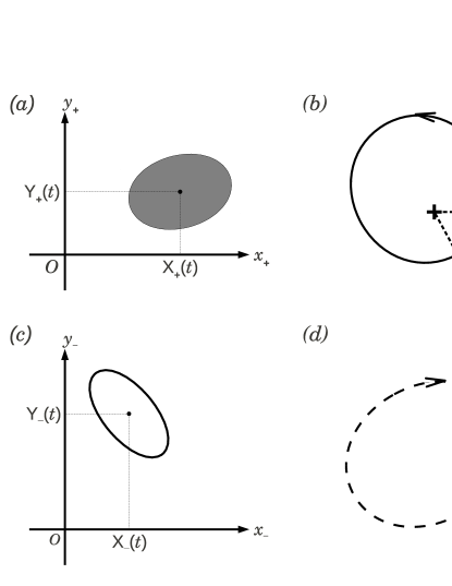
Figure 1: Distribution functions and centroid orbits: Panels ”a” and ”c” are schematic illustrations of the $\pm$ stellar distributions in the $\left(x_{\pm},y_{\pm}\right)$ phase spaces, respectively, at some given time. The elliptical patches indicate the regions populated by stars; each point in this phase space corresponds to a Keplerian orbit in physical space. The centroids of the ellipses, $\left(X_{\pm}(t),Y_{\pm}(t)\right)$, are marked by black dots, and the principal axes of the ellipses are given by the eigenvectors of the symmetric matrices, ${\bf Q}^{\pm}(t)\,$. Panels ”b” and ”d” are representations, in physical space, of the Keplerian orbits corresponding to the $\pm$ centroids. Note that the angles to the pericentre, $g_{\pm}^{c}=\mp\,\rm arctan{(X_{\pm}/Y_{\pm})}\,$; hence, for the distributions shown in panels ”a” and ”c”, we have $g_{+}^{c}<0\,$ and $g_{-}^{c}>0\,$.

The DFs $f^{\pm}(x_{\pm},y_{\pm},t)$ obey the CBEs of equations (36). By Jeans’ theorem (Binney & Tremaine, 2008), any function of the dynamical invariants is a solution of the CBE. Therefore we choose the $\pm$ DFs to be functions of the approximate invariants $J_{\pm}\,$:

$$f^{\pm}(x_{\pm},y_{\pm},t)\;=\;F^{\pm}\left(J_{\pm}\right)\,.$$ (50)

Schematic representations of DFs in the $\left(x_{\pm},y_{\pm}\right)$ phase-spaces, and of centroid orbits in physical space, are shown in Fig.(1). Here, we note the following important properties:

1. The DFs $F^{\pm}(J_{\pm})$ are assumed to have compact support over the interval $0\leq J_{\pm}\leq J_{\pm\rm max}\ll 1\,$.

2. $X_{\pm}(t)$ and $Y_{\pm}(t)$ are the coordinates of the centroids of the DFs, $\,F^{\pm}\left(J_{\pm}\right)\,,$ in the $\left(x_{\pm},y_{\pm}\right)$ phase spaces, respectively.

3. At any instant of time, the isocontours of the DFs are ellipses in the $\left(x_{\pm},y_{\pm}\right)$ phase spaces that are centered on $\left(X_{\pm}(t),Y_{\pm}(t)\right)$.

4. The shapes and orientations of the ellipses are described by the time–dependent, symmetric, positive definite matrices $\mbox{\boldmath$Q$}^{\pm}(t)$, which we will refer to as the shape matrices. Time evolution preserves ${\det}\left(\mbox{\boldmath$Q$}^{\pm}\right)$; we can choose ${\det}\left(\mbox{\boldmath$Q$}^{\pm}\right)=1\,$.

5. The zeroth and first moments of the DFs,

   $$M_{\pm}\;=\;{\int}_{0}^{J_{\pm\rm max}}2\pi dJ_{\pm}\,F^{\pm}(J_{\pm})\,;\qquad\quad{\sigma}^{2}_{\pm}\;=\;\frac{1}{M_{\pm}}{\int}_{0}^{J_{\pm\rm max}}2\pi dJ_{\pm}\,J_{\pm}\,F^{\pm}(J_{\pm})\,,$$ (51)

   are the disc masses and the squared dispersions (of eccentricities), respectively. Once the DFs have been specified, $M_{\pm}$ and $\sigma^{2}_{\pm}$ can be treated as constants.

6. We can now state precisely the conditions under which $F^{\pm}(J_{\pm})$ are approximate solutions. These DFs are good solutions when the dispersions in the eccentricities are much smaller than their centroid values; i.e. when

   $$0\;\leq\;{\sigma}_{\pm}\;\ll\;e_{\pm}\;\ll\;1\,,$$ (52)

   where $e_{\pm}$ is a typical value of $\sqrt{X^{2}_{\pm}+Y^{2}_{\pm}}\,$.

7. The total angular momentum in the two discs is

   $$\mathcal{L}_{\rm tot}\;=\;\sqrt{G\mbox{$M_{\bullet}$}a_{0}}\int\mbox{${\mathrm{d}}$}\ell\mbox{${\mathrm{d}}$}g\;\ell\,f^{+}\;\;+\;\;\sqrt{G\mbox{$M_{\bullet}$}a_{0}}\int\mbox{${\mathrm{d}}$}\ell\mbox{${\mathrm{d}}$}g\;\ell\,f^{-}\,,$$ (53)

   where $\ell$ is positive for $f^{+}$ with $\mbox{${\mathrm{d}}$}\ell\mbox{${\mathrm{d}}$}g=\mbox{${\mathrm{d}}$}x_{+}\mbox{${\mathrm{d}}$}y_{+}$, and $\ell$ is negative for $f^{-}\,$ with $\mbox{${\mathrm{d}}$}\ell\mbox{${\mathrm{d}}$}g=\mbox{${\mathrm{d}}$}x_{-}\mbox{${\mathrm{d}}$}y_{-}$. Using equations (14)—(16) and (39), we write

   $$\ell\;=\;\pm\left[1\;-\;\frac{1}{2}\left(x_{\pm}^{2}\,+\,y_{\pm}^{2}\right)\right]\;=\;\pm\left[1\;-\;\frac{1}{2}\left\{\left(\xi_{1\pm}\,+\,X_{\pm}\right)^{2}\;+\;\left(\xi_{2\pm}\,+\,Y_{\pm}\right)^{2}\right\}\right]$$ (54)

   For the DFs given in equation (50), $f^{\pm}(x_{\pm},y_{\pm},t)=F^{\pm}\left(J_{\pm}\right)$. When equation (54) is used, $\xi_{1\pm}$ and $\xi_{2\pm}$ contribute to the integral of equation (53) only at second order. These contributions are small, since the dispersion in eccentricities is much smaller than centroid values for these DFs. So we drop the dependences on $\xi_{1\pm}$ and $\xi_{2\pm}$ on the right side of equation (54), and set $x_{\pm}=X_{\pm}$ and $y_{\pm}=Y_{\pm}\,$. Using the definitions of $M_{\pm}$ given in the first of equations (51) above, we obtain

   $$\frac{\mathcal{L}_{\rm tot}}{\sqrt{G\mbox{$M_{\bullet}$}a_{0}}}\;=\;\left[M_{+}\,-\,M_{-}\right]\;-\;\frac{M_{+}}{2}\left[X_{+}^{2}\,+\,Y_{+}^{2}\right]\;+\;\frac{M_{-}}{2}\left[X_{-}^{2}\,+\,Y_{-}^{2}\right]\;+\;O\left({\sigma}_{\pm}^{2}/e_{\pm}^{2}\right)\,.$$ (55)

   The first term on the right side is the contribution from the $\pm$ discs if they were circular; the second term is the decrement due to the centroid eccentricity of the $+$ disc; the third term is a similar and oppositely signed contribution from the $-$ disc.

We need to compute the coefficients $\left(A_{\pm},B_{\pm},C_{\pm},D_{\pm},E_{\pm},F_{\pm},G_{\pm},K_{\pm}\,\right)$, by substituting equation (50) for the $\pm$ DFs in equations (34). Similar to the treatment of the angular momentum of the discs given above, we set $x_{\pm}=X_{\pm}$ and $y_{\pm}=Y_{\pm}\,$. Then, it is straightforward to express the coefficients as functions of the centroid coordinates, $\left[X_{\pm}(t)\,,\,Y_{\pm}(t)\right]$:

$$A_{\pm} = -\,2M\alpha\;-\;2M_{\pm}\left[(\gamma+\lambda){X}_{\pm}^{2}+\gamma{Y}_{\pm}^{2}\right]\;-\;2M_{\mp}\left[(\gamma+\lambda){X}_{\mp}^{2}+\gamma{Y}_{\mp}^{2}\right]$$

$$B_{\pm} = -\,2\lambda M_{\pm}{X}_{\pm}{Y}_{\pm}\;+\;2\lambda M_{\mp}{X}_{\mp}{Y}_{\mp}$$

$$C_{\pm} = -\,2M\alpha\;-\;2M_{\pm}\left[\gamma{X}_{\pm}^{2}+(\gamma+\lambda){Y}_{\pm}^{2}\right]\;-\;2M_{\mp}\left[\gamma{X}_{\mp}^{2}+(\gamma+\lambda){Y}_{\mp}^{2}\right]$$

$$D_{\pm} = -\beta M_{\pm}X_{\pm}\,-\,\left(\kappa-\frac{\beta}{8}\right)M_{\pm}\left[{X}_{\pm}^{3}+X_{\pm}Y_{\pm}^{2}\right]\,+\,\beta M_{\mp}X_{\mp}\,+\,\left(\kappa-\frac{\beta}{8}\right)M_{\mp}\left[{X}_{\mp}^{3}+X_{\mp}Y_{\mp}^{2}\right]$$

$$E_{\pm} = -\,\beta M_{\pm}Y_{\pm}\;-\;\left(\kappa-\frac{\beta}{8}\right)M_{\pm}\left[{Y}_{\pm}^{3}+X_{\pm}^{2}Y_{\pm}\right]\;-\;\beta M_{\mp}Y_{\mp}\;-\;\left(\kappa-\frac{\beta}{8}\right)M_{\mp}\left[{Y}_{\mp}^{3}+X_{\mp}^{2}Y_{\mp}\right]$$

$$F_{\pm} = -\left(\kappa-\frac{\beta}{8}\right)\left[M_{\pm}X_{\pm}-M_{\mp}X_{\mp}\right]$$

$$G_{\pm} = -\left(\kappa-\frac{\beta}{8}\right)\left[M_{\pm}Y_{\pm}+M_{\mp}Y_{\mp}\right]$$

$$K_{\pm} = -\left(\chi-\frac{\alpha}{4}\right)M\,.$$ (56)

The centroid coordinates obey:

$$\frac{\mbox{${\mathrm{d}}$}X_{\pm}}{\mbox{${\mathrm{d}}$}t} = B_{\pm}X_{\pm}\;+\;C_{\pm}Y_{\pm}\;+\;E_{\pm}\;+\;2F_{\pm}X_{\pm}Y_{\pm}\;+\;G_{\pm}\left(X_{\pm}^{2}+3Y_{\pm}^{2}\right)\;+\;4K_{\pm}\left(Y_{\pm}^{3}+Y_{\pm}X_{\pm}^{2}\right)$$

$$\frac{\mbox{${\mathrm{d}}$}Y_{\pm}}{\mbox{${\mathrm{d}}$}t} = -A_{\pm}X_{\pm}-B_{\pm}Y_{\pm}-D_{\pm}-F_{\pm}\left(3X_{\pm}^{2}+Y_{\pm}^{2}\right)-2G_{\pm}X_{\pm}Y_{\pm}-4K_{\pm}\left(X_{\pm}^{3}+X_{\pm}Y_{\pm}^{2}\right)\,.$$

These are a set of 4 autonomous first order ODEs with cubic nonlinearity. The shape matrices obey the following first order matrix ODEs:

$$\frac{d\mbox{\boldmath$Q$}^{\pm}}{dt}\;=\;-\,\left(\mbox{\boldmath$T$}^{\pm}\right)^{\rm T}\mbox{\boldmath$Q$}^{\pm}\;-\;\mbox{\boldmath$Q$}^{\pm}\,\mbox{\boldmath$T$}^{\pm}\,;\qquad\quad\mbox{\boldmath$T$}^{\pm}(t)\;=\;\left(\begin{array}[]{lr}\;B_{\rm t\pm}&C_{\rm t\pm}\\[20.00003pt] -\,A_{\rm t\pm}&\;-\,B_{\rm t\pm}\end{array}\right)\,,$$ (58)

where

$$A_{\rm t\pm} = A_{\pm}\;+\;6F_{\pm}X_{\pm}\;+\;2G_{\pm}Y_{\pm}\;+\;4K_{\pm}\left(Y_{\pm}^{2}+3X_{\pm}^{2}\right)$$

$$B_{\rm t\pm} = B_{\pm}\;+\;2F_{\pm}Y_{\pm}\;+\;2G_{\pm}X_{\pm}\;+\;8K_{\pm}X_{\pm}Y_{\pm}$$

$$C_{\rm t\pm} = C_{\pm}\;+\;2F_{\pm}X_{\pm}\;+\;6G_{\pm}Y_{\pm}\;+\;4K_{\pm}\left(X_{\pm}^{2}+3Y_{\pm}^{2}\right)\,.$$ (59)

Since $\mbox{\boldmath$T$}^{\pm}(t)$ are traceless matrices, $\det\left[\mbox{\boldmath$Q$}^{\pm}(t)\right]$ is a conserved quantity; without loss of generality, we can choose $\det\left[\mbox{\boldmath$Q$}^{\pm}(0)\right]=1\,$. The matrix $T$ depends on the centroid coordinates, so the matrix equations for $Q$, while linear, are driven by centroid evolution. Equations (56)—(59) determine the self–consistent centroid and shape dynamics of DFs describing the counter–rotating discs.

5 Counter–rotating discs: centroid dynamics

As shown above, in the limit $0\,\leq\,{\sigma}_{\pm}\,\ll\,e_{\pm}\,\ll\,1\,,$ shape dynamics is driven by centroid dynamics, and consists of area preserving evolution of the shape and orientation of the elliptical isocontours of the DFs, with no feedback on centroids. In what follows, and with the understanding that shape can be recovered easily from centroids as and when required by a given application, we drop any further reference to shape dynamics, and focus our attention on the nonlinear evolution of the centroids.

5.1 Integrability

The centroid equations (LABEL:eqs:xypm) are a set of 4 autonomous first order ODEs with cubic nonlinearity. Quite remarkably, it turns out that they describe a non linear, yet integrable, system. This happens because of the underlying Hamiltonian structure and the presence of a second conserved quantity. Let us define new rescaled variables $\left(u_{\pm},v_{\pm}\right)$:

$$u_{\pm} = \sqrt{{\mu}_{\pm}}\;X_{\pm}\,,\qquad v_{\pm}\;=\;\sqrt{{\mu}_{\pm}}\;Y_{\pm}$$

$${\mu}_{\pm} = \frac{M_{\pm}}{M}\,,\qquad\mbox{so}\quad\left({\mu}_{+}\,+\,{\mu}_{-}\right)\;=\;1\,.$$ (60)

A lengthy yet straightforward calculation shows that the centroid equations (LABEL:eqs:xypm) are equivalent to the following two degree–of–freedom system Hamiltonian system, with coordinates $u_{\pm}$ and momenta $v_{\pm}\,$:

$$\frac{\mbox{${\mathrm{d}}$}u_{+}}{\mbox{${\mathrm{d}}$}t} = \frac{\partial{\mathcal{H}}}{\partial v_{+}}\,,\qquad\frac{\mbox{${\mathrm{d}}$}v_{+}}{\mbox{${\mathrm{d}}$}t}\;=\;-\frac{\partial{\mathcal{H}}}{\partial u_{+}}\,;\qquad\quad\frac{\mbox{${\mathrm{d}}$}u_{-}}{\mbox{${\mathrm{d}}$}t}\;=\;\frac{\partial{\mathcal{H}}}{\partial v_{-}}\,,\qquad\frac{\mbox{${\mathrm{d}}$}v_{-}}{\mbox{${\mathrm{d}}$}t}\;=\;-\frac{\partial{\mathcal{H}}}{\partial u_{-}}\,,$$

$${\mathcal{H}} = -\left(\frac{\beta M{\mu}_{+}}{2}\,+\,M\alpha\right)\left[u_{+}^{2}\,+\,v_{+}^{2}\right]\;-\;\left(\frac{\beta M{\mu}_{-}}{2}\,+\,M\alpha\right)\left[u_{-}^{2}\,+\,v_{-}^{2}\right]$$ (61)

$$+\;\beta M\sqrt{{\mu}_{+}{\mu}_{-}}\,\left[u_{+}u_{-}\,-\,v_{+}v_{-}\right]$$

$$-\left(\frac{\gamma+\lambda}{2}\,+\,\frac{4\chi-\alpha}{4\mu_{+}}\,+\,\kappa\,-\,\frac{\beta}{8}\right)M\left[u_{+}^{2}\,+\,v_{+}^{2}\right]^{2}$$

$$-\left(\frac{\gamma+\lambda}{2}\,+\,\frac{4\chi-\alpha}{4\mu_{-}}\,+\,\kappa\,-\,\frac{\beta}{8}\right)M\left[u_{-}^{2}\,+\,v_{-}^{2}\right]^{2}$$

$$-\;\lambda M\left[u_{+}u_{-}\,-\,v_{+}v_{-}\right]^{2}\;-\;\gamma M\left[\left(u_{+}^{2}+v_{+}^{2}\right)\left(u_{-}^{2}+v_{-}^{2}\right)\right]$$

$$+\;\left(\kappa-\frac{\beta}{8}\right)M\left[u_{+}u_{-}\,-\,v_{+}v_{-}\right]\left[\sqrt{\frac{{\mu}_{+}}{{\mu}_{-}}}\left(u_{-}^{2}\,+\,v_{-}^{2}\right)\,+\,\sqrt{\frac{{\mu}_{-}}{{\mu}_{+}}}\left(u_{+}^{2}\,+\,v_{+}^{2}\right)\right]\,,$$

where ${\mathcal{H}}\left(u_{+},u_{-},v_{+},v_{+}\right)$ is the Hamiltonian for the two degree–of–freedom system with coordinates $u_{\pm}$ and momenta $v_{\pm}\,$. Since ${\mathcal{H}}$ is independent of time, it is conserved. It is straightforward to verify that equations (61) also conserve the total angular momentum defined in equation (55). Dropping the first term, we write the second conserved quantity as

$${\mathcal{L}}\;=\;\frac{u_{+}^{2}\,+\,v_{+}^{2}}{4}\;-\;\frac{u_{-}^{2}\,+\,v_{-}^{2}}{4}\,.$$ (62)

This quantity is a measure of the amount by which the angular momentum is lower than the maximum value it can attain when the centroid eccentricities are zero; for brevity we shall henceforth refer to ${\mathcal{L}}$ as the angular momentum.

Since this two degree–of–freedom system has two independent conserved quantities, ${\mathcal{H}}$ and ${\mathcal{L}}$, it is integrable. We will explore the non linear dynamics of this system, after examining the linear instability of zero eccentricity discs.

5.2 Linear instability of zero eccentricity discs

The zero eccentricity state, $u_{\pm}=v_{\pm}=0$ which has ${\mathcal{L}}=0\,$, is an equilibrium state of the dynamics governed by ${\mathcal{H}}$. Here we determine the conditions under which this equilibrium is unstable to small perturbations. The linearized equations obeyed by infinitesimal perturbations are:

$$\frac{\mbox{${\mathrm{d}}$}u_{+}}{\mbox{${\mathrm{d}}$}t} = -w_{+}v_{+}\;-\;w_{c}v_{-}\,,\qquad\quad\frac{\mbox{${\mathrm{d}}$}v_{+}}{\mbox{${\mathrm{d}}$}t}\;=\;w_{+}u_{+}\;-\;w_{c}u_{-}\,;$$

$$\frac{\mbox{${\mathrm{d}}$}u_{-}}{\mbox{${\mathrm{d}}$}t} = -w_{-}v_{-}\;-\;w_{c}v_{+}\,,\qquad\quad\frac{\mbox{${\mathrm{d}}$}v_{-}}{\mbox{${\mathrm{d}}$}t}\;=\;w_{-}u_{-}\;-\;w_{c}u_{+}\,,$$ (63)

where $w_{\pm}=\left(2M\alpha\,+\,\beta M_{\pm}\right)\,$, and $w_{c}=\beta\sqrt{M_{+}M_{-}}\;$ are constants. It is readily verified that this linearized system conserves ${\mathcal{L}}$. To solve these equations let us define the complex variables:

$$z_{+}\;=\;u_{+}\;+\;{\mathrm{i}}\,v_{+}\,,\qquad\quad z_{-}\;=\;v_{-}\;+\;{\mathrm{i}}\,u_{-}\,,$$ (64)

in terms of which equations (63) reduce to:

$$\frac{\mbox{${\mathrm{d}}$}z_{+}}{\mbox{${\mathrm{d}}$}t}\;=\;{\mathrm{i}}\,w_{+}z_{+}\;-\;w_{c}z_{-}\,,\qquad\quad\frac{\mbox{${\mathrm{d}}$}z_{-}}{\mbox{${\mathrm{d}}$}t}\;=\;-{\mathrm{i}}\,w_{-}z_{-}\;-\;w_{c}z_{+}\,.$$ (65)

Note that the asymmetry in Eqs. (65) is inherited from the asymmetry in the definition of $z_{\pm}$ in Eqs. (64). Looking for normal modes, $z_{\pm}=Z_{\pm}{\mathrm{e}}^{st}\,$, we obtain and solve a quadratic characteristic equation for the two eigenvalues:

$$s\;=\;\frac{{\mathrm{i}}}{2}\left({w_{+}-w_{-}}\right)\;\pm\;\frac{1}{2}\sqrt{4\,w_{c}^{2}\,-\,\left(w_{+}+w_{-}\right)^{2}}\;\;.$$ (66)

There is a growing solution when $4w_{c}^{2}>\left(w_{+}+w_{-}\right)^{2}$. Thus the zero eccentricity equilibrium, $u_{\pm}=v_{\pm}=0\,$, is unstable (overstable) when

$${\mu_{+}}{\mu_{-}}\;>\;\frac{1}{4}{\left(1+\frac{4\alpha}{\beta}\right)}^{2}\,.$$ (67)

Figure 2: Linear Stability of the zero angular momentum equilibrium: Left: Curve of critical values in the plane of mass ratio $\mu$ and dimensionless softening $r=b/a_{0}$ above which the centroids of the prograde and retrograde population are unstable to eccentricity growth. Right: The real parts of the eigenvalues given in equations (66), as a function of $\mu$ for $r=0.1\,$. Instability sets in for $\mu\geq\mu_{\rm crit}\simeq 0.4436\,$.

Using the definitions of $\alpha$ and $\beta$ given in the Appendix A, we display the stability criterion of equation (67) in Fig.(2) by plotting the mass ratio, $\mu=M_{-}/M_{+}\,$, versus the dimensionless softening, $r=b/a_{0}\,$. For a given softening, there is a critical value of the mass ratio (which decreases with increasing softening) above which the zero–eccentricity equilibrium is unstable. Conversely, for a given mass ratio, there is a critical value of the softening (which increases with decreasing mass ratio) above which the zero–eccentricity equilibrium is unstable. In the right panel of Fig.(2) we plot the real parts of the eigenvalues given in equations (66), as a function of $\mu$ for $r=0.1\,$. When $\mu\leq\mu_{\rm crit}\simeq 0.4436\,$, the eigenvalues are both imaginary, corresponding to normal modes describing steadily precessing discs of fixed centroid eccentricities. Both growing and damped solutions are allowed when $\mu>\mu_{\rm crit}\,$. The growing (damped) solution describes discs whose eccentricities grow (damp) as they precess steadily.

Since ${\mathcal{L}}$ is conserved, the instability operates through exchange of angular momentum between the prograde and retrograde discs. When the prograde disc gives some angular momentum to the retrograde disc, both discs increase their eccentricities. As is well–known (Miller, 1971; Binney & Tremaine, 2008), the softening length mimics the epicyclic radius of stars on nearly circular orbits. For this exchange to be self-reinforcing, for the instability to kick in, the mass ratio has to be large enough for $\pm$ disk self-gravity to overcome the effective “heat” due to softening (a process which is similar to the one driving the radial orbit instability (Lynden-Bell, 1979)).

5.3 Nonlinear dynamics

As discussed earlier centroid dynamics is integrable, because it is a two degree–of–freedom system (4–dimensional phase space) with two independent conserved quantities. We now use the conservation of the angular momentum of equation (62) to convert the problem into a Hamiltonian system of one degree–of–freedom system. We achieve this through two canonical transformations to new variables. First, we pass from $\left(u_{\pm},v_{\pm}\right)$ to new action–angle variables, $\left(L_{\pm},\psi_{\pm}\right)$:

$$u_{+} = \sqrt{2{L}_{+}}\,\sin{\psi}_{+}\,,\qquad\quad v_{+}\;=\;\sqrt{2{L}_{+}}\,\cos{\psi}_{+}\;;$$

$$u_{-} = \sqrt{2{L}_{-}}\,\sin{\psi}_{-}\,,\qquad\quad v_{-}\;=\;\sqrt{2{L}_{-}}\,\cos{\psi}_{-}\;.$$ (68)

Written in terms of the new variables, the Hamiltonian of equations (61) becomes:

$${\mathcal{H}} = -\,w_{+}{L}_{+}\;-\;w_{-}{L}_{-}\;-\;2w_{c}\sqrt{{L}_{+}{L}_{-}}\,\cos\left({\psi}_{+}\,+\,{\psi}_{-}\right)$$ (69)

$$-\,4{\eta}_{+}{L}_{+}^{2}\;-\;4{\eta}_{-}{L}_{-}^{2}\;-\;4\left(\kappa-\frac{\beta}{8}\right)M\sqrt{{L}_{+}{L}_{-}}\,\cos\left({\psi}_{+}+{\psi}_{-}\right)\left[\sqrt{\frac{{\mu}_{+}}{{\mu}_{-}}}\,{L}_{-}\,+\,\sqrt{\frac{{\mu}_{-}}{{\mu}_{+}}}\,{L}_{+}\right]$$

$$-\,4\lambda M{L}_{+}{L}_{-}\,{\cos}^{2}\left({\psi}_{+}+{\psi}_{-}\right)\;-\;4\gamma M{L}_{+}{L}_{-}\,,$$

where the new constants, $\eta_{\pm}$, are defined by:

$${\eta}_{\pm}\;=\;\left(\frac{\gamma+\lambda}{2}\,+\,\frac{4\chi-\alpha}{4\mu_{\pm}}\,+\,\kappa\,-\,\frac{\beta}{8}\right)M\,.$$ (70)

The angles ${\psi}_{+}$ and ${\psi}_{-}$ appear only in the combination $\left({\psi}_{+}+{\psi}_{-}\right)$. So we transform to new action–angle variables, $\left(\Sigma,\Theta\right)$ and $\left({\mathcal{L}},\vartheta\right)$, defined through the generating function, ${\mathcal{S}}\left({\mathcal{L}},\Sigma,{\psi}_{+},{\psi}_{-}\right)=\left({\psi}_{+}+{\psi}_{-}\right)\Sigma\,+\,\left({\psi}_{+}-{\psi}_{-}\right){\mathcal{L}}\,$. Then,

$${L}_{+} = \Sigma\;+\;{\mathcal{L}}\,,\qquad\quad{L}_{-}\;=\;\Sigma\;-\;{\mathcal{L}}\,;$$

$$\vartheta = {\psi}_{+}\;-\;{\psi}_{-}\,,\qquad\quad\Theta\;=\;{\psi}_{+}\;+\;{\psi}_{-}\,.$$ (71)

When expressed in terms of the new variables, the Hamiltonian becomes:

$${\mathcal{H}} = -\,\left(w_{+}+w_{-}\right)\Sigma\;-\;\left(w_{+}-w_{-}\right){\mathcal{L}}\;-\;2w_{c}\sqrt{{\Sigma}^{2}\,-\,{\mathcal{L}}^{2}}\,\cos\Theta$$ (72)

$$-\,4\left({\eta}_{+}+{\eta}_{-}\right){\Sigma}^{2}\;-\;8({\eta}_{+}-{\eta}_{-})\;{\Sigma}{\mathcal{L}}\;-\;4\left({\eta}_{+}+{\eta}_{-}\right){\mathcal{L}}^{2}$$

$$-\,4\left(\kappa-\frac{\beta}{8}\right)M\sqrt{{\Sigma}^{2}-{\mathcal{L}}^{2}}\,\left[\left(\sqrt{\frac{\mu_{-}}{\mu_{+}}}+\sqrt{\frac{\mu_{+}}{\mu_{-}}}\right)\Sigma\,+\,\left(\sqrt{\frac{{\mu}_{-}}{{\mu}_{+}}}-\sqrt{\frac{{\mu}_{+}}{{\mu}_{-}}}\right){\mathcal{L}}\right]\,\cos\Theta$$

$$-\,4\gamma M\left({\Sigma}^{2}\,-\,{\mathcal{L}}^{2}\right)\;-\;4\lambda M\left({\Sigma}^{2}-{\mathcal{L}}^{2}\right)\,{\cos}^{2}\Theta\,.$$

Since ${\mathcal{H}}$ is independent of $\vartheta$, its conjugate momentum ${\mathcal{L}}$ is conserved. Hence ${\mathcal{L}}$ may be treated as a constant parameter occurring in ${\mathcal{H}}$, which can be thought of as a Hamiltonian describing the one degree–of–freedom Hamiltonian with coordinate $\Theta$ and momentum $\Sigma$.

The global structure of dynamics in the $\left(\Theta,\Sigma\right)$ phase space is most easily visualized by plotting the level curves of ${\mathcal{H}}$ for different values of the constant parameter ${\mathcal{L}}$. It seems simplest to label the axes of the figures, using the “cartesian–type” canonical variables:

$$U\;=\;\sqrt{2\left(\Sigma-{\mathcal{L}}\right)}\,\sin\Theta\,,\qquad\quad V\;=\;\sqrt{2\left(\Sigma-{\mathcal{L}}\right)}\,\cos\Theta\,,$$ (73)

where $U$ and $V$ are new coordinates and momenta, respectively. Before we discuss the phase space structure, it is useful to interpret the canonical variables in terms of physical quantities related to the centroids of the prograde and retrograde populations:

• $\sqrt{U^{2}+V^{2}}=\sqrt{2(\Sigma-{\mathcal{L}})}=\sqrt{2{L}_{-}}=\sqrt{u_{-}^{2}+v_{-}^{2}}$ is proportional to the centroid eccentricity of the retrograde ring.

• $U=V=0$ represents the zero eccentricity state; it is an equilibrium for ${\mathcal{L}}=0$, but not otherwise.

• $\Theta=\left({\psi}_{+}\,+\,{\psi}_{-}\right)=\left(g^{\rm cent}_{-}\,-\,g^{\rm cent}_{+}\right)$ is the difference between the periapse angles of the centroids of the retrograde and prograde populations. Since we also have $\Theta=\arctan{(U/V)}$, we note that:

  • $U=0$ and $V<0$ implies that $\left(g^{\rm cent}_{-}\,-\,g^{\rm cent}_{+}\right)=\pi$, corresponding to eccentric $\pm$ discs with anti–aligned periapses.

  • $U=0$ and $V>0$ implies that $\left(g^{\rm cent}_{-}\,-\,g^{\rm cent}_{+}\right)=0$, corresponding to eccentric $\pm$ discs with aligned periapses.

Before we begin, we need to determine the parameters — other than ${\mathcal{L}}$ – that control the dynamics. We first note that the constants $w_{\pm}$, $w_{c}$ and $\eta_{\pm}$ are all proportional to the total mass, $M$, in the $\pm$ discs. Each of the parameters $\left(\alpha,\beta,\gamma,\lambda,\kappa,\chi\right)$ is proportional to $a_{0}^{-3/2}\,$, where $a_{0}$ is the semi–major axis; these parameters are also functions of the dimensionless softening parameter $r=b/a_{0}\,$, but the dependences are not so simple. Therefore, every term on the right side of equation (72) is proportional to $Ma_{0}^{-3/2}\,$, so this combination of constants determines only the rate at which a phase trajectory is traversed. For the purposes of investigating the geometry of phase space, we may set $Ma_{0}^{-3/2}$ equal to unity. The dimensionless masses, $\mu_{+}=(M_{+}/M)$ and $\mu_{-}=(M_{-}/M)$, can both be expressed in terms of the dimensionless mass ratio, $\mu=(M_{-}/M_{+})\,$. Therefore, we are left with the three dimensionless parameters $\left({\mathcal{L}},r,\mu\right)$, which control the dynamics generated by ${\mathcal{H}}\,$.

5.3.1 Dynamics when ${\mathcal{L}}=0$

When ${\mathcal{L}}=0$, the prograde and retrograde discs have equal amounts of mass–weighted centroid eccentricities. We have already studied the linear instability of the zero eccentricity equilibrium in § 5.2. At a fixed value of $r$, there is a critical value of the mass ratio $\mu$ above which the instability sets it. When $r=0.1$, this critical mass ratio is ${\mu}_{\rm crit}\simeq 0.4436$, which corresponds to about $70\%$ of the disc mass in the prograde component and the remaining mass in the retrograde component. Here we explore the structure of nonlinear centroid dynamics as $\mu$ is varied, with both ${\mathcal{L}}$ and $r$ held fixed.

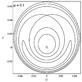
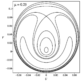
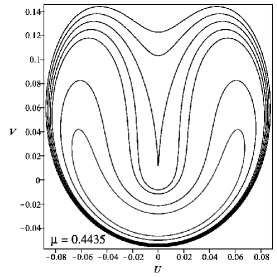
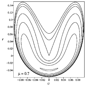
Figure 3: Phase portraits for four different values of $\mu$, when ${\mathcal{L}}=0\,$ and $r=0.1\,$.

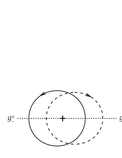
Figure 4: Snapshot of the $\pm$ centroid orbits in physical space corresponding to the stable, precessing equilibrium P1 $(U=0,V\simeq-0.04)$ in the bottom–right panel of Fig.(3). The cross marks the location of the central mass, which is at the common focus of both the prograde (solid) and the retrograde (dashed) centroid orbits. The eccentricities of the $\pm$ orbits are $0.05$ and $0.06$, respectively, and have been greatly exaggerated in the figures. Note that the $\pm$ periapses are anti–aligned.

Fig.(3) displays the level curves of ${\mathcal{H}}$ in the $\left(U,V\right)$ phase space for four different values of $\mu$, when ${\mathcal{L}}=0\,$ and $r=0.1\,$. Phase flows occur along these level curves. Some noteworthy features are:

• For $\mu\leq{\mu}_{\rm crit}$, the zero–eccentricity equilibrium $P_{2}=(0,0)$ is stable; but there are also two additional equilibria, $P_{1}=\left(0,V_{1}\right)$ and $P_{3}=\left(0,V_{3}\right)$.

• $P_{1}$ is stable: it has $U=0\,$ and $V_{1}<0$, which corresponds to steadily precessing eccentric $\pm$ discs with anti–aligned periapses.

• $P_{3}$ is unstable: it has $U=0\,$ and $V_{3}>0$, which corresponds to steadily precessing eccentric $\pm$ discs with aligned periapses.

• When $\mu$ exceeds $\mu_{\rm crit}$, the zero–eccentricity equilibrium $P_{2}$ goes unstable by merging with the unstable equilibrium $P_{3}$. Small perturbations about $P_{2}$ now exhibit large variations in eccentricity, with phase space trajectories that take them on an excursion around the stable equilibrium $P_{1}\,$. A schematic view in physical space of anti-aligned centroid orbits at $P_{1}$ is shown in Fig.(4).

• $P_{1}$ remains stable for all values of $\mu\,$.

• The bifurcation of equilibria as a function of $\mu$, at fixed $r\,$, is shown in Fig.(5). The plot reflects transition across ${\mu}_{\rm crit}$, with the two equilibria $P_{2}$ and $P_{3}$ merging to form an unstable equilibrium, along with the continuing sequence of the stable equilibrium $P_{1}\,$.

• Further increase in $\mu$ does not alter the equilibrium structure. However, there are larger excursions in eccentricity, so much so, that the conditions under which the model works can be in question.

Figure 5: Bifurcation of equilibria: Plot of the values of the $V$–coordinates of the stable and unstable equilibria, as functions of the mass ratio $\mu$. Stable/unstable equilibria are shown in solid/dashed lines.

5.3.2 Dynamics when ${\mathcal{L}}\neq 0$

When ${\mathcal{L}}\neq 0$, the mass–weighted centroid eccentricities of the prograde and retrograde discs are unequal. Without loss of generality, we assume that ${\mathcal{L}}\geq 0$; in other words, we assume that the mass–weighted centroid eccentricity of the prograde disc is greater than that of the retrograde disc. We follow the equilibria and their bifurcations as ${\mathcal{L}}$ is increased, at fixed $\mu$ and $r$. Some noteworthy features of the phase–space evolution, shown in Fig.(6), are:

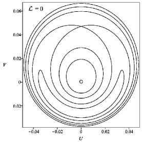
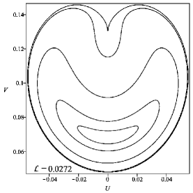
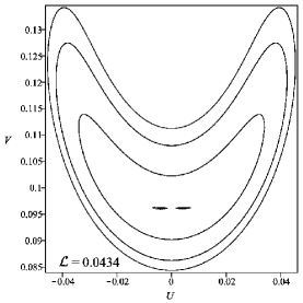
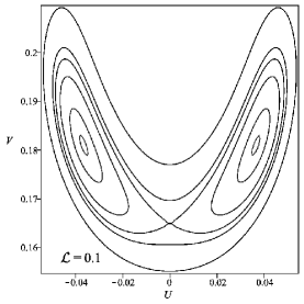
Figure 6: Phase–space evolution with increasing value of ${\mathcal{L}}$.

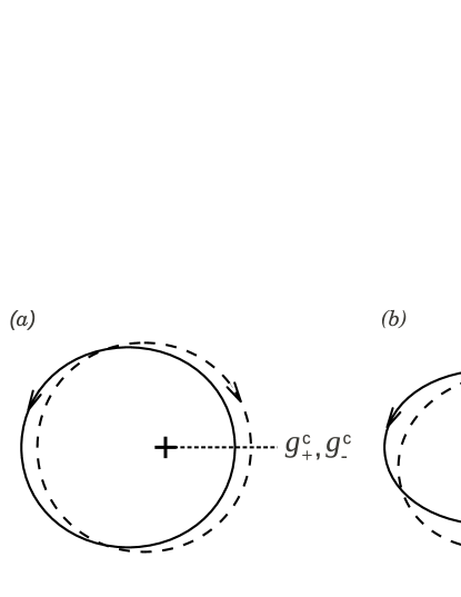
Figure 7: Snapshots of the $\pm$ centroid orbits in physical space, corresponding to the stable (precessing) equilibrium P1 for two different cases. The cross marks the location of the central mass, which is at the common focus of both the prograde (solid) and the retrograde (dashed) centroid orbits. Panel ”a” corresponds to top–right panel of Fig.(6) ($\cal{L}$= 0.0272), when P1 $(U=0,V\simeq 0.07)$ is still a stable equilibrium before bifurcation. The eccentricities of the $\pm$ orbits are $0.35$ and $0.2$, respectively. Note that the $\pm$ periapses are aligned. Panel ”b” corresponds to the bottom–right panel of Figure 4 ($\cal{L}$= 0.0272), when P1 has bifurcated into two stable equilibria, P1a and P1b, which are at $U\simeq\pm 0.04$ and $V\simeq 0.18$; we show orbits for P1a . The eccentricities of the $\pm$ orbits are $0.65$ and $0.55$, respectively. Note that the $\pm$ periapses are mis-aligned, with the pericentre of the “-” orbit leading the pericentre of the “+” orbit by about $12.5\deg$ (for P1b, the pericentre of the “-” orbit would lag the pericentre of the “+” orbit by the same amount.

• As we have seen earlier, when ${\mathcal{L}}=0\,$, there is a qualitative change in the phase portrait when $\mu$ is smaller or larger than $\mu_{\rm crit}\,$, for some chosen value of $r$. For $r=0.1$, $\mu=0.1<\mu_{\rm crit}\,$ so the zero–eccentricity equilibrium: we have three equilibria; two stable ($P_{1}$, $P_{2}$) and one unstable ($P_{3}$), as discussed above.

• With increasing ${\mathcal{L}}$, $P_{2}$ (which was initially at the origin) shifts continuously to higher eccentricity with $U_{2}=0$ and $V_{2}>0\,$, corresponding to steadily precessing eccentric $\pm$ discs with aligned periapses. At the critical value of ${\mathcal{L}}\simeq 0.0271\,$, $P_{2}$ and $P_{3}$ collide.

• All through, $P_{1}$ remains stable with $U_{1}=0\,$. However, as ${\mathcal{L}}$ increases, $V_{1}$ also increases and, near ${\mathcal{L}}\simeq 0.0031\,$, $V_{1}$ becomes positive from its initially negative value; thus the corresponding stable, steadily precessing eccentric $\pm$ discs switch from anti–aligned to aligned periapses.

• With further increase in ${\mathcal{L}}$, $P_{1}$ remains stable with $U_{1}=0$ and increasing $V_{1}$ until we hit another critical value, ${\mathcal{L}}\simeq 0.0433$ . At this value of ${\mathcal{L}}$, $P_{1}$ becomes unstable and, in a pitchfork–like bifurcation, there emerge two stable and non–aligned equilibria. The remarkable feature of these new equilibria is that they are neither aligned nor anti–aligned. This suggests that, for large enough values of ${\mathcal{L}}$, the stable, uniformly precessing counter–rotating discs have periapses that are neither aligned nor anti–aligned. The transition from aligned to non-aligned stable equilibria at the bifurcation is illustrated in Fig.(7) with centroid orbits in physical space, at $P_{1}$ before the bifurcation, and at one of its two stable offsprings after.

• Increasing ${\mathcal{L}}$ still further maintains the equilibrium structure with the stable equilibria increasing in eccentricity and misalignment, in a fashion reminiscent of the displacement of an unstable bead on a rapidly spinning hoop.

• In the left panel of Fig.(8), we show the on–axis equilibria, the eventual merging of $P_{2}$ and $P_{3}$, followed by the loss of stability of $P_{1}$. In the right panel, we follow the bifurcation from $P_{1}$ (now unstable) of the two stable, non–aligned equilibria.

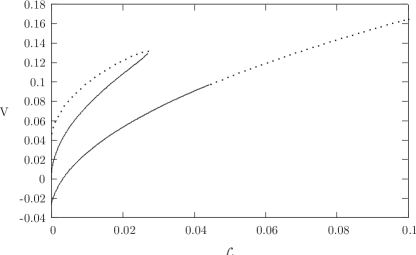
Figure 8: Uniformly precessing configurations for ${\mathcal{L}}\neq 0\,$. Left: Plot of the $Y$–coordinates of the equilibria as functions of ${\mathcal{L}}$, for the on–axis ($U=0$) equilibria which correspond to aligned and anti–aligned periapses. Stable/unstable equilibria are shown in solid/dashed lines, unstable. Two critical values of ${\mathcal{L}}$ are apparent: ${\mathcal{L}}\simeq 0.0271$, at which stable and unstable equilibria merge; ${\mathcal{L}}\simeq 0.0433$, at which $P_{1}$ becomes unstable, giving birth to non–aligned equilibria (with $U\neq 0\,$). Also apparent is the transition, at ${\mathcal{L}}\simeq 0.0031$, of the $P_{1}$, from being an equilibrium with stable anti–aligned periapses ($V_{1}<0\,$) to stable aligned periapses ($V_{1}>0\,$). Right: The bifurcation of the $P_{1}$, from being an aligned on–axis equilibrium to non–aligned equilibria.

6 Summary and conclusions

We have formulated the problem of the collisionless, self–consistent dynamics of nearly Keplerian star clusters around a massive black hole. Averaging over the fast Keplerian phase, we used the result that the semi–major axes of the stellar orbits are nearly conserved quantities. Hence each stellar orbit may be imagined to be a Gaussian ring, of fixed semi–major axis, whose shape and orientation changes over time scales that are longer than the Kepler orbital times. Since the semi–major axis of each stellar orbit is constant, and the orbital phase unimportant, the phase space in which the slow dynamics of an individual orbit occurs is four–dimensional. In terms of the Delaunay actions–angle variables, the two actions are the magnitude of the angular momentum and the $z$–component of the angular momentum, with corresponding angles being the argument of the periapse and the longitude of the ascending node. The star cluster was described by a distribution function (DF), which is a function of five variables: the four action–angle variables described above, and the constant semi–major axis which can differ from star to star. We presented the collisionless Boltzmann equation (CBE), which governs the self–consistent slow dynamics of the star cluster. The Hamiltonian determining this dynamics is the orbit–averaged gravitational potential energy between the stars; it is determined by integrating a softened Keplerian potential over the orbital phases of both rings (thereby forming a “ring–ring interaction function”), and then integrating this over all of phase space, suitably weighted by the DF.

The goal of this paper is to explore the counter–rotating instability. To this end, we considered the CBE for razor–thin, planar discs; in this case, at each value of the semi–major axis, the phase space is two dimensional, topologically equivalent to the 2–sphere. Then we considered the counter–rotating discs as two separate collisionless populations of stars, the prograde (or “$+$”) disc and the retrograde (or “$-$” disc). For convenience, we assumed that all the prograde stars have the same semi–major axes and all the retrograde stars have the same semi–major axes. Thus the total phase space is the direct sum of two 2–spheres; one for the prograde disc, the other for the retrograde disc. We then wrote down two separate $\pm$ DFs which obeyed two separate $\pm$ CBEs, governed by two separate $\pm$ Hamiltonians. Since the $\pm$ populations are gravitationally coupled, each of the $\pm$ Hamiltonians depends on both the $\pm$ DFs. When the discs are composed of stellar orbits of small eccentricities, the prograde population is clustered around the north pole of its 2-spherical phase space, and the retrograde population is clustered around the south pole of its 2-spherical phase space. We transformed to new “cartesian–type” canonical variables, which are more convenient to use in the limit of small eccentricities. The ring–ring interaction function was then expanded to fourth order in the eccentricities, using results from Mrouéh & Touma (2011). So, each of the $\pm$ Hamiltonians was obtained as a quartic polynomial of the $\pm$ canonical coordinates and momenta, with coefficients that depend on both the $\pm$ DFs.

Time–dependent DFs were constructed using Jeans’ theorem. The first step was to identify appropriate phase space functions which are approximately conserved by the time–dependent $\pm$ Hamiltonians. Canonical transformations to moving origins in the $\pm$ phase spaces were used to construct these approximate dynamical invariants; to lowest order in the eccentricities, these are quadratic functions of the phase space coordinates and momenta with time dependent coefficients. The next step was to choose the $\pm$ DFs to be some physically allowed function (positive, finite mass, low eccentricity stars etc.) of the $\pm$ invariants. The DFs are such that their isocontours in the $\pm$ phase spaces are ellipses, centered on moving origins. The time–dependent coordinates of the origins were referred to as the centroids. The evolving shapes and orientations of the ellipses were described by $\pm$ shape matrices, which are time–dependent and positive–definite; these matrices describe the anisotropic nature of the dispersion in the eccentricities. It is important to note that the DFs so constructed are approximate time–dependent solutions, when the dispersions of eccentricities described by the shape matrices are less than the centroid eccentricities. Thus the coupled, time–dependent dynamics of the the counter–rotating discs is described by a set of ordinary differential equations (ODEs) describing the evolution of the centroids and shape matrices. Some general properties are:

1. For each of the $\pm$ populations, there are two centroid coordinates and one positive–definite $2\times 2$ shape matrix. Thus we have a system of 12 first order ODEs describing counter–rotating disc dynamics.

2. The centroid equations are a set of 4 autonomous (i.e. time–independent) first order ODEs. These are independent of the shape matrices, because we are working in the limit where the centroid eccentricities are greater than the dispersion of eccentricities.

3. The centroid equations conserve the total angular momentum corresponding to the centroid eccentricities.

4. The equations for the shape matrices are linear ODEs which depend on the centroid coordinates. Thus shape dynamics is driven by centroid dynamics.

5. The shape equations conserve the determinants of the shape matrices, so we may choose the determinants to be equal to unity.

6. The 4 autonomous first order ODEs describing centroid dynamics have cubic nonlinearity. However, quite remarkably, they constitute an integrable system. This happens because the 4–dimensional system corresponds to a 2–degree of freedom Hamiltonian system which admits two conserved quantities; the centroid angular momentum and the Hamiltonian itself.

We then studied the linear stability of initially zero–eccentricity discs, and derived the conditions under which the configuration is unstable. Some notable properties are:

1. For a given softening, there is a critical value of the mass ratio (which decreases with increasing softening) above which the zero–eccentricity equilibrium is unstable to the growth of eccentricities in both $\pm$ discs.

2. Conversely, for a given mass ratio, there is a critical value of the softening (which increases with decreasing mass ratio) above which the zero–eccentricity equilibrium is unstable.

3. The stable solutions correspond to normal modes describing steadily precessing discs of fixed centroid eccentricities.

4. When the parameters are in the unstable regime, both growing and damped solutions are allowed. The growing (damped) solution describes discs whose eccentricities grow (damp) as they precess steadily.

5. The physical basis of the instability is through exchange of angular momentum between the $\pm$ discs. When the prograde disc gives some angular momentum to the retrograde disc, both discs increase their eccentricities. For the instability to operate, the mass ratio has to be large enough to be able to overcome the effective “heat” in the stellar distribution which, in our cold DFs, is mimicked by the softening.

The nonlinear dynamics is, of course, much richer. We demonstrated that the ODEs of centroid dynamics could be cast into Hamiltonian form, with a 2–degree of freedom, time–independent Hamiltonian which is quartic in the canonical variables. This Hamiltonian conserves two independent phase space functions; the total angular momentum of the centroid dynamics and the Hamiltonian itself. Therefore, the nonlinear dynamics of centroid motion is completely integrable. We exploited the conservation of the angular momentum to reduce the dynamics to that of a 1–degree of freedom system, where the angular momentum appears as a constant parameter; specifically, we used the quantity ${\mathcal{L}}$, which is the amount by which the angular momentum is lower than the maximum value which is attained for discs with zero centroid eccentricities. The results from a preliminary exploration of the nonlinear dynamics are given below.

I. Case ${\mathcal{L}}=0$:

1. A special case includes the initially zero–eccentricity discs, whose linear instability was discussed earlier. We followed the global phase space structure, as a function of varying mass ratio, $\mu$, at fixed softening. When $\mu<\mu_{\rm crit}$, the zero eccentricity state is, of course, stable.

2. In addition, there are two other equilibria, one stable and the other unstable, both of which correspond to eccentric $\pm$ discs which precesses steadily. The unstable (stable) equilibrium corresponds to the discs having aligned (anti–aligned) periapses. The stable equilibrium remains stable for all values of $\mu\,$.

3. When $\mu$ exceeds $\mu_{\rm crit}$, the zero–eccentricity equilibrium goes unstable by merging with the unstable equilibrium.

II. Case ${\mathcal{L}}\neq 0$:

1. We followed the global phase space structure, as a function of varying ${\mathcal{L}}$, at fixed mass ratio and softening. These fixed parameters were chosen such that the zero–eccentricity discs would have been in the stable regime; specifically, we chose $\mu=r=0.1\,$.

2. When ${\mathcal{L}}=0$, there are three equilibria, two stable and one unstable, as discussed above.

3. With increasing ${\mathcal{L}}$, the zero–eccentricity equilibrium remains an equilibrium point, but now corresponds to steadily precessing eccentric $\pm$ discs with aligned periapses. At the critical value of ${\mathcal{L}}\simeq 0.0271\,$, it merges with the unstable equilibrium.

4. Meanwhile, the other stable equilibrium remains stable as ${\mathcal{L}}$ increases. However, near ${\mathcal{L}}\simeq 0.0031\,$, the steadily precessing eccentric $\pm$ discs switch from anti–aligned to aligned periapses. Then, near ${\mathcal{L}}\simeq 0.0433$, the equilibrium becomes unstable and, in a pitchfork–like bifurcation, there emerge two stable and non–aligned equilibria. The remarkable feature of these new equilibria is that they are neither aligned nor anti–aligned. This suggests that, for large enough values of ${\mathcal{L}}$, the stable, uniformly precessing counter–rotating discs have periapses that are neither aligned or anti–aligned.

5. Increasing ${\mathcal{L}}$ still further maintains the equilibrium structure with the stable equilibria increasing in eccentricity and misalignment, in a fashion reminiscent of the displacement of an unstable bead on a rapidly spinning hoop.

The brief report above is but a preliminary account of the vast and rich dynamics of this gravitationally coupled system. Here, we have attempted a self–contained presentation, whose aim is to point out the variety of steadily precessing eccentric configurations that are allowed and how their properties and stability depend on parameters such as the disc mass ratios and angular momentum. Straightforward generalizations are possible for discs with different values of the semi–major axes, or possibly a range of values of the semi–major axes. Razor thin ${\pm}$-disks, with a spread in semi-major axes, are already known to exhibit some of the dynamical properites of the singular distributions studied here: a- a linear stability threshold which reflects an interplay between softening (heat) and ${\pm}$-mass ratio (self-gravity) (Touma, 2002; Sridhar & Saini, 2010); the possibility of a non-aligned, uniformly precessing equilibrium, first identified by Sambhus & Sridhar (2002) as a promising stellar dynamical model of the double nucleus of M31. A multi-centroid generalization of our two-centroid theory, one which allows for a range in the semi-major axes, is expected to provide idependent confirmation of these results, and might, in addition, exhibit new and unsuspected dependences on the semi–major axes. Other generalizations involve the (combined) effects of a central density cusp and general relativistic corrections, both of which induce apse-precession that can be strong enough to alter the stability threshhold dramatically. A limitation of the work in this paper is that we have not been able to discuss questions regarding the saturation of instabilities, such as those explored in Touma et al. (2009). To attempt such a description would involve taking any of the time–dependent DFs of this paper as an “unperturbed” solution, and solving the linearized CBE for perturbations about this state. Such a saturated state could well describe the double–peaked, lopsided nuclear disc of M31.

Whereas we have focused attention on counter–rotating nearly Keplerian discs, our general formulation of the CBE for nearly Keplerian star clusters extends the work of Sridhar & Touma (1999) to self–gravitating systems. In particular, our formalism of § 2 applies to fully three dimensional clusters. In addition to the eccentricity–periapse dynamics which applies to planar discs, we will also have to consider the inclination–node degrees of freedom. An expansion of the Hamiltonian to fourth order in the (sine of the) inclinations will need only a modest extension of the methods introduced in this paper. Then, it will be possible to explore the stellar dynamics of counter–rotation, eccentricity and inclination all considered together for nearly Keplerian systems.

7 Acknowledgments

We thank the referee James Binney for a thoughtful report which helped improve the quality of the paper. J.R.T. acknowledges stimulating discussions with Abdul Hussein Mrouéh. We thank Nishant K. Singh for assistance with some figures.

Appendix A Ring–ring interaction function to $4^{\rm th}$ order in the eccentricities

We provide explicit expressions for the expansion of the orbit averaged interaction function between two softened, coplanar Gaussian rings, given in equation (5), up to 4th order in the eccentricities. The expansion is carried out for arbitrary semi-major axes with the help of classical techniques of celestial mechanics, generalized to softened interactions. These same methods can be used to recover expansions to arbitrary orders in eccentricity and inclination. Details of the techniques, expansions, accuracy and conditions for convergence are discussed in Mrouéh & Touma (2011).

We consider two coplanar rings with orbital elements $(a,e,g)$ and $(a^{\prime},e^{\prime},g^{\prime})$, define

$$\rho\;=\;{\rm min}(a,a^{\prime})/{\rm max}(a,a^{\prime})\,;\qquad r\;=\;b/{\rm max}(a,a^{\prime})\,,$$ (74)

and denote the softened analog of the classical Laplace coefficients by,

$$B^{m}_{s}(\rho,r)=\frac{2}{\pi}\int^{\pi}_{0}\frac{\cos(m\,t)\,dt}{{\left[1+\rho^{2}+r^{2}-2\rho\cos(t)\right]}^{s/2}}.$$ (75)

The 4th order expansion (with the constant ignored) takes the form:

$$\Psi = \frac{\rho}{2{\rm max}(a,a^{\prime})}\Big{\{}c_{20}^{0}e^{2}+c_{11}^{1}ee^{\prime}\cos(g-g^{\prime})+c_{02}^{0}e^{\prime 2}+c_{40}^{0}e^{4}+c_{31}^{1}e^{3}e^{\prime}\cos(g-g^{\prime})$$ (76)

$$+c_{22}^{0}e^{2}e^{\prime 2}+c_{22}^{2}e^{2}e^{\prime 2}\cos[2(g-g^{\prime})]+c_{13}^{1}ee^{\prime 3}\cos(g-g^{\prime})+c_{04}^{0}e^{\prime 4}\Big{\}},$$

where

$$c_{20}^{0} = -\Big{[}\frac{3}{4}r^{2}(\rho B_{5}^{0}-B_{5}^{1})-f(\rho,r)\Big{]}\,,$$

$$c_{11}^{1} = -\Big{[}-\frac{9}{4}B_{3}^{0}-\frac{1}{4}B_{3}^{2}+\frac{9}{4}(1+\rho^{2})B_{5}^{0}-\frac{21}{8}\rho B_{5}^{1}-\frac{3}{4}(1+\rho^{2})B_{5}^{2}-\frac{3}{8}\rho B_{5}^{3}\Big{]}\,,$$

$$c_{02}^{0} = -\Big{[}\frac{3}{4}\frac{r^{2}}{\rho}(B_{5}^{0}-\rho B_{5}^{1})-f(\rho,r)\Big{]}\,,$$ (77)

with

$$f(\rho,r)=-\frac{5}{4}B_{3}^{1}+\frac{3}{8}\rho B_{5}^{0}+\frac{3}{4}(1+\rho^{2})B_{5}^{1}-\frac{15}{8}\rho B_{5}^{2}\,,$$ (78)

and

$$c_{40}^{0} = \frac{1}{192}\Big{[}-3B_{3}^{1}+\frac{9}{2}\rho(1+30\rho^{2})B_{5}^{0}+180\rho^{2}B_{5}^{1}+\frac{423}{2}\rho B_{5}^{2}-225\rho^{3}(5+2\rho^{2})B_{7}^{0}$$ (79)

$$\qquad+45\rho^{2}(-17+16\rho^{2})B_{7}^{1}+1035\rho^{3}B_{7}^{2}+585\rho^{2}B_{7}^{3}+\frac{315}{8}\rho^{3}(59+56\rho^{2}+8\rho^{4})B_{9}^{0}$$

$$\qquad-315\rho^{4}(7+4\rho^{2})B_{9}^{1}-\frac{315}{2}\rho^{3}(15+2\rho^{2})B_{9}^{2}+945\rho^{4}B_{9}^{3}+\frac{2835}{8}\rho^{3}B_{9}^{4}\Big{]}\,,$$

$$c_{31}^{1} = \frac{1}{16}\Big{[}-3B_{3}^{2}-\frac{135}{2}\rho^{2}B_{5}^{0}-60\rho B_{5}^{1}-\frac{3}{2}(6+11\rho^{2})B_{5}^{2}-24\rho B_{5}^{3}+\frac{15}{4}\rho^{2}(109+60\rho^{2})B_{7}^{0}$$ (80)

$$\qquad-\frac{15}{4}\rho(-21+68\rho^{2})B_{7}^{1}-\frac{45}{2}\rho^{2}(11+2\rho^{2})B_{7}^{2}-\frac{15}{4}\rho(13+20\rho^{2})B_{7}^{3}-\frac{165}{4}\rho^{2}B_{7}^{4}$$

$$\qquad-\frac{105}{8}\rho^{2}(33+59\rho^{2}+12\rho^{4})B_{9}^{0}+\frac{105}{8}\rho^{3}(43+34\rho^{2})B_{9}^{1}+\frac{105}{2}\rho^{2}(7+4\rho^{2}+\rho^{4})B_{9}^{2}$$

$$\qquad-\frac{105}{16}\rho^{3}(19+4\rho^{2})B_{9}^{3}-\frac{105}{8}\rho^{2}(3+5\rho^{2})B_{9}^{4}-\frac{315}{16}\rho^{3}B_{9}^{5}\Big{]}\,,$$

$$c_{22}^{0} = \frac{1}{128}\Big{[}32B_{3}^{1}+384\rho B_{5}^{0}+240(1+\rho^{2})B_{5}^{1}+552\rho B_{5}^{2}-2220\rho(1+\rho^{2})B_{7}^{0}$$ (81)

$$\qquad-240(-1+\rho)^{2}(1+\rho)^{2}B_{7}^{1}+1500\rho(1+\rho^{2})B_{7}^{2}+1440\rho^{2}B_{7}^{3}$$

$$\qquad+105\rho(20+83\rho^{2}+20\rho^{4})B_{9}^{0}-4620\rho^{2}(1+\rho^{2})B_{9}^{1}$$

$$\qquad-420\rho(3+11\rho^{2}+3\rho^{4})B_{9}^{2}+1260\rho^{2}(1+\rho^{2})B_{9}^{3}+945\rho^{3}B_{9}^{4}\Big{]}\,,$$

$$c_{22}^{2} = -\frac{1}{512}\Big{[}-8B_{3}^{1}-72B_{3}^{3}-2388\rho B_{5}^{0}+120(1+\rho^{2})B_{5}^{1}+24\rho B_{5}^{2}-216(1+\rho^{2})B_{5}^{3}$$ (82)

$$\qquad-276\rho B_{5}^{4}+6300\rho(1+\rho^{2})B_{7}^{0}-120(1+75\rho^{2}+\rho^{4})B_{7}^{1}-360\rho(1+\rho^{2})B_{7}^{2}$$

$$\qquad-60(6+5\rho^{2}+6\rho^{4})B_{7}^{3}-660\rho(1+\rho^{2})B_{7}^{4}-300\rho^{2}B_{7}^{5}-3780\rho(1+\rho^{2}+\rho^{4})B_{9}^{0}$$

$$\qquad+5040\rho^{2}(1+\rho^{2})B_{9}^{1}+105\rho(24-55\rho^{2}+24\rho^{4})B_{9}^{2}+2100\rho^{2}(1+\rho^{2})B_{9}^{3}$$

$$\qquad\ -420\rho(1+\rho^{2}+\rho^{4})B_{9}^{4}-420\rho^{2}(1+\rho^{2})B_{9}^{5}-105\rho^{3}B_{9}^{6}\Big{]}\,,$$

$$c_{13}^{1} = \frac{1}{16}\Big{[}-3B_{3}^{2}-\frac{135}{2}\rho^{2}B_{5}^{0}-60\rho B_{5}^{1}-\frac{3}{2}(11+6\rho^{2})B_{5}^{2}-24\rho B_{5}^{3}+\frac{15}{4}(60+109\rho^{2})B_{7}^{0}$$ (83)

$$\qquad-\frac{15}{4}\rho(-68+21\rho^{2})B_{7}^{1}-\frac{45}{2}(2+11\rho^{2})B_{7}^{2}-\frac{15}{4}\rho(20+13\rho^{2})B_{7}^{3}-\frac{165}{4}\rho^{2}B_{7}^{4}$$

$$\qquad-\frac{105}{8}(12+59\rho^{2}+33\rho^{4})B_{9}^{0}+\frac{105}{8}\rho(34+43\rho^{2})B_{9}^{1}+\frac{105}{2}(1+4\rho^{2}+7\rho^{4})B_{9}^{2}$$

$$\qquad-\frac{105}{16}\rho(4+19\rho^{2})B_{9}^{3}-\frac{105}{8}\rho^{2}(5+3\rho^{2})B_{9}^{4}-\frac{315}{16}\rho^{3}B_{9}^{5}\Big{]}\,,$$

$$c_{04}^{0} = \frac{1}{192}\Big{[}-3B_{3}^{1}+\frac{9}{2}\rho^{-1}(\rho^{2}+30)B_{5}^{0}+180B_{5}^{1}+\frac{423}{2}\rho B_{5}^{2}-225\rho^{-1}(5\rho^{2}+2)B_{7}^{0}$$ (84)

$$\qquad+45\rho^{2}(-17+16\rho^{-2})B_{7}^{1}+1035\rho B_{7}^{2}+585\rho^{2}B_{7}^{3}$$

$$\qquad+\frac{315}{8}\rho^{3}(59+56\rho^{-2}+8\rho^{-4})B_{9}^{0}-315\rho^{4}(7\rho^{-2}+4\rho^{-4})B_{9}^{1}$$

$$\qquad-\frac{315}{2}\rho^{3}(15+2\rho^{-2})B_{9}^{2}+945\rho^{2}B_{9}^{3}+\frac{2835}{8}\rho^{3}B_{9}^{4}\Big{]}\,.$$

The expansion in the text, equation (19), is expressed in terms of the eccentricity vectors:

$${\bf e}\;=\;(e\cos g\,,\,e\sin g\,)\;;\qquad\quad{\bf e^{\prime}}\;=\;(e^{\prime}\cos g^{\prime}\,,\,e^{\prime}\sin g^{\prime}\,)\,,$$ (85)

and neglects terms that are independent of ${\bf e}$. With these constraints, equation (76) reduces to:

$$\Psi = \frac{\rho}{2{\rm max}(a,a^{\prime})}\Big{\{}c_{20}^{0}e^{2}+c_{11}^{1}{\bf e}\cdot{\bf e^{\prime}}+c_{40}^{0}e^{4}+c_{31}^{1}e^{2}\left({\bf e}\cdot{\bf e^{\prime}}\right)$$ (86)

$$+(c_{22}^{0}-c_{22}^{2})e^{2}e^{\prime 2}+2c_{22}^{2}\left({\bf e}\cdot{\bf e^{\prime}}\right)^{2}+c_{13}^{1}\left({\bf e}\cdot{\bf e^{\prime}}\right)e^{\prime 2}\Big{\}}\,.$$

By further specializing to rings of equal semi–major axis, i.e. $a=a^{\prime}=a_{0}$, $\rho=1$ and $r=b/a_{0}$, and noting that in that case $c_{31}^{1}=c_{13}^{1}$, we can identify coefficients (Eqn. 19) with coefficients in the expansion above:

$$\alpha = \frac{1}{2}\sqrt{\frac{G}{M_{\bullet}a_{0}^{3}}}\;c_{20}^{0}\,,\qquad\beta\;=\;\frac{1}{2}\sqrt{\frac{G}{M_{\bullet}a_{0}^{3}}}\;c_{11}^{1}\,,\qquad\gamma\;=\;\frac{1}{2}\sqrt{\frac{G}{M_{\bullet}a_{0}^{3}}}\;\left[c_{22}^{0}-c_{22}^{2}\right]\,,$$

$$\lambda = \sqrt{\frac{G}{M_{\bullet}a_{0}^{3}}}\;c_{22}^{2}\,,\qquad\kappa\;=\;\frac{1}{2}\sqrt{\frac{G}{M_{\bullet}a_{0}^{3}}}\;c_{31}^{1}\,,\qquad\chi\;=\;\frac{1}{2}\sqrt{\frac{G}{M_{\bullet}a_{0}^{3}}}\;c_{40}^{0}\,.$$ (87)

We end with a brief remark about the convergence of the series expansion. The unsoftened expansions in powers of eccentricity are known to have a finite radius of convergence in the case of non–intersecting rings, in addition to blowing up when rings intersect. The later is alleviated by softening interactions as we have done. However, convergence of the softened series remains an issue: in the overlapping configurations considered here ($a=a^{\prime}=a_{0}$), and for a given eccentricity $e$, the softening has to be larger than a critical value $b_{c}=a_{0}e$ for the series to converge. More details on convergence analysis and accuracy of the 4th order expansion can be found in Mrouéh & Touma (2011).

References

- Alexander (2005) Alexander, T. 2005, Phys. Rep., 419, 65
- Araki (1987) Araki, S. 1987, AJ, 94, 99
- Bacon et al. (2001) Bacon, R., Emsellem, E., Combes, F., Copin, Y., Monnet, G., & Martin, P. 2001, A& A, 371, 409
- Bartko et al. (2009) Bartko, H., et al., 2009, ApJ, 697, 1741
- Bartko et al. (2010) Bartko, H., et al., 2010, ApJ, 708, 834
- Bender et al. (2005) Bender, R., et al. 2005, ApJ, 631, 280
- Binney & Tremaine (2008) Binney, J., & Tremaine, S. 2008, Galactic Dynamics: Second Edition, Princeton University Press
- Ferrarese & Merritt (2000) Ferrarese, L., & Merritt, D. 2000, ApJ, 539, L9
- Gebhardt et al. (1996) Gebhardt, K., et al. 1996, AJ, 112, 105
- Gebhardt et al. (2000) Gebhardt, K., et al. 2000, ApJ, 539, L13
- Genzel et al. (2003) Genzel, R., et al., 2003, ApJ, 594, 812
- Genzel et al. (2010) Genzel, R., Eisenhauer, F., & Gillessen, S. 2010, Rev. Mod. Phys., 82, 3121
- Hopkins & Quataert (2011) Hopkins, P. F., & Quataert, E. 2011, MNRAS, 411, L61
- Kormendy & Bender (1999) Kormendy, J., & Bender, R. 1999, ApJ, 522, 772
- Lauer et al. (1993) Lauer, T. R., et al. 1993, AJ, 106, 1436
- Lauer et al. (1998) Lauer, T. R., Faber, S. M., Ajhar, E. A., Grillmair, C. J., & Scowen, P. A. 1998, AJ, 116, 2263
- Levin & Beloborodov (2003) Levin, Y., & Beloborodov, A. M., 2003, ApJ, 590, L33
- Light et al. (1974) Light, E. S., Danielson, R. E., & Schwarzschild, M. 1974, ApJ, 194, 257
- Lovelace et al. (1997) Lovelace, R. V. E., Jore, K. P., & Haynes, M. P. 1997, ApJ, 475, 83
- Lu et al. (2006) Lu, J. R., et al., 2006, Journal of Physics Conference Series, 54, 279
- Lu et al. (2009) Lu, J. R., et al., 2009, ApJ, 690, 1463
- Lynden-Bell (1979) Lynden-Bell, D., 1979, MNRAS, 187, 101
- Merritt (2006) Merritt, D. 2006, Rep. Prog. Phys., 69, 2513
- Merritt & Stiavelli (1990) Merritt, D., & Stiavelli, M. 1990, ApJ, 358, 399
- Merritt & Valluri (1999) Merritt, D., & Valluri, M. 1999, AJ, 118, 1177
- Merritt & Vasiliev (2011) Merritt, D., & Vasiliev, E. 2011, ApJ, 726, 61
- Miller (1971) Miller, R. H. 1971, AP& SS, 14, 73
- Mrouéh & Touma (2011) Mrouéh, A.H., & Touma, J. 2011, in preparation
- Palmer & Papaloizou (1990) Palmer, P. L., & Papaloizou, J. 1990, MNRAS, 243, 263
- Paumard et al. (2006) Paumard, T., et al., 2006, ApJ, 643, 1011
- Peiris & Tremaine (2003) Peiris, H. V., & Tremaine, S. 2003, ApJ, 599, 237
- Poon & Merritt (2001) Poon, M. Y., & Merritt, D. 2001, ApJ, 549, 192
- Richstone et al. (1998) Richstone, D., et al. 1998, Nat, 395, A14
- Sridhar & Saini (2010) Sridhar, S., & Saini, T. D. 2010, MNRAS, 404, 527
- Salow & Statler (2001) Salow, R. M., & Statler, T. S. 2001, ApJ, 551, L49
- Sambhus & Sridhar (2000) Sambhus, N., & Sridhar, S. 2000, ApJ, 542, 143
- Sambhus & Sridhar (2002) Sambhus, N., & Sridhar, S. 2002, A& A, 388, 766
- Sawamura (1988) Sawamura, M. 1988, PASJ, 40, 279
- Sellwood & Merritt (1994) Sellwood, J. A., & Merritt, D. 1994, ApJ, 425, 530
- Sridhar et al. (1999) Sridhar, S., Syer, D., & Touma, J. 1999, Astrophysical Discs - an EC Summer School, 160, 307
- Sridhar & Touma (1999) Sridhar, S., & Touma, J. 1999, MNRAS, 303, 483
- Touma (2002) Touma, J. R. 2002, MNRAS, 333, 583
- Touma et al. (2009) Touma, J. R., Tremaine, S., & Kazandjian, M. V. 2009, MNRAS, 394, 1085
- Tremaine (1995) Tremaine, S. 1995, AJ, 110, 628
- Tremaine (2001) Tremaine, S. 2001, AJ, 121, 1776
- Zang & Hohl (1978) Zang, T. A., & Hohl, F. 1978, ApJ, 226, 521