$\mathrm{U}(N)$ and holomorphic methods for LQG and Spin Foams

Abstract:

The $\mathrm{U}(N)$ framework and the spinor representation for loop quantum gravity are two new points of view that can help us deal with the most fundamental problems of the theory. Here, we review the detailed construction of the $\mathrm{U}(N)$ framework explaining how one can endow the Hilbert space of $N$-leg intertwiners with a Fock structure. We then give a description of the classical phase space corresponding to this system in terms of the spinors, and we will study its quantization using holomorphic techniques. We take special care in constructing the usual holonomy operators of LQG in terms of spinors, and in the description of the Hilbert space of LQG with the different polarization given by these spinors.

1 Introduction

Over the last few years, a new set of tools for approaching some of the fundamental open problems in loop quantum gravity (LQG) has been developed. Since the identification in [1, 2] of a characteristic $\mathrm{U}(N)$ symmetry in the Hilbert space of $\mathrm{SU}(2)$ intertwiners, a new framework has emerged, producing some exciting results, but most importantly, opening a brand new avenue to look at fundamental issues like the dynamics of the theory or the identification of symmetries at a purely quantum level. The $\mathrm{U}(N)$ framework can also be derived as the holomorphic quantization of a classical spinor system, providing, among other interesting insights, a novel way to study the semiclassical limit of the theory. In this article we present a short but self-contained pedagogical introduction to the core formulation and techniques that constitute the new $\mathrm{U}(N)$ framework for loop quantum gravity, including the related spinor formulation and holomorphic quantization methods.

The organization of the paper is as follows. In section 2 we present the so-called $\mathrm{U}(N)$ framework for loop quantum gravity. We introduce a spinorial representation in section 3 and proceed to its quantization using holomorphic methods in section 4, providing a full analogy with the $\mathrm{U}(N)$ framework. In section 5 we discuss an action principle for the classical spinor system. Finally, in section 6 we present a short review of the “state of the art” on the holomorphic methods based on the work by Livine and Tambornino [3], giving strong formal consistency to the techniques presented here. We conclude summarizing the main features of the presented framework.

2 The $\mathrm{U}(N)$ framework for intertwiners

Our starting point to introduce the $\mathrm{U}(N)$ framework will be to study the structure of the Hilbert space of $\mathrm{SU}(2)$ intertwiners, the building blocks of spin network states. This is, given a set of $\mathrm{SU}(2)$ representations (spins), the space of invariant tensors

$${\mathcal{H}}_{j_{1},j_{2},\ldots}\,\equiv\,\textrm{Inv}[V^{j_{1}}\otimes V^{j_{2}}\otimes\ldots]\,,$$

where $V^{j_{i}}$ are the irreducible representation spaces associated to the spins $j_{1},j_{2},\ldots$. In loop quantum gravity these intertwiners can be dually regarded as a region of space with a (topologically) spherical boundary punctured by the intertwiner’s legs.

In particular, let us consider the space of $N$-valent intertwiners and fixed total spin $J=\sum_{i}j_{i}$ (that can be thought of as the total area of the surface enclosing the intertwiner):

$${\mathcal{H}}_{N}^{(J)}\,\equiv\,\bigoplus_{\sum_{i}j_{i}=J}{\mathcal{H}}_{j_{1},..,j_{N}}.$$

As shown in [2], intertwiner spaces ${\mathcal{H}}_{N}^{(J)}$ carry irreducible representations of $\mathrm{U}(N)$ and the full space ${\mathcal{H}}_{N}$ can be endowed with a Fock space structure with creation and annihilation operators compatible with the $\mathrm{U}(N)$ action [4]. This structure is at the foundation of the $\mathrm{U}(N)$ techniques, and we will review its basic construction in what follows.

We start by introducing the well-known Schwinger representation of the ${\mathfrak{s}u}(2)$ algebra. This representation describes the generators of ${\mathfrak{s}u}(2)$ in terms of a pair of uncoupled harmonic oscillators. In our case, we introduce $2N$ oscillators –a pair for each leg of the intertwiner– with creation operators $a_{i},b_{i}$, $i$ running from $1$ to $N$:

$$[a_{i},a^{\dagger}_{j}]=[b_{i},b^{\dagger}_{j}]=\delta_{ij}\,,\qquad[a_{i},b_{j}]=0.$$

The local ${\mathfrak{s}u}(2)$ generators at each leg of the intertwiner can be expressed then as quadratic operators:

$$J^{z}_{i}=\frac{1}{2}(a^{\dagger}_{i}a_{i}-b^{\dagger}_{i}b_{i}),\qquad J^{+}_{i}=a^{\dagger}_{i}b_{i},\qquad J^{-}_{i}=a_{i}b^{\dagger}_{i},\qquad E_{i}=(a^{\dagger}_{i}a_{i}+b^{\dagger}_{i}b_{i}).$$ (1)

As expected, the $J_{i}$’s constructed this way satisfy the standard commutation relations of the ${\mathfrak{s}u}(2)$ algebra while the total energy $E_{i}$ is a Casimir operator:

$$[J^{z}_{i},J^{\pm}_{i}]=\pm J^{\pm}_{i},\qquad[J^{+}_{i},J^{-}_{i}]=2J^{z}_{i},\qquad[E_{i},\vec{J}_{i}]=0.$$

The operator $E_{i}$ is the total energy carried by the pair of oscillators $a_{i},b_{i}$ and its eigenvalue is twice the spin $2j_{i}$ of the corresponding $\mathrm{SU}(2)$ representation. We can express the standard $\mathrm{SU}(2)$ Casimir operator in terms of this energy as:

$$\vec{J}_{i}^{2}\,=\,\frac{E_{i}}{2}\left(\frac{E_{i}}{2}+1\right)\,=\,\frac{E_{i}}{4}\left({E_{i}}+2\right).$$

As it is well-known, in the context of LQG the spin $j_{i}$ is related to the area associated with the $i$-th leg of the intertwiner. In this particular framework, the most natural choice for the regularization of the area operator is such that the spectrum is given directly by the Casimir $E_{i}/2$ (the spin $j_{i}$); we will consider that case in this paper.

The key observation now is that one can use these harmonic oscillators to construct operators acting on the Hilbert space of intertwiners, i.e., operators that are invariant under global $\mathrm{SU}(2)$ transformations generated by $\vec{J}\,\equiv\,\sum_{i}\vec{J}_{i}$. These constitute the starting point of the $\mathrm{U}(N)$ formalism, and they are quadratic invariant operators acting on pairs of (possibly equal) legs $i,j$ [1, 2]:

$$E_{ij}=a^{\dagger}_{i}a_{j}+b^{\dagger}_{i}b_{j},\qquad E_{ij}^{\dagger}=E_{ji},$$

$$F_{ij}=(a_{i}b_{j}-a_{j}b_{i}),\qquad F_{ji}=-F_{ij}.$$

The operators $E,F,F^{\dagger}$ form a closed algebra:

$${[}E_{ij},E_{kl}] = \delta_{jk}E_{il}-\delta_{il}E_{kj},$$ (2)

$${[}E_{ij},F_{kl}] = \delta_{il}F_{jk}-\delta_{ik}F_{jl},\qquad{[}E_{ij},F_{kl}^{\dagger}]=\delta_{jk}F_{il}^{\dagger}-\delta_{jl}F_{ik}^{\dagger},$$

$${[}F_{ij},F^{\dagger}_{kl}] = \delta_{ik}E_{lj}-\delta_{il}E_{kj}-\delta_{jk}E_{li}+\delta_{jl}E_{ki}+2(\delta_{ik}\delta_{jl}-\delta_{il}\delta_{jk}),$$

$${[}F_{ij},F_{kl}] = 0,\qquad{[}F_{ij}^{\dagger},F_{kl}^{\dagger}]=0.$$

We can see that commutators of $E_{ij}$ operators have the structure of a ${\mathfrak{u}}(N)$-algebra (which motivates the name of the $\mathrm{U}(N)$ framework). The diagonal operators are precisely the operators giving the energy on each leg, $E_{ii}=E_{i}$. Then the value of the total energy $E\,\equiv\sum_{i}E_{i}$ gives twice the sum of all spins $2\times\sum_{i}j_{i}$, i.e. twice the total area.

The $E_{ij}$-operators change the energy/area carried by each leg, while still conserving the total energy, while the operators $F_{ij}$ (resp. $F^{\dagger}_{ij}$) decrease (resp. increase) the total area $E$ by $2$:

$$[E,E_{ij}]=0,\qquad[E,F_{ij}]=-2F_{ij},\quad[E,F^{\dagger}_{ij}]=+2F^{\dagger}_{ij}.$$

This suggests that we can decompose the Hilbert space of $N$-valent intertwiners into subspaces of constant area:

$${\mathcal{H}}_{N}=\bigoplus_{\{j_{i}\}}{\textrm{Inv}}\left[\otimes_{i=1}^{N}V^{j_{i}}\right]=\bigoplus_{J\in{\mathbb{N}}}\bigoplus_{\sum_{i}j_{i}=J}{\textrm{Inv}}\left[\otimes_{i=1}^{N}V^{j_{i}}\right]=\bigoplus_{J}{\mathcal{H}}_{N}^{(J)},$$

where as before $V^{j_{i}}$ denote the Hilbert space of the irreducible $\mathrm{SU}(2)$-representation of spin $j_{i}$, spanned by the states of the oscillators $a_{i},b_{i}$ with fixed total energy $E_{i}=2j_{i}$.

In [2], the structure of these subspaces ${\mathcal{H}}_{N}^{(J)}$ of $N$-valent intertwiners with fixed total area $J$ was studied, identifying the irreducible representations of $\mathrm{U}(N)$, generated by the $E_{ij}$ operators, that they naturally carry. Then the operators $E_{ij}$ allow to navigate from state to state within each subspace ${\mathcal{H}}_{N}^{(J)}$. On the other hand, operators $F_{ij},\,F^{\dagger}_{ij}$ allow to go from one subspace ${\mathcal{H}}_{N}^{(J)}$ to the next ${\mathcal{H}}_{N}^{(J\pm 1)}$, thus endowing the full space of $N$-valent intertwiners ${\mathcal{H}}_{N}$ with a Fock space structure, with creation operators $F^{\dagger}_{ij}$ and annihilation operators $F_{ij}$.

Finally, it was also found that the whole set of operators $E_{ij},F_{ij},F^{\dagger}_{ij}$ satisfy the following quadratic constraints [5]:

$$\forall i,j,\quad \sum_{k}E_{ik}E_{kj}=E_{ij}\left(\frac{E}{2}+N-2\right),$$ (6)

$$\sum_{k}F^{\dagger}_{ik}E_{jk}=F^{\dagger}_{ij}\,\frac{E}{2},\qquad\qquad\quad\sum_{k}E_{jk}F^{\dagger}_{ik}=F^{\dagger}_{ij}\left(\frac{E}{2}+N-1\right),$$

$$\sum_{k}E_{kj}F_{ik}=F_{ij}\,\left(\frac{E}{2}-1\right),\qquad\sum_{k}F_{ik}E_{kj}=F_{ij}\left(\frac{E}{2}+N-2\right),$$

$$\sum_{k}F^{\dagger}_{ik}F_{kj}=E_{ij}\left(\frac{E}{2}+1\right),\qquad\sum_{k}F_{kj}F^{\dagger}_{ik}=(E_{ij}+2\delta_{ij})\left(\frac{E}{2}+N-1\right)\,.$$

As noticed in [5] and further extended in [6], these relations have the structure of constraints on the multiplication of two matrices $E_{ij}$ and $F_{ij}$. This is one of the main hints that will lead to the derivation of the $\mathrm{U}(N)$ framework as a quantization of a classical matrix model, as we are going to see in following sections.

3 Classical spinor formalism

A very interesting feature of the new $\mathrm{U}(N)$-framework is that it can be re-derived in terms of spinors in a rather straightforward way [3, 6]. The operators in the $\mathrm{U}(N)$-formalism can be shown to arise as the quantization of classical spinor matrices. This connection can help understand the geometrical meaning of spin network states in LQG, as well as provide hints on the semi-classical limit of the full theory. There is also a connection with the so-called “twisted geometries” [7, 8] that express the classical phase space of loop quantum gravity on a given graph as a classical spinor model, unravelling the relation between spin networks and discrete geometry. This could provide new ideas on the study of spin network dynamics through the spinfoam approach.

We are going to present the basic concepts that lead to recast the $\mathrm{U}(N)$-framework in terms of spinors, showing how this is related to standard $\mathrm{SU}(2)$ intertwiners in LQG. Let us start by introducing the spinor notation that we will use [3, 4, 6, 8, 10]. Let $z$ be a spinor

$$|z\rangle=\left(\begin{array}[]{c}z^{0}\\ z^{1}\end{array}\right),\qquad\langle z|=\left(\begin{array}[]{cc}\bar{z}^{0}&\bar{z}^{1}\end{array}\right).$$

We can associate it to a geometrical 3-vector $\vec{X}(z)$, defined from the projection of the $2\times 2$ matrix $|z\rangle\langle z|$ onto Pauli matrices $\sigma_{a}$ (taken Hermitian and normalized so that $(\sigma_{a})^{2}=\mathbb{I}$):

$$|z\rangle\langle z|=\frac{1}{2}\left({\langle z|z\rangle}\mathbb{I}+\vec{X}(z)\cdot\vec{\sigma}\right).$$ (7)

It is straightforward to compute the norm and the components of this vector in terms of the spinors:

$$|\vec{X}(z)|=\langle z|z\rangle=|z^{0}|^{2}+|z^{1}|^{2},\qquad X^{z}=|z^{0}|^{2}-|z^{1}|^{2},\quad X^{x}=2\,\Re\,(\bar{z}^{0}z^{1}),\quad X^{y}=2\,\Im\,(\bar{z}^{0}z^{1}).$$

With this, the spinor $z$ is entirely determined by the corresponding 3-vector $\vec{X}(z)$ up to a global phase. We can give the reverse map:

$$z^{0}=e^{i\phi}\,\sqrt{\frac{|\vec{X}|+X^{z}}{2}},\quad z^{1}=e^{i(\phi-\theta)}\,\sqrt{\frac{|\vec{X}|-X^{z}}{2}},\quad\tan\theta=\frac{X^{y}}{X^{x}},$$

where $e^{i\phi}$ is an arbitrary phase.

Let us also introduce now the duality map $\varsigma$ acting on spinors:

$$\varsigma\begin{pmatrix}z^{0}\\ z^{1}\end{pmatrix}\,=\,\begin{pmatrix}-\bar{z}^{1}\\ \bar{z}^{0}\end{pmatrix},\qquad\varsigma^{2}=-1.$$

This is an anti-unitary map, $\langle\varsigma z|\varsigma w\rangle=\langle w|z\rangle=\overline{\langle z|w\rangle}$, and we will write the related state as

$$|z]\equiv\varsigma|z\rangle,\qquad[z|w]\,=\,\overline{\langle z|w\rangle}.$$

This map $\varsigma$ maps the 3-vector $\vec{X}(z)$ onto its opposite:

$$|z][z|=\frac{1}{2}\left({\langle z|z\rangle}\mathbb{I}-\vec{X}(z)\cdot\vec{\sigma}\right).$$

In order now to describe $N$-valent intertwiners, we consider $N$ spinors $z_{i}$ and their corresponding 3-vectors $\vec{X}(z_{i})$. A standard requirement is to ask the $N$ spinors to satisfy a closure condition, i.e., that the sum of the corresponding 3-vectors vanish, $\sum_{i}\vec{X}(z_{i})=0$. Recalling the definition of $\vec{X}(z_{i})$, this closure condition can be expressed in terms of $2\times 2$ matrices:

$$\sum_{i}|z_{i}\rangle\langle z_{i}|=A(z)\mathbb{I},\qquad\textrm{with}\quad A(z)\equiv\frac{1}{2}\sum_{i}\langle z_{i}|z_{i}\rangle=\frac{1}{2}\sum_{i}|\vec{X}(z_{i})|.$$ (8)

This further translates into quadratic constraints on the spinors:

$$\sum_{i}z^{0}_{i}\,\bar{z}^{1}_{i}=0,\quad\sum_{i}\left|z^{0}_{i}\right|^{2}=\sum_{i}\left|z^{1}_{i}\right|^{2}=A(z).$$ (9)

In simple terms, this means that the two components of the spinors, $z^{0}_{i}$ and $z^{1}_{i}$, form orthogonal $N$-vectors of equal norm. In order to simplify the notation, let us introduce the matrix elements of the $2\times 2$ matrix $\sum_{i}|z_{i}\rangle\langle z_{i}|$ :

$${\mathcal{C}}_{ab}=\sum_{i}z^{a}_{i}\bar{z}^{b}_{i}.$$

Then the closure constraints are written very simply:

$${\mathcal{C}}_{00}-{\mathcal{C}}_{11}=0,\quad{\mathcal{C}}_{01}={\mathcal{C}}_{10}=0.$$

4 (Anti-)holomorphic quantization

Let us construct the classical phase space in terms of spinors. We will then proceed to its quantization, following [3, 6].

We start by postulating simple Poisson bracket relations for a set of $N$ spinors:

$$\{z^{a}_{i},\bar{z}^{b}_{j}\}\,\equiv\,i\,\delta^{ab}\delta_{ij},$$ (10)

with all other brackets vanishing, $\{z^{a}_{i},z^{b}_{j}\}=\{\bar{z}^{a}_{i},\bar{z}^{b}_{j}\}=0$. They exactly reproduce the Poisson bracket structure of $2N$ uncoupled harmonic oscillators.

Our expectation now is to have the closure constraints generating global $\mathrm{SU}(2)$ transformations on the $N$ spinors. Let us then compute the Poisson brackets between components of the ${\mathcal{C}}$-constraints :

$$\{{\mathcal{C}}_{00}-{\mathcal{C}}_{11},{\mathcal{C}}_{01}\}=\!-2i{\mathcal{C}}_{01},\quad\!\!\{{\mathcal{C}}_{00}-{\mathcal{C}}_{11},{\mathcal{C}}_{10}\}=\!+2i{\mathcal{C}}_{10},\quad\!\!\{{\mathcal{C}}_{10},{\mathcal{C}}_{01}\}=i({\mathcal{C}}_{00}-{\mathcal{C}}_{11}),$$ (11)

$$\{{\mathrm{T}r}{\mathcal{C}},{\mathcal{C}}_{00}-{\mathcal{C}}_{11}\}=\{{\mathrm{T}r}{\mathcal{C}},{\mathcal{C}}_{01}\}=\{{\mathrm{T}r}{\mathcal{C}},{\mathcal{C}}_{10}\}=0.$$

These four components ${\mathcal{C}}_{ab}$ do indeed form a closed ${\mathfrak{u}}(2)$ algebra, with the three closure conditions ${\mathcal{C}}_{00}-{\mathcal{C}}_{11}$, ${\mathcal{C}}_{01}$ and ${\mathcal{C}}_{10}$ being generators of a ${\mathfrak{s}u}(2)$ subalgebra. We will denote as $\vec{{\mathcal{C}}}$ these three ${\mathfrak{s}u}(2)$-generators, with ${\mathcal{C}}^{z}\equiv{\mathcal{C}}_{00}-{\mathcal{C}}_{11}$ and ${\mathcal{C}}^{+}={\mathcal{C}}_{10}$ and ${\mathcal{C}}^{-}={\mathcal{C}}_{01}$. One can already guess that these three closure conditions $\vec{{\mathcal{C}}}$ will be related to the $SU(2)$ generators $\vec{J}$ at the quantum level, while the operator ${\mathrm{T}r}\,{\mathcal{C}}$ will correspond to the total energy/area $E$.

In correspondence to operators $E$ and $F$, let us introduce matrices $M$ and $Q$ satisfying $M=M^{\dagger},\,{}^{t}Q=-Q$ and the classical analogs to the quadratic constraints (6–6). Up to a global phase, these matrices can be written with generality as:

$$M=\lambda\,U\Delta U^{-1},\qquad\,\,\Delta=\left(\begin{array}[]{cc|c}1&&\\ &1&\\ \hline\cr&&0_{N-2}\end{array}\right)\,,$$ (15)

$$Q=\lambda\,U\Delta_{\epsilon}{{}^{t}U},\qquad\Delta_{\epsilon}=\left(\begin{array}[]{cc|c}&1&\\ -1&&\\ \hline\cr&&0_{N-2}\end{array}\right)\,,$$ (19)

where $U$ is a unitary matrix $U^{\dagger}U=\mathbb{I}$. Then, if we define spinors such that

$$z_{i}\,\equiv\,\left(\begin{array}[]{c}\bar{u}_{i1}\sqrt{\lambda}\\ \bar{u}_{i2}\sqrt{\lambda}\end{array}\right)\,,\qquad\lambda\equiv{\mathrm{T}r}M/2,$$ (20)

$u_{ij}$ being the elements of the unitary matrix $U$, we can write the components of $M$ and $Q$ as

$$M_{ij}=\langle z_{i}|z_{j}\rangle=\overline{\langle z_{j}|z_{i}\rangle},\qquad Q_{ij}=\langle z_{j}|z_{i}]=\overline{[z_{i}|z_{j}\rangle}=-\overline{[z_{j}|z_{i}\rangle}.$$ (21)

One can see that, in this setting, the unitarity condition on the matrices $U$ is equivalent to the closure conditions on the spinors.

If we now compute the Poisson brackets of the $M_{ij}$ and $Q_{ij}$ matrix elements:

$$\{M_{ij},M_{kl}\}=i(\delta_{kj}M_{il}-\delta_{il}M_{kj}),$$

$$\{M_{ij},Q_{kl}\}=i(\delta_{jk}Q_{il}-\delta_{jl}Q_{ik}),$$

$$\{Q_{ij},Q_{kl}\}=0,$$

$$\{\bar{Q}_{ij},Q_{kl}\}=i(\delta_{ik}M_{lj}+\delta_{jl}M_{ki}-\delta_{jk}M_{li}-\delta_{il}M_{kj}),$$

we observe that they reproduce the expected commutators (2) up to the $i$-factor. We further check that these variables commute with the closure constraints generating the $\mathrm{SU}(2)$ transformations:

$$\{\vec{{\cal C}},M_{ij}\}=\{\vec{{\cal C}},Q_{ij}\}=0.$$ (22)

Finally, one can also compute their commutator with ${\mathrm{T}r}\,{\mathcal{C}}$:

$$\{{\mathrm{T}r}\,{\mathcal{C}},M_{ij}\}=0,\quad\{{\mathrm{T}r}\,{\mathcal{C}},Q_{ij}\}=\{\sum_{k}M_{kk},Q_{ij}\}=\,+2i\,Q_{ij},$$

which confirms that the matrix $M$ is invariant under the full $\mathrm{U}(2)$ subgroup and that ${\mathrm{T}r}\,{\mathcal{C}}$ acts as a dilatation operator on the $Q$ variables, or reversely that the $Q_{ij}$ acts as creation operators for the total energy/area variable ${\mathrm{T}r}\,{\mathcal{C}}$.

We have already characterized the classical phase space associated to spinors $z_{i}$ and matrices $M_{ij},Q_{ij}$. Let us now proceed to its quantization. In order to do so, we will consider Hilbert spaces ${\mathcal{H}}^{(Q)}_{J}$ of homogeneous polynomials in $Q_{ij}$ of degree $J$:

$${\mathcal{H}}^{(Q)}_{J}\,\equiv\,\{P\in{\mathbb{P}}[Q_{ij}]\,|\quad P(\rho Q_{ij})\,=\,\rho^{J}\,P(Q_{ij}),\,\forall\rho\in\mathbb{C}\}\,.$$ (23)

These are completely anti-holomorphic polynomials in $z_{i}$ (holomorphic in $\bar{z}_{i}$) and of order $2J$.

One can show that these Hilbert spaces ${\mathcal{H}}^{(Q)}_{J}$ are isomorphic to the Hilbert space ${\mathcal{H}}_{N}^{(J)}$ of $N$-valent intertwiners with fixed total area $J$. To this purpose, we will construct the explicit representation of the operators resulting from the quantization of $M_{ij}$ and $Q_{ij}$ on ${\mathcal{H}}^{(Q)}_{J}$ and show that they match the action of the $\mathrm{U}(N)$ operators $E_{ij}$ and $F^{\dagger}_{ij}$ described earlier. We choose to quantize $\bar{z}_{i}$ as multiplication operators while promoting $z_{i}$ to derivative operators:

$$\widehat{\bar{z}}_{i}^{a}\,\equiv\,{\bar{z}}_{i}^{a}\,\times\,,\qquad\widehat{z}_{i}^{a}\,\equiv\,\frac{\partial}{\partial\bar{z}_{i}^{a}},$$ (24)

which satisfy the commutator $[\hat{z},\hat{\bar{z}}]=1$ as expected for the quantization of the classical bracket $\{z,\bar{z}\}=i$. We can then quantize the matrix elements $M_{ij}$ and $Q_{ij}$ and the closure constraints following this correspondence:

$$\widehat{M}_{ij} = {\bar{z}}_{i}^{0}\frac{\partial}{\partial\bar{z}_{j}^{0}}+{\bar{z}}_{i}^{1}\frac{\partial}{\partial\bar{z}_{j}^{1}}\,,$$

$$\widehat{Q}_{ij} = \bar{z}_{i}^{0}\bar{z}_{j}^{1}-\bar{z}_{i}^{1}\bar{z}_{j}^{0}\,=\,Q_{ij}\,,$$

$$\widehat{\bar{Q}}_{ij} = \frac{\partial^{2}}{\partial\bar{z}_{i}^{0}\partial\bar{z}_{j}^{1}}-\frac{\partial^{2}}{\partial\bar{z}_{i}^{1}\partial\bar{z}_{j}^{0}}\,,$$

$$\widehat{{\mathcal{C}}}_{ab} = \sum_{k}{\bar{z}}_{k}^{b}\frac{\partial}{\partial\bar{z}_{k}^{a}}.$$

It is straightforward to check that the $\widehat{{\mathcal{C}}}_{ab}$ and the $\widehat{M}_{ij}$ respectively form a ${\mathfrak{u}}(2)$ and a ${\mathfrak{u}}(N)$ Lie algebra, as expected:

$$[\widehat{{\mathcal{C}}}_{ab},\widehat{{\mathcal{C}}}_{cd}]\,=\,\delta_{ad}\widehat{{\mathcal{C}}}_{cb}-\delta_{cb}\widehat{{\mathcal{C}}}_{ad},\qquad[\widehat{M}_{ij},\widehat{M}_{kl}]\,=\,\delta_{kj}\widehat{M}_{il}-\delta_{il}\widehat{M}_{kj},\qquad[\widehat{{\mathcal{C}}}_{ab},\widehat{M}_{ij}]\,=\,0.$$ (25)

which amounts to multiply the Poisson bracket 11 and 4 by $-i$.

Let us analyze the structure resulting from this quantization. First, by checking the action of the closure constraints on functions of the variables $Q_{ij}$ :

$$\widehat{\vec{{\cal C}}}\,Q_{ij}\,=\,0,\qquad\widehat{({\mathrm{T}r}\,{\mathcal{C}})}\,Q_{ij}\,=\,2Q_{ij},$$

$$\forall P\in{\mathcal{H}}^{(Q)}_{J}={\mathbb{P}}_{J}[Q_{ij}],\qquad \widehat{\vec{{\cal C}}}\,P(Q_{ij})\,=\,0,\qquad\widehat{({\mathrm{T}r}\,{\mathcal{C}})}\,P(Q_{ij})\,=\,2J\,P(Q_{ij}),$$

we see that wave functions $P\in{\mathcal{H}}^{(Q)}_{J}$ are $\mathrm{SU}(2)$-invariant (vanish under the closure constraints) and are eigenvectors of the ${\mathrm{T}r}\,{\mathcal{C}}$-operator with eigenvalue $2J$.

Second, operators $\widehat{M}$ and $\widehat{({\mathrm{T}r}\,{\mathcal{C}})}$ acting on the Hilbert space ${\mathcal{H}}^{(Q)}_{J}$ (i.e., on $\mathrm{SU}(2)$-invariant functions vanishing under the closure constraints) satisfy the same quadratic constraints as the ${\mathfrak{u}}(N)$-generators $E_{ij}$:

$$\widehat{({\mathrm{T}r}\,{\mathcal{C}})}=\sum_{k}\widehat{M}_{kk},\qquad\sum_{k}\widehat{M}_{ik}\widehat{M}_{kj}\,=\,\widehat{M}_{ij}\left(\frac{\widehat{({\mathrm{T}r}\,{\mathcal{C}})}}{2}+N-2\right).$$ (26)

This allows us to get the value of the (quadratic) $\mathrm{U}(N)$-Casimir operator on the space ${\mathcal{H}}^{(Q)}_{J}$:

$$\sum_{ik}\widehat{M}_{ik}\widehat{M}_{ki}\,=\,\widehat{({\mathrm{T}r}\,{\mathcal{C}})}\left(\frac{\widehat{({\mathrm{T}r}\,{\mathcal{C}})}}{2}+N-2\right)\,=\,2J(J+N-2).$$

Therefore, we can conclude that the quantization of our spinors and $M$-variables exactly matches the ${\mathfrak{u}}(N)$-structure on the intertwiner space (with the exact same ordering):

$${\mathcal{H}}^{(Q)}_{J}\sim{\mathcal{H}}_{N}^{(J)},\quad\widehat{M}_{ij}\,=\,E_{ij},\quad\widehat{({\mathrm{T}r}\,{\mathcal{C}})}\,=\,E.$$ (27)

In the third place, turning to the $\widehat{Q}_{ij}$-operators, it is straightforward to check that they have the exact same action that the $F^{\dagger}_{ij}$ operators, they satisfy the same Lie algebra commutators (2) and the same quadratic constraints (6-6). Clearly, the simple multiplicative action of an operator $\widehat{Q}_{ij}$ sends a polynomial in ${\mathbb{P}}_{J}[Q_{ij}]$ to a polynomial in ${\mathbb{P}}_{J+1}[Q_{ij}]$. Reciprocally, the derivative action of $\widehat{\bar{Q}}_{ij}$ decreases the degree of the polynomials and maps ${\mathbb{P}}_{J+1}[Q_{ij}]$ onto ${\mathbb{P}}_{J}[Q_{ij}]$.

Finally, let us consider the scalar product on the space of polynomials ${\mathbb{P}}[Q_{ij}]$. There seems to be a unique measure (up to a global factor) compatible with the correct Hermiticity relations for $\widehat{M}_{ij}$ and $\widehat{Q}_{ij},\widehat{\bar{Q}}_{ij}$. It is given by:

$$\forall\phi,\psi\in{\mathbb{P}}[Q_{ij}],\quad\langle\phi|\psi\rangle\,\equiv\,\int\prod_{i}d^{4}z_{i}\,e^{-\sum_{i}\langle z_{i}|z_{i}\rangle}\,\overline{\phi(Q_{ij})}\,\psi(Q_{ij})\,.$$ (28)

Then it is easy to check that we have $\widehat{M}^{\dagger}_{ij}=\widehat{M}_{ji}$ and $\widehat{Q}^{\dagger}_{ij}=\widehat{\bar{Q}}_{ij}$ as desired.

The spaces of homogeneous polynomials ${\mathbb{P}}_{J}[Q_{ij}]$ are orthogonal with respect to this scalar product. The quickest way to realize that is to consider the operator $\widehat{({\mathrm{T}r}\,{\mathcal{C}})}$, which is Hermitian with respect to this scalar product and takes different values on spaces ${\mathbb{P}}_{J}[Q_{ij}]$ for different values of $J$. Thus these spaces ${\mathbb{P}}_{J}[Q_{ij}]$ are orthogonal to each other.

This concludes the quantization procedure, showing that the intertwiner space for $N$ legs and fixed total area $J=\sum_{i}j_{i}$ can be constructed as the space of homogeneous polynomials in $Q_{ij}$ of degree $J$. We obtain a description of intertwiners as anti-holomorphic wave-functions of spinors $z_{i}$ constrained by the closure conditions.

5 Classical action and effective dynamics

Once we have constructed the Hilbert space of a single intertwiner, and in order to make contact with the standard spin network formulation of loop quantum gravity, we want to apply this framework to graphs. Therefore, we will have several intertwiners glued together according to the corresponding graph structure. We will then write an action principle in terms of spinors, compatible with the Poisson bracket structure (10). In order to do so, we need to take into account the closure constraints, but also the matching conditions coming from the gluing of intertwiners.

The key element to elaborate the connection between the spinor formalism and the standard formulation of LQG is the reconstruction of the $\mathrm{SU}(2)$ group element $g_{e}$ (the holonomy) associated to an edge in terms of the spinors [8]. Let us consider an edge $e$ with a spinor at each of its end-vertices $z_{s(e),e}$ and $z_{t(e),e}$. There exists a unique $\mathrm{SU}(2)$ group element mapping one onto the other. More precisely, the requirement that

$$g_{e}\frac{|z_{t(e),e}\rangle}{\sqrt{\!\langle z_{t(e),e}|z_{t(e),e}\rangle}}=\!\!\frac{|z_{s(e),e}]}{\sqrt{\!\langle z_{s(e),e}|z_{s(e),e}\rangle}},\quad\!\!g_{e}\frac{|z_{t(e),e}]}{\sqrt{\!\langle z_{t(e),e}|z_{t(e),e}\rangle}}=-\frac{|z_{s(e),e}\rangle}{\sqrt{\!\langle z_{s(e),e}|z_{s(e),e}\rangle}},\quad\!\!g_{e}\in\mathrm{SU}(2),$$

i.e., that $g_{e}$ map the (normalized) source spinor to the dual of the target spinor, uniquely fixes the value of $g_{e}$ to:

$$g_{e}\,\equiv\,\frac{|z_{s(e),e}]\langle z_{t(e),e}|-|z_{s(e),e}\rangle[z_{t(e),e}|}{\sqrt{\langle z_{s(e),e}|z_{s(e),e}\rangle\langle z_{t(e),e}|z_{t(e),e}\rangle}}.$$ (29)

The group elements $g_{e}(z_{s(e),e},z_{t(e),e})\in\mathrm{SU}(2)$ commute with the matching conditions, ensuring that the energy of the oscillators on the edge $e$ is the same at both vertices $s(e)$ and $t(e)$. However, they are obviously not invariant under $\mathrm{SU}(2)$ transformations. As we know from loop quantum gravity, in order to construct $\mathrm{SU}(2)$-invariant observables, we need to consider the trace of holonomies around closed loops, i.e., the oriented product of group elements $g_{e}$ along closed loops ${\mathcal{L}}$ on the graph:

$$G_{\mathcal{L}}\,\equiv\,\overrightarrow{\prod_{e\in{\mathcal{L}}}}g_{e}.$$

For the sake of simplicity, let us assume that all the edges of the loop are oriented the same way, so we can number the edges $e_{1},e_{2},..e_{n}$ with $v_{1}=t(e_{n})=s(e_{1})$, $v_{2}=t(e_{1})=s(e_{2})$, etc (see figure 1). Then, we can explicitly write the holonomy $G_{\mathcal{L}}$ in terms of the spinors:

$${\mathrm{T}r}\,G_{\mathcal{L}}\,=\,{\mathrm{T}r}g(e_{1})\ldots g(e_{n})={\mathrm{T}r}\frac{\prod_{i}\left(|z_{v_{i},e_{i}}]\langle z_{v_{i+1},e_{i}}|-|z_{v_{i},e_{i}}\rangle[z_{v_{i+1},e_{i}}|\right)}{\prod_{i}\sqrt{\langle z_{v_{i},e_{i}}|z_{v_{i},e_{i}}\rangle\langle z_{v_{i+1},e_{i}}|z_{v_{i+1},e_{i}}\rangle}}.$$

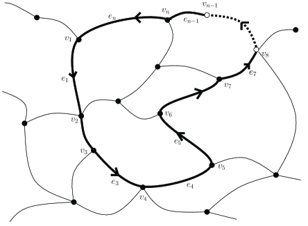
Figure 1: The loop ${\mathcal{L}}=\{e_{1},e_{2},..,e_{n}\}$ on the graph $\Gamma$.

Or, if instead of factorizing this expression by edges, we group the terms by vertices, we obtain:

$${\mathrm{T}r}\,G_{\mathcal{L}}\,=\,\sum_{r_{i}=0,1}(-1)^{\sum_{i}r_{i}}\frac{\prod_{i}\langle\varsigma^{r_{i-1}}z_{v_{i},e_{i-1}}\,|\,\varsigma^{1-r_{i}}z_{v_{i},e_{i}}\rangle}{\prod_{i}\sqrt{\langle z_{v_{i},e_{i-1}}|z_{v_{i},e_{i-1}}\rangle\langle z_{v_{i},e_{i}}|z_{v_{i},e_{i}}\rangle}},$$

where the $\varsigma^{r_{i}}$ records whether we have the term $|z_{v_{i},e_{i}}]\langle z_{v_{i+1},e_{i}}|$ or $|z_{v_{i},e_{i}}\rangle[z_{v_{i+1},e_{i}}|$ on the edge $e_{i}$, with $r_{i}=0,1$ (recall that $\varsigma$ is the anti-unitary map sending a spinor $|z\rangle$ to each dual $|z]$).

Depending on the specific values of the $r_{i}$ parameters, the scalar products at the numerators are given by the matrix elements of $M^{i}$ or $Q^{i}$ at the vertex $i$. Since these matrices are by definition $\mathrm{SU}(2)$-invariant (they commute with the closure conditions), this is a consistency check, a posteriori, that the holonomy ${\mathrm{T}r}\,G_{\mathcal{L}}$ correctly provides a $\mathrm{SU}(2)$-invariant observable.

Taking into account the various possibilities for the signs $(-1)^{r_{i}}$, we can write the holonomy

$${\mathrm{T}r}\,G_{\mathcal{L}}\,=\,\sum_{r_{i}=0,1}(-1)^{\sum_{i}r_{i}}\frac{{\mathcal{M}}_{\mathcal{L}}^{\{r_{i}\}}}{\prod_{i}\sqrt{\langle z_{v_{i},e_{i}}|z_{v_{i+1},e_{i}}\rangle}},$$ (30)

where the objects ${\mathcal{M}}_{\mathcal{L}}^{\{r_{i}\}}$ correspond to each term with a fixed set $\{r_{i}\}$:

$${\mathcal{M}}_{\mathcal{L}}^{\{r_{i}\}} \equiv \!\prod_{i}r_{i-1}r_{i}\bar{Q}^{i}_{i,i-1}+(1-r_{i-1})r_{i}M^{i}_{i-1,i}+r_{i-1}(1-r_{i})M^{i}_{i,i-1}+(1-r_{i-1})(1-r_{i})Q^{i}_{i,i-1}$$

$$= \!\prod_{i}\langle\varsigma^{r_{i-1}}z_{v_{i},e_{i-1}}\,|\,\varsigma^{1-r_{i}}z_{v_{i},e_{i}}\rangle.$$

Using these ingredients, we are going to write an action principle for this formalism. For this, we have to keep in mind the graph structure, with intertwiners at the vertices, glued together along edges. The phase space therefore consists of spinors $z_{v,e}$ (where $e$ are edges attached to the vertex $v$, i.e., such that $v=s(e)$ or $v=t(e)$) which we constrain by the closure conditions $\vec{{\cal C}}^{v}$ at each vertex $v$ and the matching conditions on each edge $e$. The corresponding action thus reads:

$$S_{0}^{\Gamma}[z_{v,e}]=\!\!\int\!\!dt\,\sum_{v}\sum_{e|v\in\partial e}\!\!\!\left(-i\langle z_{v,e}|\partial_{t}z_{v,e}\rangle+\langle z_{v,e}|\Lambda_{v}|z_{v,e}\rangle\right)\!+\sum_{e}\rho_{e}\!\left(\!\langle z_{s(e),e}|z_{s(e),e}\rangle\!\!-\!\!\langle z_{t(e),e}|z_{t(e),e}\rangle\!\right)\!,$$

where the $2\times 2$ Lagrange multipliers $\Lambda_{v}$, satisfying ${\mathrm{T}r}\,\Lambda_{v}=0$, impose the closure constraints and the Lagrange multipliers $\rho_{e}\in{\mathbb{R}}$ impose the matching conditions. All the constraints are first class, they generate $\mathrm{SU}(2)$ transformations at each vertex and $\mathrm{U}(1)$ transformations on each edge $e$.

Analogously, this system can be parameterized in terms of $N_{v}\times N_{v}$ unitary matrices $U^{v}$ and the parameters $\lambda_{v}$. The matrix elements $U^{v}_{ef}$ refer to pairs of edges $e,f$ attached to the vertex $v$. As mentioned before, the closure constraints are automatically encoded in the requirement of unitarity for $U^{v}$. It remains, then, to impose the matching conditions $M^{s(e)}_{ee}-M^{t(e)}_{ee}=0$ on each edge $e$ (the matrices $M^{v}=\lambda_{v}\,U^{v}\Delta(U^{v})^{-1}$ being functions of both $\lambda_{v}$ and $U^{v}$). So in this case, the action reads:

$$S_{0}^{\Gamma}[\lambda_{v},U^{v}]\,=\,\int dt\,\sum_{v}\left(-i\,\lambda_{v}{\mathrm{T}r}\,U^{v}\Delta\partial_{t}{U^{v}}^{\dagger}\,-\,{\mathrm{T}r}\Theta_{v}\,(U^{v}{U^{v}}^{\dagger}-\mathbb{I})\right)+\sum_{e}\rho_{e}(M^{s(e)}_{ee}-M^{t(e)}_{ee}),$$

where the $\rho_{e}$ impose the matching conditions while the $N_{v}\times N_{v}$ matrices $\Theta_{v}$ are the Lagrange multipliers for the unitarity of the matrices $U^{v}$.

This free action describes the classical kinematics of spin networks on the graph $\Gamma$. We can now add interaction terms to this action. Such interaction terms should be built with generalized holonomy observables ${\mathcal{M}}_{\mathcal{L}}^{\{r_{i}\}}$, thus trivially satisfying the closure and matching conditions. A proposal for a classical action for spin networks with non-trivial dynamics was made in [6]:

$$S_{\gamma_{\mathcal{L}}^{\{r_{i}\}}}^{\Gamma}=S_{0}^{\Gamma}\,+\,\int dt\,\sum_{{\mathcal{L}},\{r_{i}\}}\gamma_{\mathcal{L}}^{\{r_{i}\}}\,{\mathcal{M}}_{\mathcal{L}}^{\{r_{i}\}},$$

where the $\gamma_{\mathcal{L}}^{\{r_{i}\}}$ are the coupling constants giving the relative weight of each generalized holonomy in the full Hamiltonian. This action was then applied in particular to a specific model based on a 2-vertex graph. We refer the reader to the original paper for more details on the analysis of the dynamics derived from this Hamiltonian.

6 Spinor representation and Holomorphic methods in LQG

There is an interesting twist in the utility of this spinorial framework for LQG [3]. These methods are extremely powerful in order to understand the geometrical interpretation of the spin network states. The single-edge Hilbert space in LQG is given by $\mathcal{H}_{e}:=L^{2}(\mathrm{SU}(2),dg)$, i.e., the space of square integrable functions over the group $\mathrm{SU}(2)$. This Hilbert space can be obtained as the quantization of a cotangent bundle over $\mathrm{SU}(2)$ acting as the classical phase space ($T^{*}\mathrm{SU}(2)\approx\mathrm{SU}(2)\times{\mathfrak{s}u}(2)$). At this point, instead of the usual coordinatization of this classical phase space given by $(g,X)$ –a group and a Lie algebra element respectively–, a pair of $\mathbb{C}^{2}$-spinors $(|z\rangle,|\tilde{z}\rangle)$ recovering the classical physics in $T^{*}\mathrm{SU}(2)$ can be employed.

As we have already seen before it is possible to obtain the $\mathrm{SU}(2)$ group elements associated to such a pair of spinors. We are going to review that discussion simplifying the notation and taking a slightly different choice of mapping between the spinors and the group element and its inverse. We start with spinors $|z\rangle$ and $|\tilde{z}\rangle$, living at the source and the target vertices of a given edge, then we can write the corresponding $\mathrm{SU}(2)$-element and its inverse as follows:

$$g(z,\tilde{z}) = \dfrac{|z\rangle[\tilde{z}|-|z]\langle\tilde{z}|}{\|z\|\,\|\tilde{z}\|}\,,$$

$$g^{-1}(z,\tilde{z}) = \dfrac{-|\tilde{z}\rangle[z|+|\tilde{z}]\langle z|}{\|z\|\,\|\tilde{z}\|}\,.$$

It is straightforward to show that, under a local $\mathrm{SU}(2)$-transformation $h\in\mathrm{SU}(2)$ in the defining representation of the group, $g(z,\tilde{z})$ transforms as the holonomy of a $\mathrm{SU}(2)$-connection:

$$g(z,\tilde{z})\longmapsto h_{1}g(z,\tilde{z})h_{2}^{-1}\,.$$

Moreover, each spinor is mapped to $\mathbb{R}^{3}$ (up to a phase) yielding area vectors corresponding to the different faces of an elementary polyhedron. In this sense, the Hilbert space for a graph with $E$ edges can be regarded as the space of glued polyhedra covering a piecewise flat manifold (this is ensured by the imposition of the proper matching conditions). Following this line of thought, it is easy to show that the ${\mathfrak{s}u}(2)$-elements $X(z):=\vec{X}(z)\cdot\vec{\sigma}$ and $\tilde{X}(\tilde{z}):=\vec{\tilde{X}}(\tilde{z})\cdot\vec{\sigma}$, associated with the normals to the glued faces of two polyhedra, are related through the expression:

$$\tilde{X}=g^{-1}Xg.$$

On the other hand, we can endow the space $\mathbb{C}^{2}\times\mathbb{C}^{2}$ with a symplectic structure given by

$$\{\bar{z}^{i},z^{j}\}=i\delta_{i}^{j}=\{\bar{\tilde{z}}^{i},\tilde{z}^{j}\}\,,$$

thus obtaining a proper phase space. This phase space has to be equipped with a constraint forcing the two spinors to have the same length (matching condition). This constraint is given by $\|z^{2}\|-\|\tilde{z}^{2}\|$ and it can be noticed that it generates $\mathrm{U}(1)$ transformations. Nevertheless, the group and Lie-algebra elements are invariant under these transformations by construction. The interesting point here is that, using this symmetry, one can arrive to the cotangent bundle of $\mathrm{SU}(2)$ by means of a $\mathrm{U}(1)$-gauge reduction:

$$\mathbb{C}^{2}\times\mathbb{C}^{2}/\!\!/\mathrm{U}(1)/\mathbb{Z}_{2}\simeq T^{*}\mathrm{SU}(2)\setminus\{|X|=0\}\,,$$

where $/\!\!/$ denotes a double quotient (see [3] for details). This space has indeed the correct symplectic structure –that arises in terms of $g$ and $X$– written in terms of spinors. In this sense, given an edge of a graph, one can either assign it a pair $(g,X)$ or a pair of spinors $(|z\rangle$, $|\tilde{z}\rangle)$. This way, the degrees of freedom are shifted from the edge to its vertices.

Once we are convinced that this correspondence between spinors and the $\mathrm{SU}(2)$-group and algebra elements works, we can also find the expression of the Haar measure $dg$ in terms of spinors. The result is really simple, the Haar measure is just the product of two Gaussian measures

$$\int_{\mathrm{SU}(2)}dg=\int_{\mathbb{C}^{2}\times\mathbb{C}^{2}}d\mu(z)d\mu(\tilde{z}).$$

In order to arrive to this result one has to be careful with the redundancies introduced by the spinors ($8$ degrees of freedom instead of the $3$ in a group element $g$) which means that one has to make use of a twisted rotation (as defined in [3]) in order to implement a $\mathrm{SU}(2)$-transformation leaving the group element invariant. Taking this into account the former relation can be proven by computing the scalar product between two representation matrices of $\mathrm{SU}(2)$ in terms of spinors. We refer the interested reader to the original paper for more details.

The procedure presented here provides an alternative quantization for $T^{*}\mathrm{SU}(2)$, where the Hilbert space for an edge $e$, $\mathcal{H}^{spin}_{e}$ is obtained after an appropriate gauge-reduction, implementing the proper matching conditions on that edge, of the Bargmann space of holomorphic square-integrable functions on both spinors. This is, in some sense, an opposite way of thinking with respect to the usual picture, where the group and Lie algebra elements are taken as the fundamental variables. Here, the spinorial variables are considered as fundamental and the group and Lie algebra elements arise as composite objects. We can also build ladder operators in terms of spinors and derive the standard holonomy and flux-operators of the theory.

We are considering two quantizations of the same classical phase space, resulting from the use of two different polarizations, and we arrive at the usual LQG Hilbert space $\mathcal{H}_{e}$ with the standard variables or to $\mathcal{H}^{spin}_{e}$ in terms of spinors. The relevant question then is, are those Hilbert spaces unitarily equivalent? The answer is in the affirmative. Indeed, one can construct a unitary map between those Hilbert spaces

$$\mathcal{T}:\mathcal{H}_{e}\rightarrow\mathcal{H}_{e}^{spin}$$

employing a method based on a modification of the Segal-Bargmann transform. This map sends $SU(2)$ representation matrices to holomorphic functions in $(|z\rangle,|\tilde{z}\rangle)$ and it can be regarded as the restriction to the holomorphic part of the group element written in terms of spinors (see [3] for details). Furthermore, this map can be straightforwardly generalized to an arbitrary graph and can be shown to be compatible with the inductive limit construction used to define the Hilbert space of the continuum theory. Therefore, there is a strong formal consistency for this reformulation of LQG, which captures the same physics while opening new ways to tackle the open problems in the theory, such as the lack of a well defined semiclassical limit or the geometric interpretation of the spin networks states.

7 Conclusions

We have reviewed here the $\mathrm{U}(N)$ and spinorial framework for LQG. This new point of view has become a very useful tool to deal with certain fundamental problems in LQG. In particular, it was interesting for the study of a simple model (the $2$-vertex model) with a pair of nodes and an arbitrary number of links [5, 6, 9]. In these papers, a plausible dynamics was proposed for this system (at the quantum and classical level) and some striking mathematical analogies with loop quantum cosmology were explored. Also, using this framework, it was possible to study semiclassical states [4] and the simplicity constraints [10].

Let us revisit the main points presented in this review:

• Making use of the Schwinger representation, it is possible to write $\mathrm{SU}(2)$ invariant operators acting on the Hilbert space of intertwiners in LQG [1].

• A key point for the $\mathrm{U}(N)$ construction is that the LQG Hilbert space of intertwiners with $N$-legs and fixed total area $J$ carries an irreducible $\mathrm{U}(N)$ representation [2].

• One can show that the full space of $N$-leg intertwiners is endowed with a Fock space structure, with annihilation and creation operators given by the operators $F_{ij}$ and $F_{ij}^{\dagger}$.

• We have presented a classical framework based on spinors whose quantization (using holomorphic methods) leads back to the $\mathrm{U}(N)$ framework for the Hilbert space of intertwiners in LQG [6].

• An action principle for the spinor phase space has been described. Then, using the relation given in [8] between spinors and $\mathrm{SU}(2)$ group elements, an expression for the holonomy operators was built. Taking advantage of these $\mathrm{SU}(2)$ and $\mathrm{U}(1)$ invariant operators, it was possible to give a generic interaction term (whose quantization is direct) for this framework.

• Finally, we gave a glimpse of the formal and rigorous construction of the spinor representation and holomorphic quantization techniques for the whole LQG kinematical Hilbert space, as it was developed by Livine and Tambornino [3]. There, it was shown that although the choice of the spinors as fundamental variables of the theory implies a different choice of polarization (and in general different polarizations lead to inequivalent quantizations), in this case it is possible to construct explicitly a unitary map $\mathcal{T}$ between the usual LQG Hilbert space and the one derived in terms of the spinors.

Both the $\mathrm{U}(N)$ framework and the spinor representation are promising ways to deal with the most important open problems within LQG, namely, the semiclassical states and the dynamics. They may also become useful computational tools to calculate physical quantities within the theory, such as correlation functions. Besides, this new point of view may be useful in the context of group field theory. The possibility of having Feynman amplitudes expressed as integrals over spinor variables or the study of the renormalization properties of group field theories are interesting problems where the spinor representation can play a crucial role.

To conclude, we would like to remark that this framework certainly constitutes a viewpoint that opens new ways of research, both in loop quantum gravity and in group field theory and spin foams, that are worth exploring.

Acknowledgements

We would like to thank Etera R. Livine for endless discussions.

This work was in part supported by the Spanish MICINN research grants FIS2008-01980, FIS2009-11893 and ESP2007-66542-C04-01 and by the grant NSF-PHY-0968871. IG is supported by the Department of Education of the Basque Government under the “Formación de Investigadores” program.

References

• [1] Florian Girelli and EteraΒ R. Livine. Reconstructing quantum geometry from quantum information: Spin networks as harmonic oscillators. Class.Quant.Grav. 22 (2005) 3295-3314 [arXiv:gr-qc/0501075].
• [2] Laurent Freidel and EteraΒ R. Livine. The Fine Structure of $\mathrm{SU}(2)$ Intertwiners from $\mathrm{U}(N)$ Representations. J.Math.Phys. 51 (2010) 082502 [arXiv:0911.3553v1].
• [3] EteraΒ R. Livine and Johannes Tambornino. Spinor Representation for Loop Quantum Gravity. [arXiv:1105.3385v1].
• [4] Laurent Freidel and EteraΒ R. Livine. $\mathrm{U}(N)$ Coherent States for Loop Quantum Gravity. J.Math.Phys. 52 (2011) 052502 [arXiv:1005.2090v1].
• [5] EnriqueΒ F. Borja, Jacobo Diaz-Polo, IΓ±aki Garay and EteraΒ R. Livine. Dynamics for a 2-vertex Quantum Gravity Model. Class.Quant.Grav. 27 (2010) 235010 [arXiv:1006.2451v2].
• [6] EnriqueΒ F. Borja, Laurent Freidel, IΓ±aki Garay and EteraΒ R. Livine. $\mathrm{U}(N)$ tools for Loop Quantum Gravity: The Return of the Spinor. Class.Quant.Grav. 28 (2011) 055005 [arXiv:1010.5451v1].
• [7] Laurent Freidel and Simone Speziale. Twisted geometries: A geometric parametrisation of $\mathrm{SU}(2)$ phase space. Phys. Rev. D82 (2010) 084040 [arXiv:1001.2748v3].
• [8] Laurent Freidel and Simone Speziale. From twistors to twisted geometries. Phys. Rev. D82 (2010) 084041 [arXiv:1006.0199v1].
• [9] EnriqueΒ F. Borja, Jacobo Diaz-Polo, IΓ±aki Garay and EteraΒ R. Livine. $\mathrm{U}(N)$ invariant dynamics for a simplified Loop Quantum Gravity model. [arXiv:1012.3832v1].
• [10] Maite Dupuis and EteraΒ R. Livine. Revisiting the Simplicity Constraints and Coherent Intertwiners. Class.Quant.Grav. 28 (2011) 085001 [arXiv:1006.5666v1].