Tidal dissipation in multi-planet systems and constraints to orbit-fitting

Abstract

Context. We present here in full details the linear secular theory with tidal damping that was used to constraint the fit of the HD10180 planetary system in (Lovis et al., 2011). The theory is very general and can provide some intuitive understanding of the final state of a planetary system when one or more planets are close to their central star. We globally recover the results of (Mardling, 2007), but we show that in the HD209458 planetary system, the consideration of the tides raised by the central star on the planet lead to believe that the eccentricity of HD209458b is most probably much smaller than $0.01$.

Aims.

Methods.

Results.

1 Introduction

In several planetary systems, some planets are very close to their central star and thus subject to strong tidal interaction. If a planet were alone around its star, this will led to a circularization of its orbit. However, for multi-planet system, due to the secular interaction between the planets, the final evolution of the system may be different, with residual eccentricity (Wu & Goldreich, 2002; Mardling, 2007; Batygin et al., 2009; Mardling, 2010; Lovis et al., 2011). This is also why fitting a circular orbit to the innermost planets in a system subject to tidal dissipation will not insure that its eccentricity remains small, as the secular interactions may drive it to large values (Lovis et al., 2011). One thus needs to take into account the fact that the observed system is the result of a tidal process (Lovis et al., 2011). Here, we develop in full details the method that has been used in (Lovis et al., 2011) for the fit to a tidally evolved system. The theory is very general and is compared to previous results of (Mardling, 2007, 2010).

2 Model

2.1 Newtonian interaction

Without mean-motion resonances, the long term evolution of a conservative multiplanetary system is given, in first order, by the Laplace-Lagrange linear secular equations (see Laskar, 1990). With this approximation, inclinations and eccentricities are decoupled and follow the same kind of evolution. For simplicity, in this letter we will focus only on coplanar systems. Let $n$ be the number of planets. Using the classical complex variables $z_{k}=e_{k}{\rm e}^{{\rm i}\varpi_{k}}$, $k=1,\ldots,n$, where $e_{k}$ and $\varpi_{k}$ are respectively the eccentricity and the longitude of the periastron of the $k$-th planet, the secular equations read

$$\frac{d}{dt}[z]={\rm i}A\,[z]\ ,\qquad\hbox{with}\quad[z]=\left(\begin{array}[]{c}z_{1}\\ \vdots\\ z_{n}\end{array}\right)\ ,$$ (1)

and where $A$ is a real matrix whose elements are (Laskar & Robutel, 1995)

$${\displaystyle A_{jj}}$$

(2)

In these expressions, $m_{k}$ and $a_{k}$, are the mass and semi-major axis of the $k$-th planet, while the mean motion $n_{k}$ is defined by $n_{k}^{2}a_{k}^{3}=G(m_{0}+m_{k})$. By assumption, planets are ordered by increasing semi-major axis while the index 0 stands for the star. The functions $C_{2}(\alpha)$ and $C_{3}(\alpha)$ are defined by mean of ${\rm b}_{s}^{(k)}$, the usual Laplace coefficients (e.g. Laskar & Robutel, 1995), as:

$${\displaystyle C_{2}(\alpha)}$$

(3)

2.2 Other effects

The above secular equations (1) describe only the Newtonian interactions between point mass planets. In order to study exoplanetary systems with short period planets, it is often necessary to add corrections due to relativity, oblateness and tidal friction, at least to the inner planets. The spatial secular equations of motion resulting from all these effects are given in (Lambeck, 1980; Eggleton & Kiseleva-Eggleton, 2001; Ferraz-Mello et al., 2008). To first order in eccentricity, and in the planar case, they modify the diagonal terms of the matrix $A$ in two different ways. There are conservative terms that are purely imaginary, and dissipative ones which are real (and negative). We thus define two new diagonal matrices $\delta A=\sum_{i=1,5}\delta A^{(i)}$ and $\delta B=\sum_{i=4,5}\delta B^{(i)}$ such that the full secular evolution is given by

$$\frac{d}{dt}[z]=({\rm i}{{A_{\rm tot}}}-{\delta B})[z]\ ,$$ (4)

with ${{A_{\rm tot}}}=A+{\delta A}$. The effect of relativity on the $k$-th planet is conservative, and in first order in eccentricity, it leads to

$$\delta A^{(1)}_{kk}=3\frac{Gm_{0}}{c^{2}}\frac{n_{k}}{a_{k}}\ .$$ (5)

The effect of the oblateness of bodies generated by their proper rotation are

$$\delta A^{(2)}_{kk}=\frac{k_{2,k}\,n_{k}}{2}\left(\frac{m_{0}+m_{k}}{m_{k}}\right)\left(\frac{R_{k}}{a_{k}}\right)^{5}\left(\frac{\omega_{k}}{n_{k}}\right)^{2}\ ,$$ (6)

and

$$\delta A^{(3)}_{kk}=\frac{k_{2,k}\,n_{k}}{2}\left(\frac{m_{0}+m_{k}}{m_{0}}\right)\left(\frac{R_{0}}{a_{k}}\right)^{5}\left(\frac{\omega_{0}}{n_{k}}\right)^{2}\ ,$$ (7)

for the oblateness of the $k$-th planet and the oblateness of the star. $k_{2,k}$, $\omega_{k}$, and $R_{k}$ are respectively the second Love number, the proper rotation rate, and the radius of the $k$-th body. Tidal effects have two contributions. With the same approximation, we have

$$\delta A^{(4)}_{kk}=\frac{15}{2}K_{k}\ ,\qquad\delta B^{(4)}_{kk}=27\left(1-\frac{11}{18}\frac{\omega_{k}}{n_{k}}\right)\frac{K_{k}}{Q_{k}}\ ,$$ (8)

with

$$K_{k}=k_{2,k}n_{k}\left(\frac{m_{0}}{m_{k}}\right)\left(\frac{R_{k}}{a_{k}}\right)^{5}$$ (9)

for the tides raised on the $k$-th planet by the star, and

$$\delta A^{(5)}_{kk}=\frac{15}{2}K^{\prime}_{k}\ ,\qquad\delta B^{(5)}_{kk}=27\left(1-\frac{11}{18}\frac{\omega_{0}}{n_{k}}\right)\frac{K^{\prime}_{k}}{Q_{0}}\ ,$$ (10)

with

$$K^{\prime}_{k}=k_{2,0}n_{k}\left(\frac{m_{k}}{m_{0}}\right)\left(\frac{R_{0}}{a_{k}}\right)^{5}$$ (11)

for the tides raised on the star by the $k$-th planet. We consider here the “viscous” approach (Singer, 1968; Mignard, 1979), where the quality factor of the $k$-th body is $Q_{k}\equiv(n_{k}(\Delta t)_{k})^{-1}$ and $(\Delta t)_{k}$ is a constant time lag.

3 Resolution

3.1 Conservative case

When there is no dissipation ($\delta B=0$) the system is classically resolved by diagonalizing the matrix ${{A_{\rm tot}}}$ through a linear transformation

$$[z]=S_{0}[u]\ .$$ (12)

In the new variables, the equations of motion become

$$\frac{d}{dt}[u]={\rm i}D_{0}[u]\ ,\quad\hbox{where}\quad D_{0}=S_{0}^{-1}{{A_{\rm tot}}}S_{0}$$ (13)

is the diagonal matrix ${\rm diag}(g_{1},\ldots,g_{n})$ of the eigenvalues $g_{k}$ of ${{A_{\rm tot}}}$. We have then

$$u_{k}(t)=u_{k}(0){\rm e}^{{\rm i}\,g_{k}t}\ .$$ (14)

Each proper mode $u_{k}$ describes a circle in the complex plane at a constant frequency $g_{k}$ and with the radius $\left|u_{k}(0)\right|$. The evolution of the planetary eccentricities are then given by (12). They are linear combinations of the proper modes.

The only differences between $A$ and ${{A_{\rm tot}}}$ are in the diagonal terms. Those of ${{A_{\rm tot}}}$ are larger or equal to those of $A$. As a consequence, using ${{A_{\rm tot}}}$ instead of $A$ makes the fundamental frequencies $g_{k}$ larger and the coupling between the proper modes lower (the evolution of the eccentricity of each planet is almost given by one single proper mode, the other modes generate only small oscillations).

3.2 General solution

In the full linear secular equation (4), the matrix that has to be diagonalized is now ${\rm i}{{A_{\rm tot}}}-{\delta B}$, where the dissipation part ${\delta B}$ comes only from tides. In general, the elements of ${\delta B}$ are much smaller than those of the diagonal of ${{A_{\rm tot}}}$. ${\delta B}$ will thus be considered as a perturbation of the conservative evolution given by ${{A_{\rm tot}}}$. Let

$$S=S_{0}({{1}}+{\rm i}\delta S_{1})\ ,$$ (15)

be the matrix of the linear transformation that diagonalizes the full system. As ${\delta B}$ is a perturbation of ${{A_{\rm tot}}}$, we will make the hypothesis that the matrix ${\delta S}_{1}$ is also a perturbation of the matrix $S_{0}$. At first order, the inverse of $S$ is

$$S^{-1}=({{1}}-{\rm i}{\delta S}_{1})S_{0}^{-1}\ ,$$ (16)

and the new diagonal matrix is $D=iD_{0}-{\delta D}_{1}$, with

$${\delta D}_{1}=S_{0}^{-1}({\delta B})S_{0}-[{\delta S}_{1},D_{0}]\ ,$$ (17)

where the bracket is defined by $[{\delta S}_{1},D_{0}]={\delta S}_{1}D_{0}-D_{0}{\delta S}_{1}$. For ${\delta D}_{1}$ to be actually diagonal, ${\delta S}_{1}$ is given by

$$({\delta S}_{1})_{jk}=\frac{1}{g_{k}-g_{j}}\big{(}S_{0}^{-1}({\delta B})S_{0}\big{)}_{jk}\ ,\qquad j\neq k\ .$$ (18)

As $D_{0}$ is diagonal, all terms in the diagonal of $[{\delta S}_{1},D_{0}]$ vanish. Thus, the diagonal terms of ${\delta S}_{1}$ do not appear in the computation of ${\delta D}_{1}$ (17) and they can be set equal to zero. Let ${\delta D}_{1}={\rm diag}(\gamma_{1},\ldots,\gamma_{n})$. From (17), we have then

$$\gamma_{k}=\big{(}S_{0}^{-1}({\delta B})S_{0}\big{)}_{kk}\ .$$ (19)

These $\gamma_{k}$ are real and positive. It turns out that the imaginary part of $D$ is still the one of the conservative case $D_{0}$ (13). The proper frequencies $g_{k}$ are not affected by the dissipation ${\delta B}$. However, each proper mode now contains a damping factor $\gamma_{k}$ given by (19). The equations of motion in the new variables now read

$$\frac{d}{dt}[u]={\rm diag}({\rm i}g_{1}-\gamma_{1},\ldots,{\rm i}g_{n}-\gamma_{n})[u]\ ,$$ (20)

and the solutions are

$$u_{k}(t)=u_{k}(0){\rm e}^{-\gamma_{k}t}{\rm e}^{{\rm i}g_{k}t}\ .$$ (21)

It should be stressed that even if only one planet undergoes tidal dissipation (only $(\delta B)_{11}$ is different from 0 for example), because of the linear transformation $S_{0}$, all the eigenmodes can be damped (19).

4 Two planet case

In a simpler two planet system where only the first one undergoes tidal friction, ${\delta B}={\rm diag}(\gamma,0)$, the two proper frequencies are given by

$${\displaystyle g_{1}}$$

(22)

where $T$ and $\Delta$ are the trace and determinant of $A_{tot}$. From (19), it can be shown that the two dissipation factors are

$${\displaystyle\gamma_{1}}$$

(23)

The sum $\gamma_{1}+\gamma_{2}$ is equal to $\gamma$. There is thus always one eigenmode damped in a timescale shorter than $2\gamma^{-1}$ while the other is damped in a timescale larger than $2\gamma^{-1}$. In the particular case where $A_{11}=A_{22}$, we have $\gamma_{1}=\gamma_{2}=\gamma/2$.

Once the first eigenmode is damped, the ratio between the two eccentricities and the difference between the two longitudes of periastron are deduced from (12). We have

$${\displaystyle\frac{e_{1}}{e_{2}}}$$

(24)

It should be noted that the matrix ${\delta S}_{1}$ introduces small corrections in the difference between the longitudes of periastron which are not taken into account in (24).

Figure 1: Tidal effects on the eccentricity of HD 209458b with one or 2 companions. (a) The companion is a $0.1M_{J}$ planet at 0.4 AU with $e_{2}=0.4$ as in (Mardling, 2007). The blue curve has been obtained without considering the conservative effect of the tides (${\delta A}^{(4)}_{11}$ in eq. 8). The red curve in (a), and all the evolutions in the subfigures (b), (c), and (d) take into account this effect. (b) The mass of the companion is set to $0.608M_{J}$ in order to recover the final excentricity of Mardling’s simulation. The red curve is the result of a numerical integration of the full secular equations exact in eccentricity. The green one is the analytical solution of the linearized problem. (c) Same as (b) except for the initial $Q$-value of HD 209458b which is set to 15.15 to enable the visualisation of both the damping and the oscillation of the eccentricity. (d) Same as (c) with an additional $0.1M_{J}$ companion at 1.0 AU with $e_{3}=0.1$.

Figure 2: Eccentricity $e_{2}$ of the hypothetical companion of HD 209458b with $e_{1}=0.01$ assuming that the eigenmode with the shortest dissipation timescale is damped (black curves in panel a) and b)). a) The mass of the companion is fixed to $m_{2}=0.2M_{J}$. Negative values of $e_{2}$ correspond to $\Delta\varpi=180\deg$ while positive ones mean $\Delta\varpi=0\deg$. The dotted line is the eccentricity that the companion would have had 5.5 Gyr ago assuming a dissipation factor computed with (23). b) Same as a) for different masses $m_{2}$ while the semi-major axis is fixed and set to $a_{2}=0.4$ AU. c) Stellar reflex velocity due to the companion at periastron with the eccentricity of the figure a). d) idem for the eccentricity of the figure b). In grey regions, the eccentricity of the companion should have been larger than 1 in the past. The configuration appearing in all panels with the same orbital parameters is marked by a fill circle.

5 Application to HD 209458b

Here we compare the results of this paper with those of Mardling (2007) on the example of HD 209458b (Table 1). As in (Mardling, 2007), we first assume that the non zero eccentricity of this planet is due to the presence of a $m_{2}=0.1M_{J}$ companion at $a_{2}=0.4$ AU with an eccentricity $e_{2}=0.4$. For this study, eccentricities are large and modify the frequencies $g_{k}$ given by the analytical expression of the matrix ${{A_{\rm tot}}}$ (4). Thus, we chose to compute the matrix ${{A_{\rm tot}}}$ using a frequency analysis on a numerical integration of the system without dissipation exact in eccentricity and expanded up to the 4 order in the ratio of the semi-major axes (e.g. Mardling & Lin, 2002; Laskar & Boué, 2010). At first order, the eccentricity variables $z_{1}$ and $z_{2}$ are linear combinations of two eigenmodes $u_{1}$ and $u_{2}$ (21)

$${\displaystyle z_{1}(t)}$$

(25)

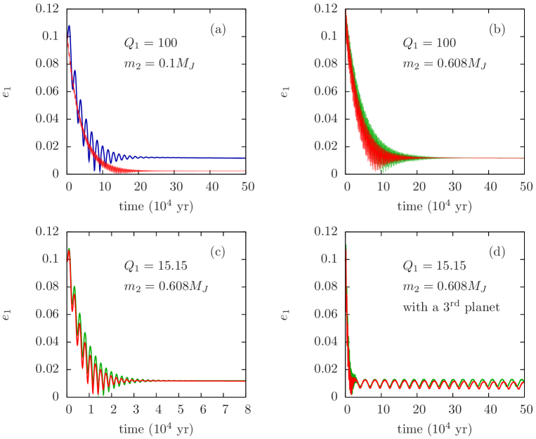
where $S$ is given by (15). With $Q_{1}=10^{5}$ and $\omega_{1}=n_{1}$, the two damping timescales (23) are $\gamma_{1}^{-1}\sim\gamma^{-1}=46$ Myr and $\gamma_{2}^{-1}=589$ Gyr. With an age estimate of 5.5 Gyr for this system (Burrows et al., 2007), the first eigenmode should be damped and the modulus of the second should remain almost constant. In consequence, both eccentricity variables should be proportional to $u_{2}$. Their modulus should thus be constant and verify (24), or equivalently, $e_{1}\approx e_{2}\,S_{12}/S_{22}=0.0025$. In (Mardling, 2007, Fig. 3), this value is larger, $e_{1}=0.012$. The difference comes from the tidal deformation of the planet that leads to the coefficient ${\delta A}^{(4)}_{11}$ in Eq. (8). This was not taken into account in (Mardling, 2007), and it accelerates the precession of the periapse of HD 209458b by a factor 6.6 (see Fig. 1a). In figure 1a, the initial $Q$-value of the planet is set artificialy to 100 to enable a direct comparison with the figure 3 of (Mardling, 2007). As said by Mardling (2007), and showed in this paper, the $Q$-value only affects the damping timescales but not the precession frequencies, nor the eccentricity amplitudes. However, with a larger precession frequency, the matrix ${{A_{\rm tot}}}$ is closer to a diagonal matrix. The two planets are less coupled and the ratio $S_{12}/S_{22}$ (25), equal to the final eccentricity ratio $e_{1}/e_{2}$, is smaller.

Table 1: Data for HD 209458b.

HD 209458b
Period (day)	3.5247
$m_{0}$ ($M_{\odot}$)	1.10
$m_{1}$ ($M_{J}$)	$0.64\pm 0.06$
$a_{1}$ (AU)	0.045
$e_{1}$	$0.014\pm 0.009$
$R_{1}$ ($R_{J}$)	$1.32\pm 0.03$

note: As in (Mardling, 2007), all parameters come from (Burrows et al., 2007) except the eccentricity that comes from (Laughlin et al., 2005).

One way to recover the final eccentricity of HD 209458b is to increase the mass of the companion up to $m_{2}=0.608M_{J}$ (Fig. 1b). Here, our aim is not to explain the large eccentricity of HD 209458b, but simply to illustrate the results of the section 3.2.

As the precession of the periastron of the inner planet is faster than in (Mardling, 2007, Fig. 3), we decreased the initial $Q$-value to 15.15 to accelerate the damping and to obtain an evolution with the same $g_{1}/\gamma_{1}$ ratio as in (Mardling, 2007) (Fig. 1c). As said before, this does not change the final eccentricity, but it illustrates better the damping of the first mode with frequency $g_{1}=0.14$ deg/yr.

After the damping of the first eigenmode, the eccentricities are not oscillating because there remains only one eigenmode with a non-zero amplitude. Both eccentricity variables $z_{1}$ and $z_{2}$ describe a circle in the complex plane at the same frequency $g_{2}$. But if a third planet is added to the system, a new eigenmode appears with a frequency $g_{3}$. Then eccentricities are oscillating (Fig. 1d). It should be noted that a relative inclination between planets can also generate an other eigenmode and make eccentricities oscillate (Mardling, 2010). However, in the linear approach eccentricities and inclinations are decoupled. It is thus necessary to have large eccentricities or inclinations to have significant oscillations.

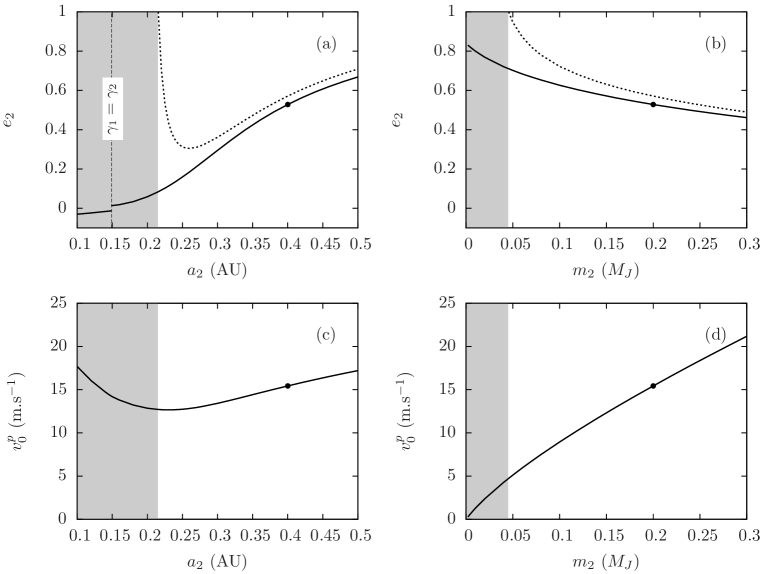
We now wonder which companion parameters can lead to an eccentricity $e_{1}=0.01$ for HD 209458b. As the system contains two planets, eccentricities are at most combination of two eigenmodes. But since $\gamma^{-1}=46$Myr is less than the age of the system (5.5 Gyr), at least one of the eigenmode is damped. However both eigenmodes cannot have zero amplitude, else the two orbits would be circular. Thus, let us assume that remains only a single eigenmode, the one with the longer damping timescale. Then, given a semi-major axis $a_{2}$ and a mass $m_{2}$, the eccentricity of the companion is obtained through (24) at first order. In practice we integrated numerically the system without dissipation, and found the eccentricity $e_{2}$ that cancels the amplitude of the rapidly damped eigenmode. Results are shown with solid curves in figure 2a and 2b. Once the current eccentricity $e_{2}$ is given, the initial value (5.5 Gyr ago) is estimated assuming an exponential decay with a damping factor given by (23) (see the dotted curves Fig. 2a and Fig. 2b). The frequencies $g_{k}$ and the coefficients $A_{kk}$ were obtained numerically using a frequency analysis. Parameters leading to initial eccentricities larger than 1 are excluded. They correspond to the grey regions in figure 2. Although planets are less coupled than in (Mardling, 2007), there is still a large range of initial conditions leading to a state compatible with $e_{1}=0.01$. However, the stellar reflex velocity due to the companion at periastron (Fig. 2c and 2d) is above the detectability threshold of about 3 m.s^-1. For example, with $a_{2}=0.25$ AU, and $m_{2}=0.05M_{J}$, the current eccentricity is $e_{2}=0.34$ and the maximal stellar reflex velocity $v_{0}^{p}=3.9$ m.s^-1. It thus seems that such a planet cannot exist. Indeed, observations do not constrain strongly the eccentricity of HD 209458b and a circular orbit is not ruled out (Laughlin et al., 2005).

6 Orbit fitting : the HD10180 case

Figure 3: Tidal evolution of the amplitude of the proper modes $\left|u_{1}\right|$ (red), $\left|u_{2}\right|$ (green), $\left|u_{3}\right|$ (blue), and $u_{4}$ (pink) resulting from the tidal dissipation on planet HD10180$b$ with $k_{2}/Q=0.0015$ (Lovis et al., 2011).

Figure 4: Evolution of the eccentricity of planet HD10180b over 250 kyr starting with $e_{b}=0$ at $t=0$ (present time) for three different models : In red, the numerical integration is purely Newtonian and do not take into account general relativity (GR). In green, GR is taken into account in the integration. In blue, GR is taken into account and the fit is made with the tidal dissipation constraint (26).

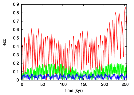
The analysis of the radial velocities measures of HD10180 revealed the potential existence of 7 planets in this system (Lovis et al., 2011). The innermost planet, HD10180b, is a terrestrial planet ($m_{b}\sin i=1.35M_{\oplus}$) with period of $\approx 1.177$ days and semi-major axis $a_{b}=0.0223$ AU. The planet is thus subject to strong tidal interaction with the central star. During the first fit (Lovis et al., 2011, Table 3) , it was thus assumed that its eccentricity has been damped to very small values, and its value was fixed to $e_{b}=0$. Nevertheless, if the system is then numerically integrated over 250 kyr (Fig. 4 (red curve)), due to secular interactions with the other planets, $e_{b}$ grows very rapidly to high values, reaching nearly 0.9.

When general relativity (GR) is included in the numerical integration, the main effect is to increase the diagonal terms of the secular matrix (Eq.5). As a result, the secular variations of $e_{b}$ are much smaller (Fig. 4 (green curve)), but still reach $0.2$.

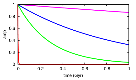
The strategy that was adopted for the final fit of (Lovis et al., 2011) was to include in the fit the constraint that the planetary system that is searched for is the result of the tidal evolution, as described in section 3.2. As the planet has a mass comparable to the Earth, it can be assumed to be terrestrial, and thus to have a dissipation factor of the same order of magnitude as (or larger than) Mars $k_{2}/Q=0.0015$, which is the smallest value among the terrestrial planets in the Solar System. The damping factors ${\rm e}^{-\gamma_{k}}\,t$ can thus be computed through (Eq. 19) for all proper modes $u_{k}$ (Lovis et al., 2011, Table 5). The resulting dampings of the amplitudes of the proper modes $u_{k}$ are given in Fig.3.

From this computation, as the age of the system is estimated to be of about 4 Gyr, it can be seen that the first two proper modes amplitudes $u_{1}$ and $u_{2}$ are certainly reduced to very small values. If the damping factor $k_{2}/Q$ were 10 times smaller, the conclusion would be nearly the same, as the only change in Fig.3 would be a change in the time scale of the figure, the units being now 10 Gyr instead of 1 Gyr.

In order to include the constraint on the tidal damping in the fit, one can then add to the $\chi^{2}$ minimization the additional term

$$\chi^{2}_{R}=R(\left|u_{1}\right|^{2}+\left|u_{2}\right|^{2})$$ (26)

where $R$ is an empirical constant that needs to be set to a value that will equilibrate the additional constraint with respect to the value of the $\chi^{2}$ in absence of constraint. After various trials, $R=350$ was used in (Lovis et al., 2011).

The computation of the amplitude of the proper modes $\left|u_{k}\right|$ during the fit is made iteratively. Once a first orbital solution is obtained, the Laplace-Lagrange linear system (Eq.1) is computed and thus also the matrix $S_{0}$ of transformation to proper modes (Eq.12). For a given initial condition $(z_{k})$ obtained through the fit, the proper modes $u_{k}$ are computed with

$$[u]=S_{0}^{-1}[z]$$ (27)

and the additional contribution (26) can then be computed in the fitting process. Practically, in an iterative fit taking into account the Newtonian interactions, the transformation matrix $S_{0}^{-1}$ just needs to be computed once, or twice if one wants to recompute the $S_{0}^{-1}$ matrix when the convergence to a final solution is obtained. In (Lovis et al., 2011), the final values were $u_{1}=0.0017$, $u_{2}=0.044$ for $R=350$, with a final $\sqrt{\chi^{2}}=1.24$, very close to the residuals obtained in absence of constraint ( $\sqrt{\chi^{2}}=1.22$).

In this constrained solution, the initial value of $e_{b}$ is still $0$, but the secular change due to planetary interactions is much smaller (Fig.4 (blue curve)), which ensure a more stable behavior to the system.

7 Conclusion

We have presented here in full details the secular theory with tidal dissipation that was outlined in (Lovis et al., 2011) for the system HD10180. The use of Lagrange-Laplace linear theory can include very easily the linear contribution due to tidal dissipation and provide an intuitive background for studying multi-planetary systems when one or several planets are close to their central star and subject to tidal damping. Although we have limited here the study to the planar case, this formalism can be easily extended to mutually inclined systems.

For the system HD209458, we could retrieve globally the results of (Mardling, 2007), although we find that a companion with mass $m_{2}=0.1M_{J}$ with $a_{2}=0.4$ AU and $e_{2}=0.4$ will not lead to $e_{1}=0.012$, but to a much smaller value of $e_{1}=0.0025$. This is due to the additional tides raised by the star on the planet $\delta A_{11}^{(4)}$ (Eq.8) in the contribution to the secular equations (Eq.4).

We have examined other configuration that could lead to a final eccentricity $e_{1}\geq 0.01$ for HD209458b, but our conclusion is negative, as we found that a potential companion, large enough to lead to a final eccentricity $e_{1}\geq 0.01$ leads to sufficiently large stellar motion that it should have already been detected, assuming a detectability threshold of 3 m.s^-1. Our conclusion is thus that the most probable outcome is that the actual eccentricity of HD209458b has a much smaller value than $0.01$.

References

- Batygin et al. (2009) Batygin, K., Laughlin, G., Meschiari, S., et al. 2009, ApJ, 699, 23
- Burrows et al. (2007) Burrows, A., Hubeny, I., Budaj, J., & Hubbard, W. B. 2007, ApJ, 661, 502
- Eggleton & Kiseleva-Eggleton (2001) Eggleton, P. P. & Kiseleva-Eggleton, L. 2001, ApJ, 562, 1012
- Ferraz-Mello et al. (2008) Ferraz-Mello, S., Rodríguez, A., & Hussmann, H. 2008, Celestial Mechanics and Dynamical Astronomy, 101, 171
- Lambeck (1980) Lambeck, K. 1980, The Earth’s Variable Rotation: Geophysical Causes and Consequences (Cambridge University Press)
- Laskar (1990) Laskar, J. 1990, Icarus, 88, 266
- Laskar & Boué (2010) Laskar, J. & Boué, G. 2010, A&A, 522, 11
- Laskar & Robutel (1995) Laskar, J. & Robutel, P. 1995, Celestial Mechanics and Dynamical Astronomy, 62, 193
- Laughlin et al. (2005) Laughlin, G., Marcy, G. W., Vogt, S. S., Fischer, D. A., & Butler, R. P. 2005, ApJ, 629, L121
- Lovis et al. (2011) Lovis, C., Ségransan, D., Mayor, M., et al. 2011, A&A, 528, A112+
- Mardling (2007) Mardling, R. A. 2007, MNRAS, 382, 1768
- Mardling (2010) Mardling, R. A. 2010, MNRAS, 407, 1048
- Mardling & Lin (2002) Mardling, R. A. & Lin, D. N. C. 2002, ApJ, 573, 829
- Mignard (1979) Mignard, F. 1979, Moon and Planets, 20, 301
- Singer (1968) Singer, S. F. 1968, Geophys. J. R. Astron. Soc., 15, 205
- Wu & Goldreich (2002) Wu, Y. & Goldreich, P. 2002, ApJ, 564, 1024