Reconstructing the History of Energy Condition Violation from Observational Data

Abstract

We study the likelihood of energy condition violations in the history of the Universe. Our method is based on a set of functions that characterize energy condition violation. FLRW cosmological models are built around these “indication functions”. By computing the Fisher matrix of model parameters using type Ia supernova and Hubble parameter data, we extract the principal modes of these functions’ redshift evolution. These modes allow us to obtain general reconstructions of energy condition violation history independent of the dark energy model. We find that the data suggest a history of strong energy condition violation, but the null and dominant energy conditions are likely to be fulfilled. Implications for dark energy models are discussed.

1. Introduction

The energy conditions introduced by Hawking & Ellis (1973, Chapter 4) are coordinate-invariant inequality constraints on the energy-momentum tensor that appears in the Einstein field equation. They play an essential role in the proof of theorems in the general theory of relativity concerning the existence of spacetime singularities (see Wald 1984). Due to their simplicity and model-independence, the energy conditions are listed as one of many approaches to understand the evolution of universe.

Of the many proposed energy conditions, the ones we analyze in this paper are the null, the strong, and the dominant energy conditions (abbreviated respectively as NEC, SEC, and DEC). These energy conditions can be expressed as follows (Carroll 2004, Chapter 4) for a general stress-energy tensor $T$:

• NEC: $T_{\alpha\beta}n^{\alpha}n^{\beta}\geq 0$ for all null vectors $n$;

• DEC: $T_{\alpha\beta}t^{\alpha}t^{\beta}\geq 0$ and $T_{\alpha\beta}T^{\beta}_{\gamma}t^{\alpha}t^{\gamma}\leq 0$ for all timelike vectors $t$;

• SEC: $T_{\alpha\beta}t^{\alpha}t^{\beta}\geq\frac{1}{2}T^{\gamma}_{\gamma}t^{\delta}t_{\delta}$ for all timelike vectors $t$.

The energy conditions are of great relevancy to the study of cosmology. For example, the NEC is an important condition of stability for fluids (Dubovsky et al. 2006; Buniy et al. 2006), hence it is useful for the analysis of cosmological models. The DEC guarantees stability of a source obeying it and imposes on the dark energy equation of state parameter $w$ a lower bound $w\geq-1$ (Carroll et al. 2003). Violation of the $w\geq-1$ bound can lead to the “big rip doomsday” scenario of the Universe (Caldwell et al. 2003). It can also be shown that sudden future singularity solutions of the Friedmann-Lemaître-Robertson-Walker (FLRW) cosmology always violate the DEC (Lake 2004). Finally, SEC violation is a typical trait of a positive cosmological constant $\Lambda$ (for example, see Li et al. 2011) and other dark energy models (see Schuecker et al. 2003, and references therein). We therefore find an investigation of these energy conditions useful for our understanding of the Universe’s evolution.

The knowledge of cosmic energy condition violation has been greatly facilitated by precise observational data. Visser (1997a, b) shows that Hubble constant and stellar age measurements, which bound the age of the Universe, suggest a history of SEC violation (see also the review by Krauss & Chaboyer 2003). X-ray galaxy cluster number count and type Ia supernova (SNIa) luminosity distance data have been applied to a constant-$w$ model, which also suggest SEC violation without significant indication for NEC violation (Schuecker et al. 2003). Similar results are also obtained by Lima et al. (2008a) using available SNIa data at that time. On the other hand, if one assumes the energy conditions, constraints on a variety of cosmological observables or parameters can be predicted, such as the Hubble parameter, luminosity and angular diameter distances, lookback time, total density parameter $\Omega(z)$, energy density $\rho(z)$, and pressure $p(z)$ (Cattoën & Visser 2008).

In this paper we study the issue of energy condition violations from a data-driven perspective. Specifically, we aim at reconstructing what we can say about the likelihood of energy condition fulfillment (or violation) given the data. To achieve this, we use the energy conditions themselves to construct a family of descriptive cosmological models for the recent history of cosmic expansion, and subject them to statistical test. Throughout our paper we assume a universe of perfect fluids that lead to the spacetime solution characterized by the FLRW metric. We use the Union2 SNIa luminosity distance data compilation (Amanullah et al. 2010) and the observational Hubble parameter data from differential ages of passively evolving galaxies (Simon et al. 2005; Stern et al. 2010) and radial baryon acoustic oscillation (BAO) measurements (Gaztañaga et al. 2009). The cosmological parameters used in this paper: $\Omega_{\mathrm{m}}=0.274$, $\Omega_{\mathrm{\Lambda}}=0.726$, and Hubble constant $H_{0}=74.2$ $\mathrm{km\ s^{-1}\ Mpc^{-1}}$

This paper is organized as follows. In Section 2 we specify our models built from our indication functions of energy condition violation and provide solutions for the cosmic expansion rate. We proceed to Section 3 where we lay out the procedures of analysis using luminosity distance and Hubble parameter data. Our main results are presented in Section 4 and are discussed in Section 5.

2. Energy Conditions and Cosmological Models

2.1. Overview

As summarized by Carroll (2004, Chapter 4), the energy conditions can be expressed by simple inequalities in terms of the energy density $\rho$ and the pressure $p$ in the setting of a homogeneous and isotropic FLRW universe:

• NEC: $\rho+p\geq 0$,

• DEC: $\rho\geq 0$ and $-\rho\leq p\leq\rho$,

• SEC: $\rho+3p\geq 0$ and $\rho+p\geq 0$.

By virtue of the Friedmann equation, the energy condition bounds can be expressed in terms of the Hubble constant-normalized, dimensionless expansion rate $E(z)=H(z)/H_{0}$ and its first derivative, or the deceleration parameter defined by

$$q(z)=\frac{1+z}{E(z)}\frac{\mathrm{d}E}{\mathrm{d}z}-1.$$ (1)

The results, following Lima et al. (2008a), are given below:

• NEC:

  $$q(z)-\frac{\Omega_{\mathrm{k}}(1+z)^{2}}{E^{2}(z)}+1\geq 0,$$ (2)

• DEC:

  $$2-q(z)-\frac{2\Omega_{\mathrm{k}}(1+z)^{2}}{E^{2}(z)}\geq 0,$$ (3)

• SEC:

  $$q(z)\geq 0.$$ (4)

A notable feature of these bounds is that they are only explicitly dependent on one arbitrary constant, namely the curvature parameter $\Omega_{\mathrm{k}}$, although the matter content of the FLRW universe does control the functional form of $E(z)$. However, for our purpose we do not need to make assumptions on the constituent matter of the universe being modeled.

2.2. Models and Their Solutions for $E(z)$

We are therefore motivated to introduce the “indication functions” $F(z)$ that quantifies whether an energy condition has been violated. Fulfillment (or violation) of an energy condition should be indicated by $F(z)\geq 0$ (or $F(z)<0$). The simplest choices are just the left-hand sides of inequalities (2-4). We denote them as $F_{\mathrm{NEC}},F_{\mathrm{DEC}},\text{and }F_{\mathrm{SEC}}$ respectively:

• NEC:

  $$F_{\mathrm{NEC}}(z)=q(z)-\frac{\Omega_{\mathrm{k}}(1+z)^{2}}{E^{2}(z)}+1,$$ (5)

• DEC:

  $$F_{\mathrm{DEC}}(z)=2-q(z)-\frac{2\Omega_{\mathrm{k}}(1+z)^{2}}{E^{2}(z)},$$ (6)

• SEC:

  $$F_{\mathrm{SEC}}(z)=q(z).$$ (7)

With the introduction of these indication functions, inequalities (2-4) become ordinary differential equations that can be integrated to find $E(z)$. We may look at them as mappings from the set of dimensionless Hubble expansion rates $E(z)$, to that of indication functions $F(z)$, and vice versa. These mappings enable us to reconstruct $F(z)$ from observables related to $E(z)$.

Our formalism so far remains general enough for any model that makes a prediction on $E(z)$. In particular, we will concentrate on the underlying evolution of $E(z)$ that is favored by observational data. This approach has been used on the study of possible evolution of dark energy (Huterer & Starkman 2003; Huterer & Cooray 2005) and the reconstruction of historical deceleration parameter $q(z)$ (Shapiro & Turner 2006).

Following this line of inquiry, we can use a similar method to reconstruct the indication functions $F(z)$, where the function to be reconstructed is “coarse-grained” as piecewise-constant. While this can be done using more elaborate functions such as the smooth, hyperbolic tangent function (Crittenden et al. 2009; Zhao & Zhang 2010), we find the piecewise-constant functions greatly simplify the integration of equations (5-7). In the interval in which $F(z)$ is constant, $F(z)=r$, the general solutions are given by

• NEC:

  $$E_{\mathrm{NEC}}(z)=\sqrt{C(1+z)^{2r}-\frac{\Omega_{\mathrm{k}}(1+z)^{2}}{r-1}},$$ (8)

• DEC:

  $$E_{\mathrm{DEC}}(z)=\sqrt{C(1+z)^{2(3-r)}+\frac{2\Omega_{\mathrm{k}}(1+z)^{2}}{2-r}},$$ (9)

• SEC:

  $$E_{\mathrm{SEC}}(z)=\sqrt{C(1+z)^{2(r+1)}},$$ (10)

where $C$ stands for the integration constant. To obtain the special solutions of $E(z)$ for the piecewise-constant $F(z)$ models extending from $z=0$ to an arbitrary redshift, we can recursively apply the above solutions and the continuity condition of $E(z)$ across subinterval endpoints starting with $E(z=0)=1$, thereby fixing the integration constants.

3. Analysis

As we have briefly stated in the preceding section, we use the Fisher matrix of the full array of model parameters to extract a small number of principal components that preserve the information contained in the data without introducing serious over-parameterization. The Fisher matrix elements $F_{ij}$ for the model parameters (not to be confused with the symbol for the indication functions $F$) are expressed by

$$F_{ij}=\langle-\frac{\partial^{2}\ln P}{\partial\theta_{i}\partial\theta_{j}}\rangle,$$ (11)

where $P$ is the posterior probability density function (PDF) in the parameter space and $\theta_{i}$ is the $i$th model parameter, and the angled brackets stand for statistical averaging. The principal components corresponds to the eigenvectors of the Fisher matrix. The posterior probability $P$ is to be found from observational data.

3.1. Posterior Probability

To construct the posterior probability $P$ from observational data, we assume that the uncertainties assigned to the measurement results are Gaussian. Under this assumption, the posterior probability can be expressed by an additive $\chi^{2}$ statistic with $\chi^{2}=-2\ln P$. The generic form of $\chi^{2}$ under this assumption can be laid out as follows:

$$\chi^{2}=\sum_{i}\frac{(X^{\mathrm{th}}_{i}-X^{\mathrm{obs}}_{i})^{2}}{\sigma^{2}_{i}},$$ (12)

where the symbols $X^{\mathrm{th,obs}}$ denotes, respectively, the theoretical or observed value of the $i$th observable (direct or indirect), and $\sigma_{i}$ is the $i$th Gaussian variance or uncertainty given by the data. The summation is done over all individual data entries.

In dealing with parameterized models, it is natural to introduce nuisance parameters to be eliminated later by marginalization. The nuisance parameters and their marginalization distorts the simple form of equation (12) as well as introducing computational complexities that often calls for Monte-Carlo techniques. Nevertheless, before engaging any numerical computations we can eliminate certain nuisance parameters by analytical marginalization, as illustrated in the following sections.

3.1.1 Luminosity Distance

The luminosity distance data, such as the Union2 dataset that we use in this paper, are usually presented as tabulated distance moduli with errors. Physically, the luminosity distance modulus is the difference of apparent magnitude $m$ and the absolute magnitude $M$,

$$\mu(z)=m-M=-5+5\lg d_{L}(z),$$ (13)

with $d_{L}$ measured in the units of $10$ parsecs. It can be related to the modeled expansion rate of the universe, $E(z)$, by the formula

$$d_{L}(z)=\frac{c}{H_{0}}\frac{1+z}{\sqrt{\left|\Omega_{\mathrm{k}}\right|}}\operatorname{sinn}\left[\sqrt{\left|\Omega_{\mathrm{k}}\right|}\int^{z}_{0}\frac{\mathrm{d}z^{\prime}}{E(z^{\prime})}\right],$$ (14)

where the $\operatorname{sinn}$ function is a shorthand for the definition

$$\operatorname{sinn}(x)=\begin{cases}\sinh x,&\Omega_{\mathrm{k}}>0,\\ x,&\Omega_{\mathrm{k}}=0,\\ \sin x,&\Omega_{\mathrm{k}}<0.\end{cases}$$ (15)

For notational convenience we employ a variable

$$\tilde{m}(z)=5\lg\left[\frac{1+z}{\sqrt{\left|\Omega_{\mathrm{k}}\right|}}\operatorname{sinn}\left(\sqrt{\left|\Omega_{k}\right|}\int^{z}_{0}\frac{\mathrm{d}z^{\prime}}{E(z^{\prime})}\right)\right],$$ (16)

where the parametric dependency on the Hubble constant $H_{0}$ has been separated out, leaving a dimensionless quantity as our model prediction. With this definition the modeled distance modulus can be expressed as

$$\mu^{\mathrm{th}}(z)=\tilde{m}(z)+5\lg H_{0}+M_{0}.$$ (17)

In this expression we introduce a numerical constant $M_{0}$ to accommodate the numerical constants arising from unit conversions, as well as an additive variable characterizing the uncertain variability or spread of the standard candles’ absolute magnitudes. By doing so, we include $M_{0}$ as another nuisance parameter which affects the overall scaling of the modeled cosmological distance.

The $\chi^{2}$ statistic for a luminosity distance modulus dataset, according to equation (12), is therefore

$$\chi^{2}=\sum_{i}\frac{\left[\tilde{m}(z_{i})+5\lg H_{0}+M_{0}-\mu^{\mathrm{obs}}(z_{i})\right]^{2}}{\sigma_{i}^{2}}.$$ (18)

The above expression is quadratic in the combination of nuisance parameters $(5\lg H_{0}+M_{0})$:

$$\chi^{2}=A(5\lg H_{0}+M_{0})^{2}+2B(5\lg H_{0}+M_{0})+C,$$ (19)

where, for notational simplicity, we have defined the symbols

$$\begin{split}A&=\sum_{i}\frac{1}{\sigma_{i}^{2}},\\ B&=\sum_{i}\frac{\tilde{m}(z_{i})-\mu^{\mathrm{obs}}(z_{i})}{\sigma_{i}^{2}},\\ C&=\sum_{i}\frac{\left[\tilde{m}(z_{i})-\mu^{\mathrm{obs}}(z_{i})\right]^{2}}{\sigma_{i}^{2}}.\end{split}$$ (20)

The nuisance parameters $H_{0}$ and $M_{0}$ can now be marginalized over by Gaussian integration over $(-\infty,\infty)$, leaving a “reduced $\chi^{2}$” in the form of

$$\tilde{\chi}^{2}=C-\frac{B^{2}}{A}.$$ (21)

This expression of $\tilde{\chi}^{2}$ is a general result for luminosity distance data (di Pietro & Claeskens 2003; Nesseris & Perivolaropoulos 2004).

3.1.2 Hubble Parameter

The observational Hubble parameter data we use are tabulated in Refs. (Zhang et al. 2010; Ma & Zhang 2011) and form an independent dataset. As noted by Zhang & Zhu (2008), the Hubble parameter data could help us catch possible “wiggles” of $E(z)$ predicted by certain dark energy models that would have been flattened out by the luminosity distance test. For the Hubble parameter data our model requires equation (12) be in the form of

$$\chi^{2}=\sum_{i}\frac{\left[H_{0}E(z_{i})-H^{\mathrm{obs}}(z_{i})\right]^{2}}{\sigma_{i}^{2}}.$$ (22)

We adopt the result of $H_{0}=74.2\pm 3.6$ $\mathrm{km\ s^{-1}\ Mpc^{-1}}$ measured from nearby Cepheids by the Hubble Space Telescope (Riess et al. 2009) as a Gaussian prior, and use the analytic expression given by Ma & Zhang (2011) to construct the $\tilde{\chi}^{2}$ with $H_{0}$ marginalized over. This statistic from $H(z)$ data is added to the one from SNIa data (eq. [21]) to give the final posterior log-PDF.

3.2. Redshift Binning

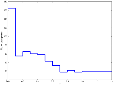
Ideally, the coarse-graining approximation of the $F(z)$ evolution should approach continuity as its limit. However, for our analysis using the data of 557 SNeIa from Union2 and the 13 $H(z)$ measurements, the redshift distribution of data poses a limit on how fine we can dissect the redshift range into bins, hence the resolution of our reconstruction of $F(z)$. Each bin should cover enough data to make the value of $F(z)$ well-constrained inside of it. To this end, we introduce 11 bins equally spaced to cover the redshift range, shown in Figure 1. The first 10 bins are kept to be equal in width, but the last one is widened to cover the diminishing tail of the SNIa redshift distribution.

Figure 1.— Binning of the redshift range to accommodate enough data in each of the bins. The histogram shows the number of SNIa data points distributed across the redshift range, with each bin covering width 0.1.

3.3. Evaluation of the Fisher Matrix

The Fisher matrix elements as defined by equation (11) are statistical averages involving unknown parameters. However, for our purpose we cannot evaluate them by averaging in the absence of a known posterior. In fact, it is neither practical nor logical to do this, as our final models to assess the evaluation of energy conditions are not the model described so far per se, but the models to be built from the principal components extracted from the Fisher matrix.

In practice, the Fisher matrix elements can be estimated at point in the parameter space where the posterior PDF is close to the maximum. In other words, we can approximate the numerical values of the Fisher matrix elements using a fiducial model, which we choose to be the concordance flat $\mathrm{\Lambda CDM}$ model with $\Omega_{\mathrm{m}}=0.274$, $\Omega_{\mathrm{\Lambda}}=0.726$ as favored by combined observational data (Amanullah et al. 2010; Komatsu et al. 2011) and $H_{0}=74.2$ $\mathrm{km\ s^{-1}\ Mpc^{-1}}$ from (Riess et al. 2009). In a similar setting, Shapiro & Turner (2006) used a even simpler, constant-input model as the fiducial one in their analysis, and found the method to be robust against the introducing of a simplified fiducial. Our own findings are in agreement to their claim.

To add robustness and safeguard against limited sampling in the parameter space, we resampling (Efron 1982) to check for any possible bias resulting from not treating the averaging in equation (11) rigorously. The result confirms the robustness of Fisher matrix estimation, and the average from the resampled Fisher matrices are used as the “reference stack” in subsequent steps.

The Fisher matrix elements are thus calculated using the $\tilde{\chi}^{2}$ (or posterior log-PDF) expressions given in the preceding Sections 3.1.1 and 3.1.2. Notice that the normalization constants discarded in the previous steps do not contribute to the matrix elements because they are additive constants in the log-PDF independent of the parameters, and their derivatives vanish.

4. Results

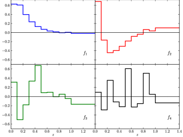
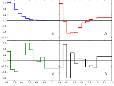
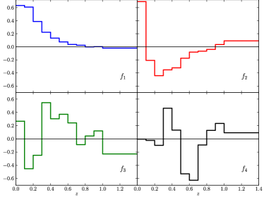
We numerically compute the $(N+1)\times(N+1)$ Fisher matrix for $F(z)$ in each of the $N$ bins and $\Omega_{\mathrm{k}}$. At this stage, the $\Omega_{\mathrm{k}}$ parameter can be effectively marginalized over by projecting the matrix onto the $N\times N$ subspace (Dodelson 2003, Chapter 11). The eigenvectors of the resulting matrix, $f_{i}$, are then retrieved. In this manner, we can thus build a chain of models with successively more parameters. The eigenvectors are the principal components we are after, and they are shown in Figures 2, 3, and 4 for three energy conditions. Then the reconstruction we need can be expressed as a linear combination of the principal components

$$F(z)=\sum_{i}a_{i}f_{i}(z).$$ (23)

Notably, the first three principal components appears stable regardless of which energy condition the reconstruction is for. However, the higher-order and noisier modes show greater change in the form with respected to the energy condition being reconstructed. Furthermore, when reconstructing $F(z)$ by fitting the linear expression (Eq. [23]), the curvature parameter $\Omega_{\mathrm{k}}$ appearing in equations (5) and (6) has been marginalized with numerical integration.

Figure 2.— Four well-constrained principal components of $F_{\mathrm{NEC}}(z)$. They are normalized so that $\int{f^{2}_{i}(z)\mathrm{d}z=1}$. $f_{i}$’s $(i=1,2,3,4)$ are the first four eigenvectors of the Fisher matrix.

Figure 3.— Same as Figure 2 but for $F_{\mathrm{DEC}}(z)$.

Figure 4.— Same as Figure 2 but for $F_{\mathrm{SEC}}(z)$.

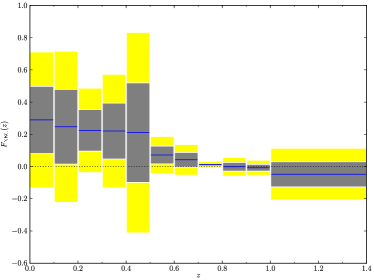
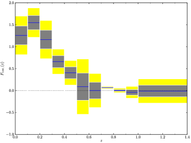
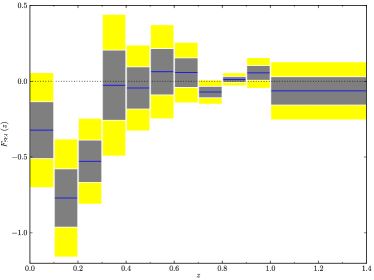
The reconstructed $F(z)$ for the three energy conditions are shown in Figures 5, 6, and 7. We have use only the first three principal components in the fitting of $F(z)$. The fitted values of the coefficients are listed in Table 1.

Table 1Best-fit coefficients of the first three principal components

$a_{i}$	NEC	DEC	SEC
$a_{1}$	$-0.51\pm 0.08$	$\phantom{string}2.40\pm 0.10$	$\phantom{string}0.88\pm 0.08$
$a_{2}$	$\phantom{string}0.12\pm 0.21$	$-0.31\pm 0.22$	$-0.18\pm 0.21$
$a_{3}$	$-0.16\pm 0.45$	$-0.25\pm 0.50$	$-0.43\pm 0.40$

This cutoff from the full spectrum of principal components introduces a well-known artifact, namely a bias at the higher end of the redshift (Shapiro & Turner 2006) that suppresses the reconstructed value and its error bars towards zero. Nevertheless, we note that a value of $F(z)$ close to zero is consistent with our lack of knowledge about the violation of energy conditions by the very construction of $F(z)$. In other words, a vanishing value of $F(z)$ tells us that our bet of finding energy condition fulfillment is no significantly higher or lower than that of finding its violation. Therefore, this bias in the value of $F(z)$ does not tempt us with false claims about energy condition violations, but merely restates our ignorance about it at redshift ranges where there are insufficient data.

Figure 5.— Reconstruction of $F_{\mathrm{NEC}}(z)$ using the first three eigenvectors. The central blue solid line in each bin is the best three-mode fitting result. The gray and yellow bands show 1- and 2-$\sigma$ uncertainties.

Figure 6.— Same as Figure 5 but for $F_{\mathrm{DEC}}(z)$.

Figure 7.— Same as Figure 5 but for $F_{\mathrm{SEC}}(z)$.

5. Conclusion and Discussions

We have explored the likelihood of energy condition violation during the evolution of the universe using the indication functions we proposed in Section 2.1. The indication functions are reconstructed from SNIa and $H(z)$ data.

Our result for NEC does not prefer a history of violation, as is evident from Figure 5. A slight but rising trend can be seen from $z\approx 0.7$ up to now. This trend is more pronounced in our result for DEC presented in Figure 6, and we can be fairly certain that there has been no DEC violation for $z\leq 0.5$.

However, the result for SEC shows fairly strong indication of violation. This shows the view of an accelerating cosmic expansion is compatible with our combination of data, especially for low-redshift ($z\leq 0.3$). Although we have noted the diminishing ability to distinguish energy condition fulfillment from violation at the high-$z$ end, we nevertheless find that our result for SEC hints at a recent transition from deceleration ($F_{\mathrm{SEC}}(z)=q(z)>0$) to acceleration ($F_{\mathrm{SEC}}(z)=q(z)<0$) with the transition redshift $z\approx 0.5$, if we ignore the probably biased result at the high redshift end. This estimation of transition redshift is consistent with the transition redshifts reported by Riess et al. (2004) and Shapiro & Turner (2006) using a kinematic model with $q(z)$ linear in $z$.

For all energy conditions considered, our results show qualitative agreement with previous studies (Visser 1997a, b; Visser & Barceló 2000; Schuecker et al. 2003; Cattoën & Visser 2008). In particular, the clear trend of DEC fulfillment at low redshift is similar to what was found by Lima et al. (2008a, b).

These results are obtained without reference to any specific form of dark energy. With this in mind, we can use these results to assess the feasibility of theoretical dark energy models.

Some models predict that the dark energy component undergoes a transition into the “phantom” phase with the equation of state parameter $w<-1$ (Štefančić 2005, and references therein). It has been noted that NEC (hence necessarily DEC) violation is a feature of these models, and some oscillating universe models predict episodes of NEC violation throughout the history (Cai et al. 2010). Even if certain phenomenological models could offer a fairly good fit (Xia et al. 2005), our data-driven result for NEC suggests that there is not enough motivation to consider them as a viable explanation for cosmic acceleration, at least not in the redshift range investigated in this paper.

On the other hand, a family of dark energy models exist that do not violate NEC or DEC, yet display transient periods of SEC violation (Barrow et al. 2000; Blais & Polarski 2004; Barenboim et al. 2006). While such scenarios are unlikely to have been realized from the early universe up to $z\gtrsim 1$ (Linder 2010; Linder & Smith 2011), from an energy-condition point of view they are not ruled out by our independent results in low redshift. Whether the “returning” $F_{\mathrm{SEC}}$ curve in Figure 7 within $z<0.4$ suggests a coming back to SEC fulfillment, which has been independently noted earlier (Shafieloo et al. 2009; Guimarães & Lima 2011) for spatially flat models, may be worth examining using future data.

As we have already noted in Section 4, our test is sensitive in low redshift but not in high redshift. In the future, this could be partially alleviated by the availability of high-quality cosmological data that could populate higher redshift.

Nevertheless, our work addresses several deficiencies in previous literature and has some special merits.

First, by proposing a set of new models based on our indication functions, we are able to visualize the evolution of the Universe as a history of energy condition violation or fulfillment in a straightforward manner. By construction, we can avoid ambiguous statements such as “SEC implies $H_{0}(z_{f}\approx 15)\leq 58\pm 7$ $\mathrm{km\ s^{-1}\ Mpc^{-1}}$” (paraphrasing Eq. [79] of Visser 1997b), where the inequality nature of the energy conditions find some difficulty being used with error bounds from observational data. Compared with the research done by Lima et al. (2008a), our models and their presentations can be more readily interpreted as answers of “whether an energy condition was violated for a given epoch”, because our indication functions stay constant in each redshift bin.

Second, our models are general and are free from overly restrictive presumptions on the nature of the dark energy. It stands in contrast to previous studies by Schuecker et al. (2003) where a constant equation of state parameter model was used to study the possibility of energy condition violation.

Third, by incorporating the Fisher matrix formalism in our analysis, we find an optimal set of bases for the analysis of energy condition violation in the sense that the coefficients for different modes are nearly uncorrelated. When we generate this set of bases, the effects of $\Omega_{\mathrm{k}}$ are naturally and explicitly taken into account. Compared with the parametrization of Shapiro & Turner (2006), our method is more generally applicable because we do not presume spatial flatness, and has a unified description for all the energy conditions considered. We apply this formalism to the combination of SNIa and $H(z)$ data, and this can be extended to other suitable cosmological probes when the data become available.

References

- Amanullah et al. (2010) Amanullah, R. et al. 2010, ApJ, 716, 712, arXiv:1004.1711
- Barenboim et al. (2006) Barenboim, G., Mena Requejo, O., & Quigg, C. 2006, J. Cosmol. Astropart. Phys., 4, 8, arXiv:astro-ph/0510178
- Barrow et al. (2000) Barrow, J. D., Bean, R., & Magueijo, J. 2000, MNRAS, 316, L41, arXiv:astro-ph/0004321
- Blais & Polarski (2004) Blais, D., & Polarski, D. 2004, Phys. Rev. D, 70, 084008, arXiv:astro-ph/0404043
- Buniy et al. (2006) Buniy, R. V., Hsu, S. D. H., & Murray, B. M. 2006, Phys. Rev. D, 74, 063518, arXiv:hep-th/0606091
- Cai et al. (2010) Cai, Y.-F., Saridakis, E. N., Setare, M. R., & Xia, J.-Q. 2010, Phys. Rep., 493, 1, arXiv:0909.2776
- Caldwell et al. (2003) Caldwell, R. R., Kamionkowski, M., & Weinberg, N. N. 2003, Phys. Rev. Lett., 91, 071301, arXiv:astro-ph/0302506
- Carroll (2004) Carroll, S. M. 2004, Spacetime and Geometry: An Introduction to General Relativity (San Francisco, CA: Addison Wesley)
- Carroll et al. (2003) Carroll, S. M., Hoffman, M., & Trodden, M. 2003, Phys. Rev. D, 68, 023509, arXiv:astro-ph/0301273
- Cattoën & Visser (2008) Cattoën, C., & Visser, M. 2008, Class. Quantum Gravity, 25, 165013, arXiv:0712.1619
- Crittenden et al. (2009) Crittenden, R. G., Pogosian, L., & Zhao, G.-B. 2009, J. Cosmol. Astropart. Phys., 12, 25, arXiv:astro-ph/0510293
- di Pietro & Claeskens (2003) di Pietro, E., & Claeskens, J.-F. 2003, MNRAS, 341, 1299, arXiv:astro-ph/0207332
- Dodelson (2003) Dodelson, S. 2003, Modern Cosmology (San Diego, CA: Academic Press)
- Dubovsky et al. (2006) Dubovsky, S., Grégoire, T., Nicolis, A., & Rattazzi, R. 2006, J. High Energy Phys., 3, 25, arXiv:hep-th/0512260
- Efron (1982) Efron, B. 1982, The Jackknife, the Bootstrap and Other Resampling Plans (Philadelphia, PA: Society for Industrial and Applied Mathematics)
- Gaztañaga et al. (2009) Gaztañaga, E., Cabré, A., & Hui, L. 2009, MNRAS, 399, 1663, arXiv:0807.3551
- Guimarães & Lima (2011) Guimarães, A. C. C., & Lima, J. A. S. 2011, Class. Quantum Gravity, 28, 125026, arXiv:1005.2986
- Hawking & Ellis (1973) Hawking, S. W., & Ellis, G. F. R. 1973, The Large Scale Structure of Space-Time. (Cambridge, United Kingdom: Cambridge University Press)
- Huterer & Cooray (2005) Huterer, D., & Cooray, A. 2005, Phys. Rev. D, 71, 023506, arXiv:astro-ph/0404062
- Huterer & Starkman (2003) Huterer, D., & Starkman, G. 2003, Phys. Rev. Lett., 90, 031301, arXiv:astro-ph/0207517
- Komatsu et al. (2011) Komatsu, E. et al. 2011, ApJS, 192, 18, arXiv:1001.4538
- Krauss & Chaboyer (2003) Krauss, L. M., & Chaboyer, B. 2003, Science, 299, 65
- Lake (2004) Lake, K. 2004, Class. Quantum Gravity, 21, L129, arXiv:gr-qc/0407107
- Li et al. (2011) Li, M., Li, X.-D., Wang, S., & Wang, Y. 2011, Commun. Theor. Phys., 56, 525, arXiv:1103.5870
- Lima et al. (2008a) Lima, M. P., Vitenti, S., & Rebouças, M. J. 2008a, Phys. Rev. D, 77, 083518, arXiv:0802.0706
- Lima et al. (2008b) ——. 2008b, Phys. Lett. B, 668, 83, arXiv:0808.2467
- Linder (2010) Linder, E. V. 2010, Phys. Rev. D, 82, 063514, arXiv:1006.4632
- Linder & Smith (2011) Linder, E. V., & Smith, T. L. 2011, J. Cosmol. Astropart. Phys., 4, 1, arXiv:1009.3500
- Ma & Zhang (2011) Ma, C., & Zhang, T.-J. 2011, ApJ, 730, 74, arXiv:1007.3787
- Nesseris & Perivolaropoulos (2004) Nesseris, S., & Perivolaropoulos, L. 2004, Phys. Rev. D, 70, 043531, arXiv:astro-ph/0401556
- Riess et al. (2004) Riess, A. G., et al. 2004, ApJ, 607, 665, arXiv:astro-ph/0402512
- Riess et al. (2009) ——. 2009, ApJ, 699, 539, arXiv:0905.0695
- Schuecker et al. (2003) Schuecker, P., Caldwell, R. R., Böhringer, H., Collins, C. A., Guzzo, L., & Weinberg, N. N. 2003, A&A, 402, 53, arXiv:astro-ph/0211480
- Shafieloo et al. (2009) Shafieloo, A., Sahni, V., & Starobinsky, A. A. 2009, Phys. Rev. D, 80, 101301, arXiv:0903.5141
- Shapiro & Turner (2006) Shapiro, C., & Turner, M. S. 2006, ApJ, 649, 563, arXiv:astro-ph/0512586
- Simon et al. (2005) Simon, J., Verde, L., & Jimenez, R. 2005, Phys. Rev. D, 71, 123001, arXiv:astro-ph/0412269
- Stern et al. (2010) Stern, D., Jimenez, R., Verde, L., Kamionkowski, M., & Stanford, S. A. 2010, J. Cosmol. Astropart. Phys., 2, 8, arXiv:0907.3149
- Štefančić (2005) Štefančić, H. 2005, Phys. Rev. D, 71, 124036, arXiv:astro-ph/0504518
- Visser (1997a) Visser, M. 1997a, Science, 276, 88, arXiv:gr-qc/9710010
- Visser (1997b) ——. 1997b, Phys. Rev. D, 56, 7578, arXiv:gr-qc/9705070
- Visser & Barceló (2000) Visser, M., & Barceló, C. 2000, in COSMO-99: International Workshop on Particle Physics and the Early Universe, ed. U. Cotti, R. Jeannerot, G. Senjanovi, & A. Smirnov, 98–112, arXiv:gr-qc/0001099
- Wald (1984) Wald, R. M. 1984, General Relativity (Chicago, IL: University of Chicago Press)
- Xia et al. (2005) Xia, J.-Q., Feng, B., & Zhang, X. 2005, Mod. Phys. Lett. A, 20, 2409, arXiv:astro-ph/0411501
- Zhang & Zhu (2008) Zhang, H., & Zhu, Z.-H. 2008, J. Cosmol. Astropart. Phys., 3, 7, arXiv:astro-ph/0703245
- Zhang et al. (2010) Zhang, T.-J., Ma, C., & Lan, T. 2010, Adv. Astron., 2010, arXiv:1010.1307
- Zhao & Zhang (2010) Zhao, G.-B., & Zhang, X. 2010, Phys. Rev. D, 81, 043518, arXiv:0908.1568