Learning Hierarchical and Topographic Dictionaries
with Structured Sparsity

Abstract

Recent work in signal processing and statistics have focused on defining new regularization functions, which not only induce sparsity of the solution, but also take into account the structure of the problem [(1), (2), (3), (4), (5), (6), (7)]. We present in this paper a class of convex penalties introduced in the machine learning community, which take the form of a sum of $\ell_{2}$- and $\ell_{\infty}$-norms over groups of variables. They extend the classical group-sparsity regularization[(8), (9), (10)] in the sense that the groups possibly overlap, allowing more flexibility in the group design. We review efficient optimization methods to deal with the corresponding inverse problems [(11), (12), (13)], and their application to the problem of learning dictionaries of natural image patches [(14), (15), (16), (17), (18)]: On the one hand, dictionary learning has indeed proven effective for various signal processing tasks [(17), (19)]. On the other hand, structured sparsity provides a natural framework for modeling dependencies between dictionary elements. We thus consider a structured sparse regularization to learn dictionaries embedded in a particular structure, for instance a tree [(11)] or a two-dimensional grid [(20)]. In the latter case, the results we obtain are similar to the dictionaries produced by topographic independent component analysis [(21)].

1 INTRODUCTION

Sparse representations have recently drawn much interest in signal, image, and video processing. Under the assumption that natural images admit a sparse decomposition in some redundant basis (or so-called dictionary), several such models have been proposed, e.g., curvelets[(22)], wedgelets[(23)], bandlets [(24)] and more generally various sorts of wavelets[(25)]. Learned sparse image models were first introduced in the neuroscience community by Olshausen and Field[(14), (15)] for modeling the spatial receptive fields of simple cells in the mammalian visual cortex. The linear decomposition of a signal using a few atoms of a learned dictionary instead of predefined ones, has recently led to state-of-the-art results for numerous low-level image processing tasks such as denoising, inpainting [(17), (19), (26)] or texture synthesis [(27)], showing that sparse models are well adapted to natural images. Unlike decompositions based on principal component analysis, these models can rely on overcomplete dictionaries, with a number of atoms greater than the original dimension of the signals, allowing more flexibility to adapt the representation to the data.

In addition to this recent interest from the signal and image processing communities for sparse modelling, statisticians have developed similar tools from a different point of view. In signal processing, one often represents a data vector ${\mathbf{y}}$ of fixed dimension $m$ as a linear combination of $p$ dictionary elements ${\mathbf{D}}=[{\mathbf{d}}^{1},\ldots,{\mathbf{d}}^{p}]$ in ${\mathbb{R}}^{m\times p}$. In other words, one looks for a vector ${\boldsymbol{\alpha}}$ in ${\mathbb{R}}^{p}$ such that ${\mathbf{y}}\approx{\mathbf{D}}{\boldsymbol{\alpha}}$. When we assume ${\boldsymbol{\alpha}}$ to be sparse—that is has a lot of zero coefficients, we obtain a sparse linear model and need appropriate regularization functions. When ${\mathbf{D}}$ is fixed, the columns ${\mathbf{d}}^{i}$ can be interpreted as the elements of a redundant basis, for instance wavelets [(25)].

Let us now consider a different problem occurring in statistics or machine learning. Given a training set $(y^{i},{\mathbf{x}}^{i})_{i=1}^{m}$, where the $y^{i}$’s are scalars, and the ${\mathbf{x}}^{i}$’s are vectors in ${\mathbb{R}}^{p}$, the task is to predict a value for $y$ from an observation ${\mathbf{x}}$ in ${\mathbb{R}}^{p}$. This is usually achieved by learning a model from the training data, and the simplest one is to assume that there exists a linear relationship $y\approx{\mathbf{x}}^{\top}{\mathbf{w}}$, where ${\mathbf{w}}$ is a vector in ${\mathbb{R}}^{p}$. Learning the model amounts to adapt ${\mathbf{w}}$ to the training set and denoting by ${\mathbf{y}}$ the vector in ${\mathbb{R}}^{n}$ whose entries are the $y^{i}$’s, and ${\mathbf{X}}$ the matrix in ${\mathbb{R}}^{m\times p}$ the matrix whose rows are the ${\mathbf{x}}^{i}$’s, we end up looking for a vector ${\mathbf{w}}$ such that ${\mathbf{y}}\approx{\mathbf{X}}{\mathbf{w}}$. When one knows in advance that the vector ${\mathbf{w}}$ is sparse, a similar problem as in signal processing is raised, where ${\mathbf{X}}$ can be interpreted as a “dictionary” but is often called a set of “features” or “predictors”. This is therefore not surprising that both communities have developed similar tools, the Lasso formulation [(28)], L2-boosting algorithm[(29)], forward selection techniques[(30)] in statistics are respectively equivalent (up to minor details) to the basis pursuit problem [(31)], matching and variants of orthogonal matching pursuit algorithms[(32)].

Formally, the sparse decomposition problem of a signal ${\mathbf{y}}$ using a dictionary ${\mathbf{D}}$ amounts to finding a vector ${\boldsymbol{\alpha}}$ minimizing the following cost function

$$\min_{{\boldsymbol{\alpha}}\in{\mathbb{R}}^{p}}\frac{1}{2}\|{\mathbf{y}}-{\mathbf{D}}{\boldsymbol{\alpha}}\|_{2}^{2}+\lambda\psi({\boldsymbol{\alpha}}),$$ (1)

where $\psi$ is a sparsity-inducing function, and $\lambda$ a regularization parameter. A natural choice is to use the $\ell_{0}$ quasi-norm, which counts the number of non-zero elements in a vector, leading however to an NP-hard problem[(33)], which is usually tackled with greedy algorithms [(32)]. Another approach consists of using a convex relaxation such as the $\ell_{1}$-norm. Indeed, it is well known that the $\ell_{1}$ penalty yields a sparse solution, but there is no analytic link between the value of $\lambda$ and the effective sparsity $\|{\mathbf{x}}\|_{0}$ that it yields.

We consider in this paper recent sparsity-inducing penalties capable of encoding the structure of a signal decomposition on a redundant basis. The $\ell_{1}$-norm primarily encourages sparse solutions, regardless of the potential structural relationships (e.g., spatial, temporal or hierarchical) existing between the variables. To cope with that issue, some effort has recently been devoted to designing sparsity-inducing regularizations capable of encoding higher-order information about the patterns of non-zero coefficients, some of these works coming from the machine learning/statistics literature [(2), (3), (1), (4)] others from signal processing [(5)]. We use here the approach of Jenatton et al. [(2)] who consider sums of norms of appropriate subsets, or groups, of variables, in order to control the sparsity patterns of the solutions. The underlying optimization is usually difficult, in part because it involves nonsmooth components. We review strategies to address these problems, first when the groups are embedded in a tree [(1), (11)], second in a general setting [(13)].

Whereas these penalties have been shown to be useful for solving various problems in computer vision, bio-informatics, or neuroscience [(2), (3), (1), (4)], we address here the problem of learning dictionaries of natural image patches which exhibit particular relationships among their elements. Such a construction is motivated a priori by two distinct but related goals: first to potentially improve the performance of denoising, inpainting or other signal processing tasks that can be tackled based on the learned dictionaries, and second to uncover or reveal some of the natural structures present in images. In previous work[(11)], we have for instance embedded dictionary elements into a tree, by using a hierarchical norm [(1)]. This model encodes a rule saying that a dictionary element can be used in the decomposition of a signal only if its ancestors in the tree are used as well, similarly as in the zerotree wavelet model [(34)]. In the related context of independent component analysis (ICA), Hyvärinen et al.[(21)] have arranged independent components (corresponding to dictionary elements) on a two-dimensional grid, and have modelled spatial dependencies between them. When learned on whitened natural image patches, this model exhibits “Gabor-like” functions which are smoothly organized on the grid, which the authors call a topographic map. As shown in Ref. kavukcuoglu2 [20], such a result can be reproduced with a dictionary learning formulation using structured regularization.

We use the following notation in the paper: Vectors are denoted by bold lower case letters and matrices by upper case ones. We define for $q\geq 1$ the $\ell_{q}$-norm of a vector ${\mathbf{x}}$ in ${\mathbb{R}}^{m}$ as $\|{\mathbf{x}}\|_{q}\triangleq(\sum_{i=1}^{m}|{\mathbf{x}}_{i}|^{q})^{{1}/{q}}$, where ${\mathbf{x}}_{i}$ denotes the $i$-th coordinate of ${\mathbf{x}}$, and $\|{\mathbf{x}}\|_{\infty}\triangleq\max_{i=1,\ldots,m}|{\mathbf{x}}_{i}|=\lim_{q\to\infty}\|{\mathbf{x}}\|_{q}$. We also define the $\ell_{0}$-pseudo-norm as the number of nonzero elements in a vector: $\|{\mathbf{x}}\|_{0}\triangleq\#\{i~{}~{}\text{s.t.}~{}~{}{\mathbf{x}}_{i}\neq 0\}=\lim_{q\to 0^{+}}(\sum_{i=1}^{m}|{\mathbf{x}}_{i}|^{q})$. We consider the Frobenius norm of a matrix ${\mathbf{X}}$ in ${\mathbb{R}}^{m\times n}$: $\left\|{\mathbf{X}}\right\|_{\text{F}}\triangleq(\sum_{i=1}^{m}\sum_{j=1}^{n}{\mathbf{X}}_{ij}^{2})^{{1}/{2}}$, where ${\mathbf{X}}_{ij}$ denotes the entry of ${\mathbf{X}}$ at row $i$ and column $j$.

This paper is structured as follows: Section 2 reviews the dictionary learning and structured sparsity frameworks, Section 3 is devoted to optimization techniques, and Section 4 to experiments with structured dictionary learning. Note that the material of this paper relies upon two of our papers published in the Journal of Machine Learning Research [(13), (11)].

2 RELATED WORK

We present in this section the dictionary learning framework and structured sparsity-inducing regularization functions.

2.1 Dictionary Learning

Consider a signal ${\mathbf{y}}$ in ${\mathbb{R}}^{m}$. We say that ${\mathbf{y}}$ admits a sparse approximation over a dictionary ${\mathbf{D}}$ in ${\mathbb{R}}^{m\times p}$, composed of $p$ elements (atoms), when we can find a linear combination of a “few” atoms from ${\mathbf{D}}$ that is “close” to the original signal ${\mathbf{x}}$. A number of practical algorithms have been developed for learning such dictionaries like the K-SVD algorithm [(35)], the method of optimal directions (MOD) [(16)], stochastic gradient descent algorithms [(14)] or other online learning techniques [(18)], which will be briefly reviewed in Section 3. This approach has led to several restoration algorithms, with state of the art results in image and video denoising, inpainting, demosaicing [(17), (19)], and texture synthesis [(27)].

Given a training set of signals ${\mathbf{Y}}=[{\mathbf{y}}^{1},\ldots,{\mathbf{y}}^{n}]$ in ${\mathbb{R}}^{m\times n}$, such as natural image patches, dictionary learning amounts to finding a dictionary which is adapted to every signal ${\mathbf{y}}^{i}$, in other words it can be cast as the following optimization problem

$$\min_{{\mathbf{D}}\in{\mathcal{C}},{\mathbf{A}}\in{\mathbb{R}}^{p\times n}}\sum_{i=1}^{n}\frac{1}{2}\|{\mathbf{y}}^{i}-{\mathbf{D}}{\boldsymbol{\alpha}}^{i}\|_{2}^{2}+\lambda\psi({\boldsymbol{\alpha}}^{i}),$$ (2)

where ${\mathbf{A}}=[{\boldsymbol{\alpha}}^{1},\ldots,{\boldsymbol{\alpha}}^{n}]$ are decomposition coefficients, $\psi$ is a sparsity-inducing penalty, and ${\mathcal{C}}$ is a constraint set, typically the set of matrices whose columns have less than unit $\ell_{2}$-norm:

$${\mathcal{C}}\triangleq\{{\mathbf{D}}\in{\mathbb{R}}^{m\times p}:\forall j=1,\ldots,p,~{}~{}~{}~{}\|{\mathbf{d}}^{j}\|_{2}\leq 1\}.$$ (3)

To prevent ${\mathbf{D}}$ from being arbitrarily large (which would lead to arbitrarily small values of ${\boldsymbol{\alpha}}$), it is indeed necessary to constrain the dictionary with such a set ${\mathcal{C}}$. We also remark that dictionary learning is an instance of matrix factorization problem, which can be equivalently rewritten

$$\min_{{\mathbf{D}}\in{\mathcal{C}},{\mathbf{A}}\in{\mathbb{R}}^{p\times n}}\frac{1}{2}\|{\mathbf{Y}}-{\mathbf{D}}{\mathbf{A}}\|_{\text{F}}^{2}+\lambda\psi^{\prime}({\mathbf{A}}),$$ (4)

with an appropriate function $\psi^{\prime}$. Noticing this interpretation of dictionary learning as a matrix factorization has a number of practical consequences. With adequate constraints on ${\mathbf{A}}$ and ${\mathbf{D}}$, one can indeed recast several classical problems as regularized matrix factorization problems, for instance principal component analysis (PCA), non-negative matrix factorization (NMF)[(36)], hard and soft vector quantization (VQ). As a first consequence, all of these approaches can be addressed with similar algorithms, as shown in Ref. mairal7 [18]. A natural approach to approximately solve this non-convex problem is for instance to alternate between the optimization of ${\mathbf{D}}$ and ${\mathbf{A}}$ in Eq. (4), minimizing over one while keeping the other one fixed[(16)], a technique also used in the K-means algorithm for vector quantization.

Another approach consists of using stochastic approximations and use online learning algorithms. When $n$ is large, finding the sparse coefficients ${\mathbf{A}}$ with a fixed dictionary ${\mathbf{D}}$ requires solving $n$ sparse decomposition problems (1), which can be cumbersome. To cope with this issue, online learning techniques adopt a different iterative algorithmic scheme: At iteration $t$, they randomly draw one signal ${\mathbf{y}}^{t}$ from the training set (or a mini-batch), and try to “improve” ${\mathbf{D}}$ given this observation. Assume indeed that $n$ is large and that the image patches ${\mathbf{y}}^{i}$ are i.i.d. samples drawn from an unknown distribution $p({\mathbf{y}})$, then Eq. (2) is asymptotically equivalent to

$$\min_{{\mathbf{D}}\in{\mathcal{C}}}{\mathbb{E}}_{{\mathbf{y}}\sim p({\mathbf{y}})}\left[\min_{{\boldsymbol{\alpha}}\in{\mathbb{R}}^{p}}\frac{1}{2}\|{\mathbf{y}}-{\mathbf{D}}{\boldsymbol{\alpha}}\|_{2}^{2}+\lambda\psi({\boldsymbol{\alpha}})\right].$$ (5)

In order to optimize a cost function which includes an expectation, it is natural to use stochastic approximations[(37)]. When $\psi$ is the $\ell_{1}$-norm, this problem is also under mild assumptions differentiable (see Mairal et al.[(18)] for more details), and a first order stochastic gradient descent step[(15), (18)], given a signal ${\mathbf{y}}^{t}$ can can be written:

$${\mathbf{D}}\leftarrow\Pi_{\mathcal{C}}\Big{[}{\mathbf{D}}+\delta_{t}({\mathbf{y}}^{t}-{\mathbf{D}}{\boldsymbol{\alpha}}^{t}){\boldsymbol{\alpha}}^{t\top})\Big{]},$$ (6)

where $\delta_{t}$ is the gradient step, $\Pi_{\mathcal{C}}$ is the orthogonal projector onto ${\mathcal{C}}$. The vector ${\boldsymbol{\alpha}}^{t}$ carries the sparse coefficients obtained from the decomposition of ${\mathbf{y}}^{t}$ with the current dictionary ${\mathbf{D}}$. When $\psi$ is the $\ell_{0}$-norm, this iteration is heuristic but gives good results in practice, when $\psi$ is the $\ell_{1}$-norm, and assuming the solution of the sparse decomposition problem to be unique, this iteration exactly corresponds to a stochastic gradient descent algorithm[(37)]. Note that the vectors ${\mathbf{y}}^{t}$ are assumed to be i.i.d. samples of the (unknown) distribution $p({\mathbf{y}})$. Even though it is often difficult to obtain such i.i.d. samples, the vectors ${\mathbf{y}}^{t}$ are in practice obtained by cycling on a randomly permuted training set. The main difficulty in this approach is to take a good learning rate $\delta_{t}$. Other dedicated online learning algorithms have been proposed [(18)], which can be shown to provide a stationary point of the optimization problem (5). All of these online learning techniques have shown to yield significantly speed-ups over classical alternative minimization approach, when $n$ is large enough.

Examples of dictionaries learned using the approach of Mairal et al.[(18)] are represented in Figure 1, and exhibit intriguing visual results. Some of the dictionary elements look like Gabor wavelets, whereas other elements are more difficult to interpret. As for the color image patches, we observe that most of the dictionary elements are gray, with a few low-frequency colored elements exhibiting complementary colors, a phenomenon already observed in image processing applications [(19)].

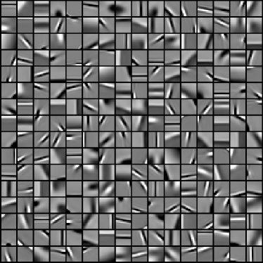
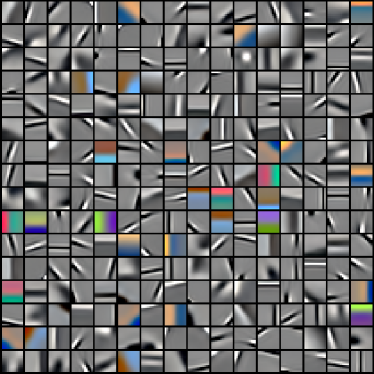
Figure 1: Examples of dictionary with $p=256$ elements, learned on a database of $10$ million natural $12\times 12$ image patches when $\psi$ is the $\ell_{1}$-norm, for grayscale patches on the left, and color patches in the right (after removing the mean color of each patch). Image taken from Ref. mairal_thesis [38].

2.2 Structured Sparsity

We consider again the sparse decomposition problem presented in Eq. (1), but we allow $\psi$ to be different than the $\ell_{0}$ or $\ell_{1}$-regularization, and we are interested in problems where the solution is beforehand not only assumed to be sparse —that is, the solution has only a few non-zero coefficients, but also to form non-zero patterns with a specific structure. It is indeed possible to encode additional knowledge in the regularization other than just sparsity. For instance, one may want the non-zero patterns to be structured in the form of non-overlapping groups [(8), (9), (10)], in a tree [(1), (11)], or in overlapping groups [(2), (3), (4), (5), (6), (7)]. As for classical non-structured sparse models, there are basically two lines of research, that either (a) deal with nonconvex and combinatorial formulations that are in general computationally intractable and addressed with greedy algorithms or (b) concentrate on convex relaxations solved with convex programming methods. We focus in this paper on the latter.

When the sparse coefficients are organized in groups, a penalty encoding explicitly this prior knowledge can improve the prediction performance and/or interpretability of the learned models [(9), (10)]. Denoting by ${\mathcal{G}}$ a set of groups of indices, such a penalty takes the form:

$$\psi({\boldsymbol{\alpha}})\,\triangleq\,\sum_{g\in{\mathcal{G}}}\eta_{g}\|{\boldsymbol{\alpha}}_{g}\|_{q},$$ (7)

where ${\boldsymbol{\alpha}}_{j}$ is the $j$-th entry of ${\boldsymbol{\alpha}}$ for $j$ in $[1;p]\triangleq\{1,\ldots,p\}$, the vector ${\boldsymbol{\alpha}}_{g}$ in $\mathbb{R}^{|g|}$ records the coefficients of ${\boldsymbol{\alpha}}$ indexed by $g$ in ${\mathcal{G}}$, and the scalars $\eta_{g}$ are positive weights. $\|.\|_{q}$ denotes here either the $\ell_{2}$ or $\ell_{\infty}$-norms. Note that when ${\mathcal{G}}$ is the set of singletons of $[1;p]$, we get back the $\ell_{1}$-norm. Inside a group, the $\ell_{2}$- or $\ell_{\infty}$-norm does not induce sparsity, whereas the sum over the groups can be interpreted as an $\ell_{1}$-norm and indeed, when ${\mathcal{G}}$ is a partition of $[1;p]$, variables are selected in groups rather than individually. When the groups overlap, $\psi$ is still a norm and sets groups of variables to zero together [(2)]. The latter setting has first been considered for hierarchies [(1)], and then extended to general group structures [(2)]. Solving Eq. (1) in this context becomes challenging and is the topic of the next section. Before that, in order to better illustrate how such norms should be used and how to design a group structure inducing a desired sparsifying effect, we proceed by giving a few examples of group structures.

2.2.1 One-dimensional Sequence.

Given $p$ variables organized in a sequence, suppose we want to select only contiguous nonzero patterns. A set of groups $\mathcal{G}$ exactly producing such patterns is represent on Figure 2. It is indeed easy to show that by selecting a family of groups in $\mathcal{G}$ represented in this figure, and setting the corresponding variables to zero, exactly leads to contiguous patterns of non-zero coefficients. The penalty (7) with this group structure produces therefore exactly the desired sparsity patterns.

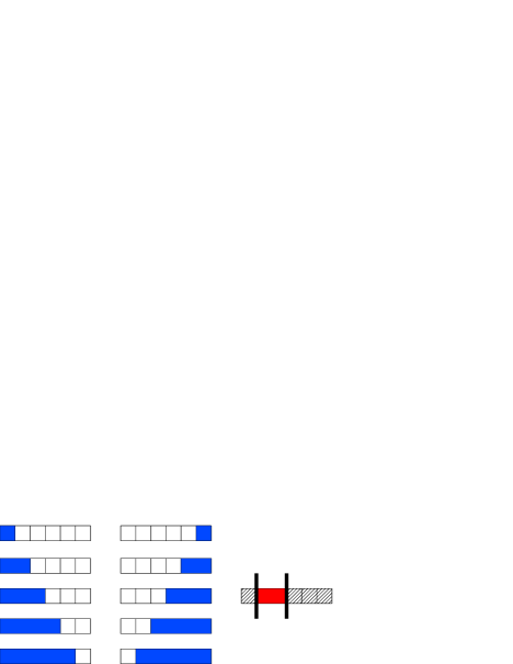
Figure 2: (Left) The set of blue groups to penalize in order to select contiguous patterns in a sequence. (Right) In red, an example of such a nonzero pattern with its corresponding zero pattern (hatched area). Image taken from Ref. jenatton [2].

2.2.2 Hierarchical Norms

Another example of interest originally comes from the wavelet literature. It consists of modelling hierarchical relations between wavelet coefficients, which are naturally organized in a tree, due to the multiscale properties of wavelet decompositions.[(25)] The zero-tree wavelet model[(34)] indeed assumes that if a wavelet coefficient is set to zero, then it should be the case for all its descendants in the tree. This effect can in fact be exactly achieved with the convex regularization of Eq. (7), with an appropriate group structure presented in Figure 3. This penalty was originally introduced in the statistics community by Zhao et al.[(1)], and found different applications, notably in topic models for text corpora [(11)].

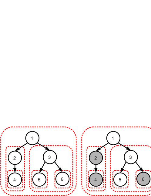
Figure 3: Left: example of a tree-structured set of groups $\mathcal{G}$ (dashed contours in red), corresponding to a tree $\mathcal{T}$ with $p=6$ nodes represented by black circles. Right: example of a sparsity pattern induced by the tree-structured norm corresponding to $\mathcal{G}$: the groups $\{2,4\},\{4\}$ and $\{6\}$ are set to zero, so that the corresponding nodes (in gray) that form subtrees of $\mathcal{T}$ are removed. The remaining nonzero variables $\{1,3,5\}$ form a rooted and connected subtree of $\mathcal{T}$. This sparsity pattern obeys the following equivalent rules: (i) if a node is selected, so are all of its ancestors. (ii) if a node is not selected, then its descendant are not selected. Image taken from Ref. jenatton4 [11].

2.2.3 Neighborhoods on a 2D-Grid

Another group structure we are going to consider corresponds to the assumption that the dictionary elements can be organized on a 2D-grid, for example we might have $p=20\times 20$ dictionary elements. To obtain a spatial regularization effect on the grid, it is possible to use as groups all the $e\times e$ neighborhoods on the grid, for example $3\times 3$. The main effect of such a regularization is to encourage variables that are in a same neighborhood to be set to zero all together. Such dictionary structure has been used for instance in Ref. mairal11 [13] for a background subtraction task (segmenting foreground objects from the background in a video).

3 OPTIMIZATION FOR STRUCTURED SPARSITY

We now present optimization techniques to solve Eq. (1) when $\psi$ is a structured norm (7). This is the main difficulty to overcome to learn structured dictionaries. We review here the techniques introduced in Refs. jenatton4 [11, 13]. More details can be found in these two papers. Other technique for dealing with sparsity-inducing penalties can also be found in Ref. bach5 [39].

3.1 Proximal Gradient Methods

In a nutshell, proximal methods can be seen as a natural extension of gradient-based techniques, and they are well suited to minimizing the sum $f+\lambda\psi$ of two convex terms, a smooth function $f$ —continuously differentiable with Lipschitz-continuous gradient— and a potentially non-smooth function $\lambda\psi$ (see Refs. combette [40, 39] and references therein). In our context, the function $f$ takes the form $f({\boldsymbol{\alpha}})=\frac{1}{2}\|{\mathbf{y}}-{\mathbf{D}}{\boldsymbol{\alpha}}\|_{2}^{2}$. At each iteration, the function $f$ is linearized at the current estimate ${\boldsymbol{\alpha}}_{0}$ and the so-called proximal problem has to be solved:

$$\min_{{\boldsymbol{\alpha}}\in\mathbb{R}^{p}}f({\boldsymbol{\alpha}}_{0})+({\boldsymbol{\alpha}}-{\boldsymbol{\alpha}}_{0})^{\top}\nabla f({\boldsymbol{\alpha}}_{0})+\lambda\psi({\boldsymbol{\alpha}})+{\displaystyle\frac{L}{2}}\|{\boldsymbol{\alpha}}-{\boldsymbol{\alpha}}_{0}\|_{2}^{2}.$$

The quadratic term keeps the solution in a neighborhood where the current linear approximation holds, and $L\!>\!0$ is an upper bound on the Lipschitz constant of $\nabla f$. This problem can be rewritten as

$$\min_{{\boldsymbol{\alpha}}\in\mathbb{R}^{p}}{\displaystyle\frac{1}{2}}\left\|{\boldsymbol{\beta}}-{\boldsymbol{\alpha}}\right\|_{2}^{2}+\lambda^{\prime}\psi({\boldsymbol{\alpha}}),$$ (8)

with $\lambda^{\prime}\triangleq\lambda/L$, and ${\boldsymbol{\beta}}\triangleq{\boldsymbol{\alpha}}_{0}-\frac{1}{L}\nabla f({\boldsymbol{\alpha}}_{0})$. We call proximal operator associated with the regularization $\lambda^{\prime}\psi$ the function that maps a vector ${\boldsymbol{\beta}}$ in $\mathbb{R}^{p}$ onto the (unique, by strong convexity) solution ${\boldsymbol{\alpha}}^{\star}$ of Eq. (8). Simple proximal methods use ${\boldsymbol{\alpha}}^{\star}$ as the next iterate, but accelerated variants [(41), (42)] are also based on the proximal operator and require to solve problem (8) efficiently to enjoy their fast convergence rates.

This has been shown to be possible in many cases:

• When $\psi$ is the $\ell_{1}$-norm—that is $\psi({\boldsymbol{\alpha}})=\|{\boldsymbol{\alpha}}\|_{1}$— the proximal operator is the well-known elementwise soft-thresholding operator,

  $$\forall j\in[1;p],~{}~{}{\boldsymbol{\beta}}_{j}\mapsto\operatorname{sign}({\boldsymbol{\beta}}_{j})(|{\boldsymbol{\beta}}_{j}|-\lambda)_{+}~{}~{}~{}=\begin{cases}0&\text{if}~{}~{}|{\boldsymbol{\beta}}_{j}|\leq\lambda\\ \operatorname{sign}({\boldsymbol{\beta}}_{j})(|{\boldsymbol{\beta}}_{j}|-\lambda)&\text{otherwise}.\end{cases}$$

• When $\psi$ is a group-Lasso penalty with $\ell_{2}$-norms—that is, $\psi({\boldsymbol{\beta}})=\sum_{g\in{\mathcal{G}}}\|{\boldsymbol{\beta}}_{g}\|_{2}$, with ${\mathcal{G}}$ being a partition of $[1;p]$, the proximal problem is separable in every group, and the solution is a generalization of the soft-thresholding operator to groups of variables:

  $$\forall g\in\mathcal{G}~{}~{},{\boldsymbol{\beta}}_{g}\mapsto{\boldsymbol{\beta}}_{g}-\Pi_{\|.\|_{2}\leq\lambda}[{\boldsymbol{\beta}}_{g}]=\begin{cases}0&\text{if}~{}~{}\|{\boldsymbol{\beta}}_{g}\|_{2}\leq\lambda\\ \frac{\|{\boldsymbol{\beta}}_{g}\|_{2}-\lambda}{\|{\boldsymbol{\beta}}_{g}\|_{2}}{\boldsymbol{\beta}}_{g}&\text{otherwise},\\ \end{cases}$$

  where $\Pi_{\|.\|_{2}\leq\lambda}$ denotes the orthogonal projection onto the ball of the $\ell_{2}$-norm of radius $\lambda$.

• When $\psi$ is a group-Lasso penalty with $\ell_{\infty}$-norms—that is, $\psi({\boldsymbol{\beta}})=\sum_{g\in\mathcal{G}}\|{\boldsymbol{\beta}}_{g}\|_{\infty}$, with ${\mathcal{G}}$ being a partition of $[1;p]$, the solution is a different group-thresholding operator:

  $$\forall g\in\mathcal{G},~{}~{}{\boldsymbol{\beta}}_{g}\mapsto{\boldsymbol{\beta}}_{g}-\Pi_{\|.\|_{1}\leq\lambda}[{\boldsymbol{\beta}}_{g}],$$

  where $\Pi_{\|.\|_{1}\leq\lambda}$ denotes the orthogonal projection onto the $\ell_{1}$-ball of radius $\lambda$, which can be solved in $O(p)$ operations [(43), (44)]. Note that when $\|{\boldsymbol{\beta}}_{g}\|_{1}\leq\lambda$, we have a group-thresholding effect, with ${\boldsymbol{\beta}}_{g}-\Pi_{\|.\|_{1}\leq\lambda}[{\boldsymbol{\beta}}_{g}]=0$.

• When $\psi$ is a tree-structured sum of $\ell_{2}$- or $\ell_{\infty}$-norms as introduced by Ref. zhao [1]—meaning that two groups are either disjoint or one is included in the other, the solution admits a closed form. Let $\preceq$ be a total order on $\mathcal{G}$ such that for $g_{1},g_{2}$ in $\mathcal{G}$, $g_{1}\preceq g_{2}$ if and only if either $g_{1}\subset g_{2}$ or $g_{1}\cap g_{2}=\emptyset$. Then, if $g_{1}\preceq\ldots\preceq g_{|\mathcal{G}|}$, and if we define $\text{Prox}^{g}$ as (a) the proximal operator ${\boldsymbol{\beta}}_{g}\mapsto\text{Prox}_{\lambda\eta_{g}\|\cdot\|}({\boldsymbol{\beta}}_{g})$ on the subspace corresponding to group $g$ and (b) the identity on the orthogonal, it is shown in Ref. jenatton4 [11] that:

  $$\text{Prox}_{\lambda\psi}=\text{Prox}^{g_{m}}\circ\ldots\circ\text{Prox}^{g_{1}},$$ (9)

  which can be computed in $O(p)$ operations. It also includes the sparse group Lasso (sum of group-Lasso penalty and $\ell_{1}$-norm) of Refs. friedman2 [45] and sprechmann [46].

• When the groups overlap but do not have a tree structure, computing the proximal operator is more difficult, but it can still be done efficiently when $q=\infty$. Indeed, as shown by Mairal et al. [(12)], there exists a dual relation between such an operator and a quadratic min-cost flow problem on a particular graph, which can be tackled using network flow optimization techniques. Moreover, it may be extended to more general situations where structured sparsity is expressed through submodular functions [(47)].

Mainly using the tools of Refs. jenatton4 [11, 12], we are therefore able to efficiently solve Eq. (1), either in the case of hierarchical norms with $\ell_{2}$- or $\ell_{\infty}$-norms, or with general group structures with $\ell_{\infty}$-norms. This is one of the main requirements to be able to learn structured dictionary. The next section presents a different optimization technique, adapted to any group structure with $\ell_{2}$- or $\ell_{\infty}$-norms.

3.2 Augmenting Lagrangian Techniques

We consider a class of algorithms which leverage the concept of variable splitting [(40), (48), (49), (50)]. The key is to introduce additional variables ${\boldsymbol{\beta}}^{g}$ in ${\mathbb{R}}^{|g|}$, one for every group $g$ in ${\mathcal{G}}$, and equivalently reformulate Eq. (1) as

$$\min_{\begin{subarray}{c}{\boldsymbol{\alpha}}\in{\mathbb{R}}^{p}\\ {\boldsymbol{\beta}}^{g}\in{\mathbb{R}}^{|g|}\ \text{for}\ g\in{\mathcal{G}}\end{subarray}}f({\boldsymbol{\alpha}})+\lambda\sum_{g\in{\mathcal{G}}}\eta_{g}\|{\boldsymbol{\beta}}^{g}\|_{q}~{}~{}\text{s.t.}~{}~{}\forall g\in{\mathcal{G}},~{}~{}{\boldsymbol{\beta}}^{g}={\boldsymbol{\alpha}}_{g},$$ (10)

The issue of overlapping groups is removed, but new constraints and variables are added.

To solve this problem, it is possible to use the so-called alternating direction method of multipliers (ADMM) [(40), (48), (49), (50)]. It introduces dual variables $\nu^{g}$ in ${\mathbb{R}}^{|g|}$ for all $g$ in ${\mathcal{G}}$, and defines the augmented Lagrangian:

$${\mathcal{L}}\big{(}{\boldsymbol{\alpha}},({\boldsymbol{\beta}}^{g})_{g\in\mathcal{G}},(\nu^{g})_{g\in\mathcal{G}}\big{)}\triangleq f({\boldsymbol{\alpha}})+\sum_{g\in{\mathcal{G}}}\big{[}\lambda\eta_{g}\|{\boldsymbol{\beta}}^{g}\|+\nu^{g\top}({\boldsymbol{\beta}}^{g}-{\boldsymbol{\alpha}}_{g})+\frac{\gamma}{2}\|{\boldsymbol{\beta}}^{g}-{\boldsymbol{\alpha}}_{g}\|_{2}^{2}\big{]},$$

where $\gamma>0$ is a parameter. It is easy to show that solving Eq. (10) amounts to finding a saddle-point of the augmented Lagrangian. The ADMM algorithm finds such a saddle-point by iterating between the minimization of ${\mathcal{L}}$ with respect to each primal variable, keeping the other ones fixed, and gradient ascent steps with respect to the dual variables. More precisely, it can be summarized as:

1. Minimize ${\mathcal{L}}$ with respect to ${\boldsymbol{\alpha}}$, keeping the other variables fixed.

2. Minimize ${\mathcal{L}}$ with respect to the ${\boldsymbol{\beta}}^{g}$’s, keeping the other variables fixed. The solution can be obtained in closed form: for all $g$ in $\mathcal{G}$, ${\boldsymbol{\beta}}^{g}\leftarrow\text{prox}_{\frac{\lambda\eta_{g}}{\gamma}\|.\|}[{\boldsymbol{\alpha}}_{g}-\frac{1}{\gamma}\nu^{g}]$.

3. Take a gradient ascent step on ${\mathcal{L}}$ with respect to the $\nu^{g}$’s: $\nu^{g}\leftarrow\nu^{g}+\gamma({\boldsymbol{\beta}}^{g}-{\boldsymbol{\alpha}}_{g})$.

4. Go back to step 1.

Such a procedure is guaranteed to converge to the desired solution for all value of $\gamma>0$ (however, tuning $\gamma$ can greatly influence the convergence speed), but solving efficiently step 1 can be difficult. To cope with this issues, several strategies have been proposed in Ref. mairal11 [13]. For simplicity, we do not provide all the details here and refer the reader to Ref. mairal11 [13] for more details.

4 EXPERIMENTS WITH STRUCTURED DICTIONARIES

We present here two experiments from Refs. jenatton4 [11] and mairal11 [13] on learning structured dictionaries, one with a hierarchical structure, one where the dictionary elements are organized on a 2D-grid[(20), (21)]. In both experiments, we consider the dictionary learning formulation of Eq. (2), with a structured sparsity-inducing regularization for the function $\psi$.

4.1 Hierarchical Case

We extracted patches from the Berkeley segmentation database of natural images (Martin2001, ), which contains a high diversity of scenes. All the patches are centered (we remove the DC component) and normalized to have unit $\ell_{2}$-norm.

We present visual results on Figures 3 and 5, for different patch sizes and different group structures. For simplicity, the weights $\eta^{g}$ in Eq. (7) are chosen equal to one, and we choose a penalty $\psi$ which is a sum of $\ell_{\infty}$-norms. We solve the sparse decomposition problems (1) using the proximal gradient method of Section 3.1, and use an alternate minimization scheme to learn the dictionary, as explained in Section 2.1. The regularization parameter $\lambda$ is chosen manually. Dictionary elements naturally organize in groups of patches, often with low frequencies near the root of the tree, and high frequencies near the leaves. We also observe clear correlations between each parent node and their children in the tree, where children often look like their parent, but sharper and with small variations.

This is of course a simple visual interpretation, which is intriguing, but which does not show that such a hierarchical dictionary can be useful for solving real problems. Some quantitative results can however be found in Ref. 11, with an inpainting experiment of natural image patches. The conclusion of this experiment is that to reconstruct individual patches, hierarchical structures are helpful when there is a significant amount of noise.

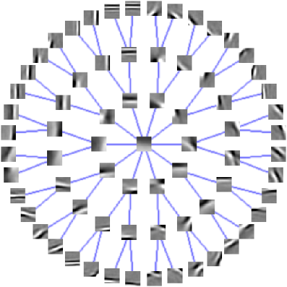
Figure 4: Learned dictionary with a tree structure of depth $4$. The root of the tree is in the middle of the figure. The branching factors at depths $1,2,3$ are respectively $10$, $2$, $2$. The dictionary is learned on $50,000$ patches of size $16\times 16$ pixels. Image taken from Ref. 11.

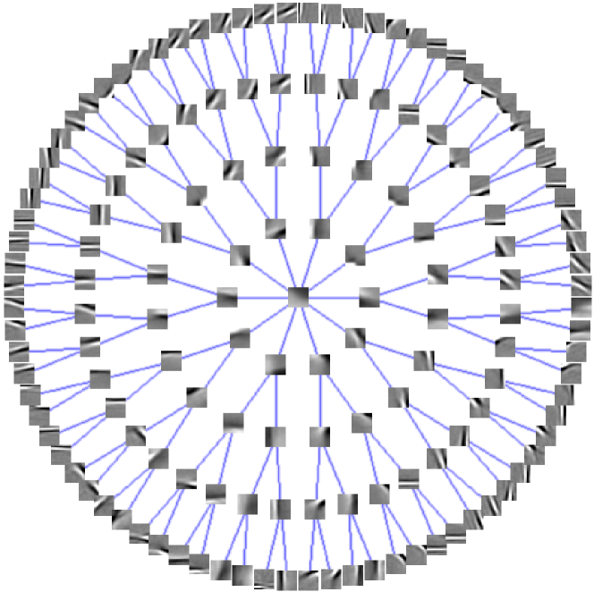
Figure 5: Learned dictionary with a tree structure of depth $5$. The root of the tree is in the middle of the figure. The branching factors at depths $1,2,3,4$ are respectively $10$, $2$, $2$, $2$. The dictionary is learned on $50,000$ patches of size $16\times 16$ pixels. Image taken from Ref. 11.

4.2 Topographic Dictionary Learning

In this experiment, we consider a database of $n=100\,000$ natural image patches of size $m=12\times 12$ pixels, for dictionaries of size $p=400$. As done in the context of independent component analysis (ICA)hyvarinen2 the dictionary elements are arranged on a two-dimensional grid, and we consider spatial dependencies between them. When learned on whitened natural image patches, this model called topographic ICA exhibits “Gabor-like” functions smoothly organized on the grid, which the authors call a topographic map. As shown in Ref. 20, such a result can be reproduced with a dictionary learning formulation, using a structured norm for $\psi$. Following their formulation, we organize the $p$ dictionary elements on a $\sqrt{p}\times\sqrt{p}$ grid, and consider $p$ overlapping groups that are $3\times 3$ or $4\times 4$ spatial neighborhoods on the grid (to avoid boundary effects, we assume the grid to be cyclic). We define $\psi$ as a sum of $\ell_{2}$-norms over these groups, since the $\ell_{\infty}$-norm has proven to be less adapted for this task. Another formulation achieving a similar effect was also proposed in Ref. 54 in the context of sparse coding with a probabilistic model.

As presented in Section 2.1, we consider a projected stochastic gradient descent algorithm for learning ${\mathbf{D}}$—that is, at iteration $t$, we randomly draw one signal ${\mathbf{y}}^{t}$ from the database ${\mathbf{Y}}$, compute a sparse code ${\boldsymbol{\alpha}}^{t}$ which is a solution of Eq. (1), and use the update rule of Eq. (6). In practice, to further improve the performance, we use a mini-batch, drawing $500$ signals at each iteration instead of one mairal7 . This approach mainly differs from Ref. 20 in the way the sparse codes ${\boldsymbol{\alpha}}^{t}$ are obtained. Whereas Ref. 20 uses a subgradient descent algorithm to solve them, we use the augmenting Lagrangian techniques presented in Section 3.2. The natural image patches we use are also preprocessed: They are first centered by removing their mean value, called DC component in the image processing literature, and whitened, as often done in the literature hyvarinen2 ; garrigues . The parameter $\lambda$ is chosen such that in average $\|{\mathbf{y}}^{i}-{\mathbf{X}}{\boldsymbol{\alpha}}^{i}\|_{2}\approx 0.4\|{\mathbf{y}}^{i}\|_{2}$ for every new patch considered by the algorithm, which yields visually interesting dictionaries. Examples of obtained results are shown on Figure 6 and 7, and exhibit similarities with the maps of topographic ICAhyvarinen2 .

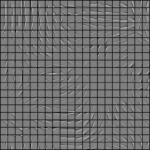
Figure 6: Topographic dictionaries with $400$ elements, learned on a database of $12\times 12$ whitened natural image patches with $3\times 3$ cyclic overlapping groups. Image taken from Ref. 13

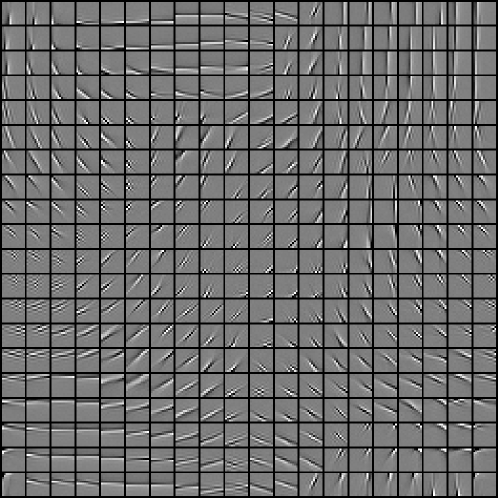
Figure 7: Topographic dictionaries with $400$ elements, learned on a database of $12\times 12$ whitened natural image patches with $4\times 4$ cyclic overlapping groups. Image taken from Ref. 13.

5 CONCLUSION

We have presented in this paper different convex penalties inducing both sparsity and a particular structure in the solution of an inverse problem. Whereas their most natural application is to model the structure of non-zero patterns of parameter vectors of a problem, associated for instance to physical constraints in bio-informatics, neuroscience, they also constitute a natural framework for learning structured dictionaries. We for instance observe that given an arbitrary structure, the dictionary elements can self-organize to adapt to the structure. The results obtained when applying these methods to natural image patches are intriguing, similarly as the ones produced by topographic ICA hyvarinen2 .

- (1) Zhao, P., Rocha, G., and Yu, B., “The composite absolute penalties family for grouped and hierarchical variable selection,” Annals of Statistics 37(6A), 3468–3497 (2009).
- (2) Jenatton, R., Audibert, J.-Y., and Bach, F., “Structured variable selection with sparsity-inducing norms,” tech. rep. (2009). Preprint arXiv:0904.3523v3.
- (3) Jacob, L., Obozinski, G., and Vert, J.-P., “Group Lasso with overlap and graph Lasso,” in [Proceedings of the International Conference on Machine Learning (ICML) ], (2009).
- (4) Huang, J., Zhang, Z., and Metaxas, D., “Learning with structured sparsity,” in [Proceedings of the International Conference on Machine Learning (ICML) ], (2009).
- (5) Baraniuk, R. G., Cevher, V., Duarte, M., and Hegde, C., “Model-based compressive sensing,” IEEE Transactions on Information Theory 56(4), 1982–2001 (2010).
- (6) Cehver, V., Duarte, M. F., Hedge, C., and Baraniuk, R. G., “Sparse signal recovery using Markov random fields,” in [Advances in Neural Information Processing Systems ], (2008).
- (7) He, L. and Carin, L., “Exploiting structure in wavelet-based Bayesian compressive sensing,” IEEE Transactions on Signal Processing 57(9), 3488–3497 (2009).
- (8) Turlach, B. A., Venables, W. N., and Wright, S. J., “Simultaneous variable selection,” Technometrics 47(3), 349–363 (2005).
- (9) Yuan, M. and Lin, Y., “Model selection and estimation in regression with grouped variables.,” Journal of the Royal Statistical Society: Series B 68, 49–67 (2006).
- (10) Obozinski, G., Taskar, B., and Jordan, M. I., “Joint covariate selection and joint subspace selection for multiple classification problems,” Statistics and Computing 20(2), 231–252 (2010).
- (11) Jenatton, R., Mairal, J., Obozinski, G., and Bach, F., “Proximal methods for hierarchical sparse coding,” Journal of Machine Learning Research 12, 2297–2334 (2011).
- (12) Mairal, J., Jenatton, R., Obozinski, G., and Bach, F., “Network flow algorithms for structured sparsity,” in [Advances in Neural Information Processing Systems ], (2010).
- (13) Mairal, J., Jenatton, R., Obozinski, G., and Bach, F., “Convex and network flow optimization for structured sparsity,” accepted with minor revision in the Journal of Machine Learning Research (JMLR), preprint arXiv:1104.1872 (2011).
- (14) Olshausen, B. A. and Field, D. J., “Sparse coding with an overcomplete basis set: A strategy employed by V1?,” Vision Research 37, 3311–3325 (1997).
- (15) Olshausen, B. A. and Field, D. J., “Emergence of simple-cell receptive field properties by learning a sparse code for natural images,” Nature 381, 607–609 (1996).
- (16) Engan, K., Aase, S. O., and Husoy, J. H., “Frame based signal compression using method of optimal directions (MOD),” in [Proceedings of the 1999 IEEE International Symposium on Circuits Systems ], 4 (1999).
- (17) Elad, M. and Aharon, M., “Image denoising via sparse and redundant representations over learned dictionaries,” IEEE Transactions on Image Processing 54, 3736–3745 (December 2006).
- (18) Mairal, J., Bach, F., Ponce, J., and Sapiro, G., “Online learning for matrix factorization and sparse coding,” Journal of Machine Learning Research 11, 19–60 (2010).
- (19) Mairal, J., Elad, M., and Sapiro, G., “Sparse representation for color image restoration,” IEEE Transactions on Image Processing 17, 53–69 (January 2008).
- (20) Kavukcuoglu, K., Ranzato, M., Fergus, R., and LeCun, Y., “Learning invariant features through topographic filter maps,” in [Proceedings of the IEEE Conference on Computer Vision and Pattern Recognition (CVPR) ], (2009).
- (21) Hyvärinen, A., Hoyer, P., and Inki, M., “Topographic independent component analysis,” Neural Computation 13(7), 1527–1558 (2001).
- (22) Candes, E. and Donoho, D. L., “New tight frames of curvelets and the problem of approximating piecewise images with piecewise edges,” Comm. Pure Appl. Math. 57, 219–266 (February 2004).
- (23) Donoho, D. L., “Wedgelets: Nearly minimax estimation of edges,” Annals of statistics 27, 859–897 (June 1998).
- (24) Mallat, S. and Pennec, E. L., “Bandelet image approximation and compression,” SIAM Multiscale Modelling and Simulation 4(3), 992–1039 (2005).
- (25) Mallat, S., [A Wavelet Tour of Signal Processing, Second Edition ], Academic Press, New York (September 1999).
- (26) Mairal, J., Bach, F., Ponce, J., Sapiro, G., and Zisserman, A., “Non-local sparse models for image restoration,” in [Proceedings of the IEEE International Conference on Computer Vision (ICCV) ], (2009).
- (27) Peyré, G., “Sparse modeling of textures,” Journal of Mathematical Imaging and Vision 34, 17–31 (May 2009).
- (28) Tibshirani, R., “Regression shrinkage and selection via the Lasso,” Journal of the Royal Statistical Society: Series B 58(1), 267–288 (1996).
- (29) Friedman, J., “Greedy function approximation: a gradient boosting machine,” Annals of Statistics 29(5), 1189–1232 (2001).
- (30) Weisberg, S., [Applied Linear Regression ], Wiley (1980).
- (31) Chen, S. S., Donoho, D. L., and Saunders, M. A., “Atomic decomposition by basis pursuit,” SIAM Journal on Scientific Computing 20, 33–61 (1999).
- (32) Mallat, S. and Zhang, Z., “Matching pursuit in a time-frequency dictionary,” IEEE Transactions on Signal Processing 41(12), 3397–3415 (1993).
- (33) Natarajan, B., “Sparse approximate solutions to linear systems,” SIAM journal on computing 24, 227 (1995).
- (34) Shapiro, J. M., “Embedded image coding using zerotrees of wavelet coefficients,” IEEE Transactions on Signal Processing 41(12), 3445–3462 (1993).
- (35) Aharon, M., Elad, M., and Bruckstein, A. M., “The K-SVD: An algorithm for designing of overcomplete dictionaries for sparse representations,” IEEE Transactions on Signal Processing 54, 4311–4322 (November 2006).
- (36) Lee, D. D. and Seung, H. S., “Algorithms for non-negative matrix factorization,” in [Advances in Neural Information Processing Systems ], 556–562 (2001).
- (37) Kushner, H. J. and Yin, G., [Stochastic Approximation and Recursive Algorithms and Applications ], Springer (2003).
- (38) Mairal, J., Sparse coding for machine learning, image processing and computer vision, PhD thesis, Ecole Normale Supérieure de Cachan (2010). http://tel.archives-ouvertes.fr/tel-00595312.
- (39) Bach, F., Jenatton, R., Mairal, J., and Obozinski, G., “Convex optimization with sparsity-inducing norms,” in [Optimization for Machine Learning ], Sra, S., Nowozin, S., and Wright, S. J., eds., MIT Press (2011). To appear.
- (40) Combettes, P. L. and Pesquet, J.-C., “Proximal splitting methods in signal processing,” in [Fixed-Point Algorithms for Inverse Problems in Science and Engineering ], Springer (2010).
- (41) Nesterov, Y., “Gradient methods for minimizing composite objective function,” tech. rep., Center for Operations Research and Econometrics (CORE), Catholic University of Louvain (2007).
- (42) Beck, A. and Teboulle, M., “A fast iterative shrinkage-thresholding algorithm for linear inverse problems,” SIAM Journal on Imaging Sciences 2(1), 183–202 (2009).
- (43) Brucker, P., “An O(n) algorithm for quadratic knapsack problems,” Operations Research Letters 3, 163–166 (1984).
- (44) Maculan, N. and de Paula, J. R. G. G., “A linear-time median-finding algorithm for projecting a vector on the simplex of ,” Operations Research Letters 8(4), 219–222 (1989).
- (45) Friedman, J., Hastie, T., and Tibshirani, R., “A note on the group Lasso and a sparse group Lasso,” tech. rep., Preprint arXiv:1001.0736 (2010).
- (46) Sprechmann, P., Ramirez, I., Sapiro, G., and Eldar, Y. C., “Collaborative hierarchical sparse modeling,” tech. rep. (2010). Preprint arXiv:1003.0400v1.
- (47) Bach, F., “Structured sparsity-inducing norms through submodular functions,” in [Adv. NIPS ], (2010).
- (48) Bertsekas, D. P. and Tsitsiklis, J. N., “Parallel and distributed computation: Numerical Methods,” (1989).
- (49) Tomioka, R., Suzuki, T., and Sugiyama, M., “Augmented Lagrangian methods for learning, selecting and combining features,” in [Optimization for Machine Learning ], Sra, S., Nowozin, S., and Wright, S. J., eds., MIT Press (2011). To appear.
- (50) Boyd, S., Parikh, N., Chu, E., Peleato, B., and Eckstein, J., “Distributed optimization and statistical learning via the alternating direction method of multipliers,” Foundations and Trends in Machine Learning 3(1), 1–122 (2011).
- (51) Qin, Z. and Goldfarb, D., “Structured sparsity via alternating directions methods,” tech. rep. (2011). preprint ArXiv:1105.0728.
- (52) Boyd, S. P. and Vandenberghe, L., [Convex Optimization ], Cambridge University Press (2004).
- (53) Martin, D., Fowlkes, C., Tal, D., and Malik, J., “A database of human segmented natural images and its application to evaluating segmentation algorithms and measuring ecological statistics,” in [Proceedings of the IEEE International Conference on Computer Vision (ICCV) ], (2001).
- (54) Garrigues, P. and Olshausen, B., “Group sparse coding with a laplacian scale mixture prior,” in [Advances in Neural Information Processing Systems ], (2010).