Super Bloch oscillations in the Peyrard-Bishop-Holstein model

Abstract

Recently, polarons in the Peyrard-Bishop-Holstein model under DC electric fields were established to perform Bloch oscillations, provided the charge-lattice coupling is not large. In this work, we study this model when the charge is subjected to an applied field with both DC and AC components. Similarly to what happens in the rigid lattice, we find that the carrier undergoes a directed motion or coherent oscillations when the AC field is resonant or detuned with respect to the Bloch frequency, respectively. The electric density current and its Fourier spectrum are also studied to reveal the frequencies involved in the polaron dynamics.

1 Introduction

In perfect crystals whose lattices generate a periodic potential, Bloch theorem predicts uniformly states extended over the whole system [2]. However, if a uniform electrical field $F$ is applied, in addition to this periodic potential, all states become spatially localized due to Bragg reflections [3, 4, 5]. In such a case, neglecting scattering effects, electron keep oscillating within a finite volume. The frequency $\omega_{B}$ and the amplitude $L_{B}$ of the oscillation can be established from semiclassical arguments [6, 7]. The former is usually known as Bloch frequency and it is proportional to the applied electric field $F$, namely $\omega_{B}=eFa/\hbar$, where $-e$ is the electron charge and $a$ refers to the lattice period along the field direction. This periodic motion takes place in real and in $k$ space, and it is known as Bloch oscillation (BO). Since scattering processes, due to phonons or defects for instance, destroy the coherence necessary to support BOs, its experimental detection is highly nontrivial. The first BOs were detected in semiconducting superlattices [8, 9, 10, 11, 12]. More recently, cold atoms and Bose-Einstein condensates (BECs) in optical lattices have been revealed as a very convenient scenario to observe BOs since scattering processes can be significantly reduced [13, 14, 15]. However, decoherence effects cannot be removed completely and should be taken into account from a theoretical point of view. For instance, in BECs the atom-atom interaction gives rise to well-known dynamical instabilities which can destroy the coherence required to observe stable BOs [16, 17, 18]. Still, there have been some experimental and theoretical proposals to avoid these undesirable effects [19, 20]. Also, in organic molecules, which are very flexible, the vibrations of the lattice are relevant and could rapidly degrade the electron quantum coherence. In this regard, the Peyrard-Bishop-Holstein (PBH) model of charge transport in DNA [21] was considered to demonstrate that polarons perform BOs even at realistic values of the carrier-lattice coupling [22].

In the last decade, a new interest in the dynamics of a quasiparticle affected not only by a DC field but also by a superimposed AC field has emerged [23, 24, 25, 26]. Remarkably, it was demonstrated experimentally that a weakly interacting BEC in a harmonically driven tilted potential can support directed transport or large amplitude oscillations of the wave function, depending on the driven frequency [27]. The latter are known as super Bloch oscillations (SBOs) and their characterizing parameters can also be described semiclassically [28]. In this work we use the PBH model to study how the introduction of the carrier-lattice interaction affects the dynamics of polarons in this scenario. We will also calculate the current density associated to the charge motion occurring under the applied fields and its Fourier spectrum to reveal the main frequencies involved in the polaron dynamics.

2 Model

The Hamiltonian of the PBH model can be written as

$${\cal H}={\cal H}_{\mathrm{lat}}+{\cal H}_{\mathrm{car}}+{\cal H}_{\mathrm{int}}\,.$$ (1)

The first term describes a one-dimensional anharmonic lattice according to the Peyrard-Bishop model [29]. A single degree of freedom $x_{n}$ is assigned to every site, taking into account its displacement from the equilibrium configuration. ${\cal H}_{\mathrm{lat}}$ for a homogeneous lattice reads

$${\cal H}_{\mathrm{lat}}=\sum_{n}^{N}\Big{[}\frac{1}{2}\,m\dot{x}^{2}_{n}+V(x_{n})+W(x_{n},x_{n-1})\Big{]}\,,$$ (2)

where $m$ is the mass of each site and $n=1,2,\ldots N$ labels the sites along the system. Two potential terms appear in this Hamiltonian, namely a local Morse potential $V(x_{n})$ and a nonlinear anharmonic coupling between nearest-neighbors $W(x_{n},x_{n-1})$

$$V_{M}(x_{n})=V_{0}\left(e^{-\alpha x_{n}}-1\right)^{2},$$ (3a)

$$W(x_{n},x_{n-1})=\frac{k}{4}\big{(}2+e^{-\beta(x_{n}+x_{n-1})}\big{)}\big{(}x_{n}-x_{n-1}\big{)}^{2}\ .$$ (3b)

For the sake of concreteness, the fitting parameters are chosen according to those obtained to reproduce experimental DNA melting curves within the Peyrard-Bishop model, $m=300\,$amu, $V_{0}=0.04\,$eV, $\alpha=4.45\,$Å^-1, $k=0.04\,$eV/Ų and $\beta=0.35\,$Å^-1 [30].

The charge carrier Hamiltonian ${\cal H}_{\mathrm{car}}$ in the unbiased lattice is expressed within the nearest-neighbor approximation as follows [31]

$${\cal H}_{\mathrm{car}}=-T\sum_{n}^{N}\left(a_{n}^{{\dagger}}a_{n+1}+a_{n+1}^{{\dagger}}a_{n}\right)\,,$$ (4)

where $T$ is the nearest-neighbor hopping and $a_{n}^{{\dagger}}$ and $a_{n}$ denotes the carrier creation and annihilation operators, respectively. Since there is not a common value for the parameter $T$ in the literature, we will take $T=0.1\,$eV hereafter as a good representative one [32, 33, 34].

The last term in (1) takes into account a Holstein-like carrier-lattice interaction as an on-site energy correction as follows [31]

$${\cal H}_{\mathrm{int}}=-\chi\sum_{n}^{N}x_{n}a_{n}^{{\dagger}}a_{n}\,.$$ (5)

Here $\chi$ denotes the carrier-lattice coupling constant. Ab-initio estimations of this coupling $\chi$ are scarce and therefore we will vary its magnitude in our numerical simulations.

In typical molecular systems it is possible to use a semiclassical approach due to the different time-scales of the charge and the lattice dynamics [35]. Thus, the dynamics of the carrier under a field with both DC and AC components such as $F(t)=F_{0}+F_{1}\sin(\omega t+\phi)$ can be studied by way of the following Schrödinger equation [21]

$$i\hbar\,\frac{d\psi_{n}}{dt}=-\big{[}U_{0}+U_{1}\sin(\omega t+\phi)\big{]}n\psi_{n}-T(\psi_{n+1}+\psi_{n-1})+\chi x_{n}\psi_{n}\ ,$$ (6)

where $\psi_{n}$ is the probability amplitude for the charge carrier located at the $n$th site. The parameters $U_{i}=eaF_{i}$ with $i=0,1$ are the energy terms associated to the applied electric fields $F_{0,1}$, $a$ being the period of the lattice (e.g. $a=3.4\,$Å in DNA). The last term in Eq. (6) describes the carrier-lattice coupling through the constant $\chi$ and the displacement $x_{n}$ from its equilibrium position. Newton’s equations of motion for the displacements $x_{n}$ become

$$m\,\frac{d^{2}x_{n}}{dt^{2}}=-V_{M}^{\prime}(x_{n})-W^{\prime}(x_{n},x_{n-1})-W^{\prime}(x_{n},x_{n+1})-\chi|\psi_{n}|^{2}\ ,$$ (7)

where the prime indicates differentiation with respect to $x_{n}$. In what follows we will take the stationary polaron of the unbiased system under consideration [31] as the initial condition for the integration of Eqs. (6) and (7) in a lattice subjected to the electric field $F(t)$.

3 Motion of the polaron in a biased system

In Ref. [27] the dynamics of a BEC under superposed DC and AC forces was observed experimentally. Later, the authors of Ref. [28] studied the wave packet dynamics under these conditions in a rigid lattice ($\chi=0$) by means of a semiclassical approach and numerical calculations. In both works it was reported that for a resonant AC field with frequency $\omega=\omega_{B}$, the wave function of the carrier performs a directed motion with oscillatory features with drift velocity depending on the phase $\phi$. On the contrary, if the frequency of the AC field is detuned with respect to $\omega_{B}$, the wave packet exhibits a beating effect called SBOs [27]. These two situations will be referred to as resonant and detuned cases hereafter. In this work, we will focus on two set of parameters as representative values of these two different situations, for several values of the carrier-lattice coupling.

First, we analyze how the polaron evolves when the field $F(t)=F_{0}+F_{1}\sin(\omega t+\phi)$ is applied. The time-domain evolution of the carrier wave packet obtained by direct integration of Eqs. (6) and (7) is shown in Fig. 1 for the resonant and the detuned cases, and $\chi=0.1$ and $0.3\,$eV/Å.

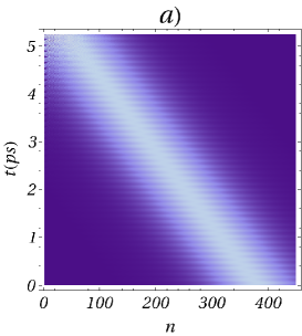
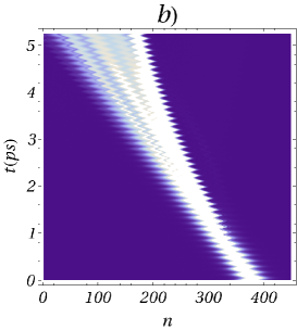
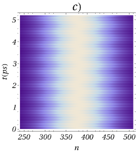
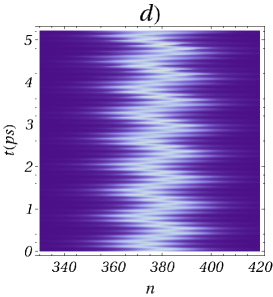
Figure 1: Modulus of the carrier wave function in a lattice of $N=750$ sites as a function of position and time with $F_{0}=10\,$meV/Å  $F_{1}=0.5F_{0}$ and $\chi=0.1\,$eV/Å (left panels) and $\chi=0.3\,$eV/Å (right panels). The two upper panels correspond to resonant cases with $\omega=\omega_{B}$ and $\phi=0$. The two lower panels correspond to detuned cases with $\omega=1.2\omega_{B}$ and $\phi=0$. Light and dark regions indicate nonzero and zero values, respectively.

Similarly to the case of the rigid lattice, the two upper panels of Fig. 1 (resonant cases with $\omega=\omega_{B}$) show the directed motion of the polaron as well as superimposed BOs. On the contrary, the two lower panels of Fig. 1 (detuned cases with $\omega=1.2\omega_{B}$) shows that the carrier perform SBOs. It is to be noticed that by increasing the strength of the carrier-lattice coupling the localization of the stationary states becomes larger and therefore the wave packet motion is more clearly observed (see Fig. 1d). We would like to stress that contrary to what happens in the rigid lattice [28], due to the nonlinear interactions the wave packet remains localized in time except for long time-scales if the carrier-lattice coupling is large, as seen in Fig. 1b).

The dynamics of the polaron can be monitored in more detail by means of the centroid of the carrier wave function $c(t)=\bar{n}(t)-\bar{n}(0)$ with $\bar{n}(t)=\sum_{n}n|\psi_{n}(t)|^{2}$. Similarly we define the dimensionless magnitude $l(t)=\xi(t)-\xi(0)$ with $\xi(t)=\sum_{n=1}^{N}n\,x_{n}(t)/a$ for the lattice displacements. We also study the Fourier transform of these magnitudes to reveal the frequencies involved in the dynamics of the polaron.

Figure 2 shows that $c(t)$ and $l(t)$ perform a directed motion with short-time-scale oscillations in a lattice of $N=2000$ sites. The Fourier spectrum $c(\omega)$ indicates that the main frequency of such oscillations is equal to $\omega_{B}=eaF_{0}/\hbar=51.67\,$THz (very weak peaks at multiples of $\omega_{B}$ are also found), while for $l(\omega)$ the Morse frequency $\omega_{M}=\sqrt{2V_{0}/m}=7.22\,$TH is the relevant one. Notice that the $\omega_{M}$ is the harmonic frequency of the small amplitude oscillations of a mass $m$ around the minimum of the Morse potential (3a).

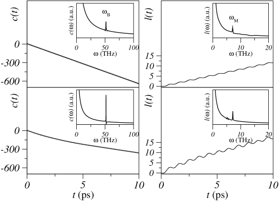
Figure 2: Centroid of the carrier wave function (left) and $l(t)$ (right) as a function of time in a lattice of $N=2000$ sites for $\omega=\omega_{B}$, $\phi=0$ and $\chi=0.1\,$eV/Å (upper panel) and $\chi=0.3\,$eV/Å (lower panel). Insets show the corresponding Fourier spectra.

The results corresponding to the detuned cases ($\omega=1.2\omega_{B}$) are shown in Fig. 3. $c(t)$ and $l(t)$ display a more complex dynamics and absence of directed motion. In the case of $c(t)$ the dynamics corresponds to the SBOs with a large period $2\pi/\Delta\omega$ defined by the detuning frequency $\Delta\omega=0.2\omega_{B}$ and a short period $2\pi/\omega_{B}$. In addition, in $c(\omega)$ we obtained other peaks which can be described with the full analytical solution of the centroid motion in the rigid lattice [23] [see the insets of the left panels of Fig. 3]. The main frequency involved in $l(t)$ is again the Morse frequency but now we also observe the occurrence of a smaller peak at the detuning frequency [see the insets of the right panels of Fig. 3]. Therefore, we come to the conclusion that in both situations the oscillations of the lattice and the carrier are almost decoupled, at least at moderate applied fields.

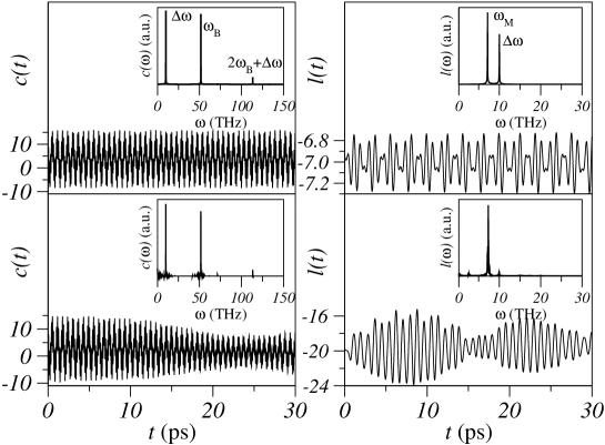
Figure 3: Same as in Fig. 2 but for detuned frequency ($\omega=1.2\omega_{B}$ and $\phi=0$) in a lattice of $N=750$.

4 Average current density

In view of the oscillating behavior of the carrier wave packet described in the previous section, it seems reasonable to expect that the electric current behaves in a similar way. Therefore, and since the current is a macroscopic magnitude which can be directly observed in experiments, we calculate the average current density $J(t)$ according to the following expression [21]

$$J(t)=\frac{\hbar e}{m_{c}Na^{2}}\sum_{n=1}^{N}\mathrm{Im}\big{[}\psi_{n}^{*}(\psi_{n+1}-\psi_{n-1})\big{]}\ ,$$ (8)

where $m_{c}$ is the mass of the carrier.

As in the previous section, we will consider different values of the carrier-lattice coupling for the representative resonant and detuned case. Typical results of our simulations are collected in Figs. 4 and 5. The left panels show the envelope of the average current density (8) over a long time interval while the insets display the short time behavior for two different values of the coupling constant $\chi=0.1\,$eV/Å and $\chi=0.3\,$eV/Å.

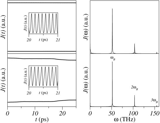
Figure 4: Left panels show the envelope of the average current density as a function of time in a lattice of $N=2000$ sites for the resonant case for $\omega=\omega_{B}$, $\phi=0$ and $\chi=0.1\,$eV/Å (upper panel) and $\chi=0.3\,$eV/Å (lower panel). Insets show the short time behavior of the average current density. The right panels show the corresponding Fourier transform of the average current density.

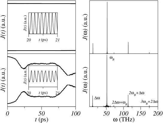
Figure 5: Same as in Fig. 4 but for detuned frequency ($\omega=1.2\omega_{B}$ and $\phi=0$) in a lattice of $N=750$.

The average current density displays a well-defined oscillatory behavior in both cases, whose relevant frequencies match perfectly those obtained from the centroid motion in Figs. 2 and 3. Notice that these frequencies are in agreement to those analytically predicted for the rigid lattice in all cases [23, 28]. We stress that the increase of the carrier-lattice coupling leads to a faster modulation of the average current density but, remarkably, the oscillations do not decay in time.

5 Conclusions

We have studied the dynamics of the carrier dynamics in the PBH model under superimposed DC and AC fields and found that it is similar to that found in the rigid lattice [27, 28]. The carrier-lattice coupling leads to a distortion of the initial shape of the wave packet at long times and to a faster modulation of the centroid motion. Still, the polaron display SBOs which do not decay in time when the driven frequency is detuned with respect to the Bloch frequency. The carrier is partially decoupled from the lattice, whose relevant frequency is not the Bloch frequency but the one associated to the Morse potential.

References

- [1]
- [2] W. A. Harrison, Solid State Theory. Dover Publications, (1980).
- [3] F. Bloch, Z. Phys. 52, 555 (1928).
- [4] C. Zener, Proc. R. Soc. London, Ser. A 145, 523 (1934).
- [5] D. H. Dunlap and V. M. Kenkre, Phys. Lett. A 127, 438 (1988).
- [6] L. Esaki and R. Tsu, IBM J. Res. Div. 14, 61 (1970).
- [7] N. W. Ashcroft, and N. D. Mermin, Solid State Physics. Saunders Colledge Publishers, New York, (1976).
- [8] J. Feldmann, K. Leo, J. Shah, D. A. B. Miller, J. E. Cunningham, T. Meier, G. von Plessen, A. Schulze, P. Thomas, and S. Schmitt-Rink, Phys. Rev. B 46, R7252 (1992).
- [9] C. Waschke, H. G. Roskos, R. Schwedler, K. Leo, H. Kurz, and K. Köhler, Phys. Rev. Lett. 70, 3319 (1993).
- [10] T. Dekorsy, P. Leisching, K. Köhler, and H. Kurz, Phys. Rev. B 50, R8106 (1994).
- [11] R. Martini, G. Klose, H. G. Roskos, H. Kurz, H. T. Grahn, and R. Hey, Phys. Rev. B 54, R14325 (1996).
- [12] F. Löser, Yu. A. Kosevich, K. Köhler, and K. Leo, Phys. Rev. B 61, R13373 (2000).
- [13] M. BenDahan, E. Peik, J. Reichel, Y. Castin, and C. Salomon, Phys. Rev. Lett. 76, 4508 (1996).
- [14] S. R. Wilkinson, C. F. Bharucha, K. W. Madison, Q. Niu, and M. G. Raizen, Phys. Rev. Lett. 76, 4512 (1996).
- [15] B. P. Anderson and M. A. Kasevich, Science 282, 1686 (1998).
- [16] G. Roati et al., Phys. Rev. Lett. 92, 230402 (2004).
- [17] L. Fallani, L. De Sarlo, J. E. Lye, M. Modugno, R. Saers, C. Fort, and M. Inguscio, Phys. Rev. Lett. 93, 140406 (2004).
- [18] A. Trombettoni and A. Smerzi, Phys. Rev. Lett. 86, 2353 (2001).
- [19] M. Gustavsson et al., Phys. Rev. Lett. 100, 080404 (2008).
- [20] C. Gaul, R. P. A. Lima, E. Díaz, C. A. Müller, and F. Domínguez- Adame, Phys. Rev. Lett. 102, 255303 (2009).
- [21] P. Maniadis, G. Kalosakas, K. Ø. Rasmunssen, and A. R. Bishop, Phys. Rev. E 72, 021912 (2005).
- [22] E. Díaz, R.P.A. Lima and F. Domínguez-Adame, Phys. Rev. B 78, 134303 (2008). Kolovsky10Thommen02Alberti09Ivanov08
- [23] A. R.. Kolovsky and H. J. Korsch, J. Siberian Federal University, Math. and Phys. 3, 311 (2010).
- [24] Q. Thommen, J. C. Garreau, and V. Zehnlé, Phys. Rev. A 65, 053406 (2002);
- [25] A. Alberti et al., Nature Phys. 5, 547 (2009).
- [26] V. V. Ivanov. A. Alberti, M. Schioppo, G. Ferrari, M. Artoni, M. L. Chiofalo, and G. M. Tino Phys. Rev. Lett. 100, 043602 (2008).
- [27] E. Haller et al., Phys. Rev. Lett. 104, 200403 (2010).
- [28] R. A. Cateano and M. L. Lyra, Phys. Lett. A 375, 2770 (2011).
- [29] M. Peyrard and A. R. Bishop, Phys. Rev. Lett. 62, 2755 (1989).
- [30] T. Dauxois and M. Peyrard, Phys. Rev. E 47, R44 (1993).
- [31] S. Komineas, G. Kalosakas, and A. R. Bishop, Phys. Rev. E 65, 061905 (2002).
- [32] Y. J. Yan and H. Zhang, J. Theor. Comp. Chem. 1, 225 (2002).
- [33] A. Voityuk, J. Jortner, M. Bixon, and N. Roesch, J. Chem. Phys. 114, 5614 (2002).
- [34] K. Senthilkumar, F. C. Grozema, C. F. Guerra, F. M. Bickelhaupt, F. D. Lewis, Y. A. Berlin, M. A. Ratner, and L. D. A. Siebbeles, J. Am. Chem. Soc. 127, 14894 (2005).
- [35] G. Kalosakas, S. Aubry, and G. P. Tsinronis, Phys. Rev. B 58, 3094 (1998).