Quantum fluctuations around black hole horizons in Bose-Einstein condensates

Abstract

We study several realistic configurations making it possible to realize an acoustic horizon in the flow of a one dimensional Bose-Einstein condensate. In each case we give an analytical description of the flow pattern, the spectrum of Hawking radiation and, the associated quantum fluctuations. Our calculations confirm that the non local correlations of the density fluctuations previously studied in a simplified model provide a clear signature of Hawking radiation also in realistic configurations. In addition we explain by direct computation how this non local signal relates to short range modifications of the density correlations.

I Introduction

During the last decade, it has been realized that Bose-Einstein condensates (BECs) were promising candidates for producing acoustic analogs of gravitational black holes, with possible experimental signature of the elusive Hawking radiation. The acoustic analogy had been proposed on a general setting by Unruh in 1981 Unruh , and its specific implementation using BECs has been first proposed by Garay et al., followed by many others HawkingBEC . We are now reaching a stage where experimental realizations and the study of these systems are possible Jeff10 and it is important to propose realistic configurations of acoustic black holes and possible signatures of Hawking radiation in BECs. Other experimental routes for observing analog Hawking radiation effects are based on non linear optical devices Phi08 or surface waves on moving fluids Rou10 . Note that this last option is restricted to the stimulated regime where the Hawking radiation results from a disturbance external to the system.

In this line, density correlations have been proposed in Ref. correlations as a tool making it possible to identify the spontaneous Hawking signal and to extract it from thermal noise. The physical picture behind this idea is the same as the one initially proposed by Hawking Hawking ; Par04 : quantum fluctuations can be viewed as constant emission and re-absorption of virtual particles. These particles can tunnel out near the event horizon and are then separated by the background flow (which is subsonic outside the acoustic black hole and supersonic inside), giving rise to correlated currents emitted away from the region of the horizon. In contrast to the gravitational case, the experimentalist is able to extract information from the interior of an acoustic black hole. It is thus possible to get insight on the Hawking effect by measuring a correlation signal between the currents emitted inside and outside the black hole. This two-body correlation signal appears to be poorly affected by the thermal noise and seems to be a more efficient measure of the Hawking effect than the direct detection of Hawking phonons (see Ref. Rec09 ).

In one dimensional (1D) flows of BECs, following a suggestion by Leonhardt et al. Leo03 , it is possible, within a Bogoliubov treatment of quantum fluctuations, to give a detailed account of the one and two-body Hawking signals. This idea was fully developed in Refs. Rec09 and Mac09 to obtain physical predictions for specific configurations. Ref. Rec09 focused on a schematic black hole configuration introduced in correlations and denoted as a “flat profile configuration” in the following: it consists of a uniform flow of a 1D BEC in which the two-body interaction is spatially modulated in order to locally modify the speed of sound in the system – forming a subsonic upstream region and a supersonic downstream one – although the velocity and the density of the flow remain constant. However, this type of flow, with a position dependent two-body interaction allowing an easy theoretical treatment, is only possible in presence of an external potential specially tailored so that the local chemical potential remains constant everywhere (see details in Sec. II.1). This makes the whole system quite difficult to realize experimentally.

In the present work we propose simpler sonic analogs of black holes for which a fully analytic theoretical treatment of the quantum correlations is still possible. We present a detailed account of the Bogoliubov treatment of quantum fluctuations in these settings and show that density correlations provide, also in these realistic configurations, a good evidence of the Hawking effect. We also discuss the recent work of Franchini and Kravtsov Fra09 who proposed an interesting scenario for explaining the peculiarities of the two-body density matrix $g^{(2)}$ in presence of an horizon. Elaborating on the similarities of $g^{(2)}$ with the level correlation function of non standard ensembles of random matrices Can95 , one can argue that the non local features of $g^{(2)}$ typical for Hawking radiation should be connected to a modification of its short range behavior. We spend some time for precisely discussing this point in the framework of the Bogoliubov description of the fluctuations. Our analytical study of the wave functions of the excitations makes it possible to obtain an non-ambiguous confirmation of this hypothesis.

The paper is organized as follows. In Sec. II we present three configurations allowing to realize an acoustic horizon in a 1D BEC. Then, in Sec. III, we discuss the practical implementation of the Bogoliubov approach to these non uniform systems. It appears convenient to describe the behavior of the excitations in the system in terms of a $S$-matrix, the properties of which are discussed in detail. This allows to describe the system using an approach valid for all possible black hole configurations. Within this framework, we study in Sec. IV the energy current associated to the Hawking effect and in Sec. V the density fluctuations pattern, putting special emphasis on its non local aspects. As discussed above we consider in detail their connection to short range modifications of the correlations. Finally we present our conclusions in Sec. VI. Some technical points are given in the appendices. In Appendix A we present the low energy behavior of the components of the $S$-matrix, in Appendix B we derive an expression for the energy current associated to the Hawking radiation and in Appendix C we precisely check that the two-body density matrix fulfills a sum rule connecting the short and long range behavior of the correlations in the system.

II The different black hole configurations

We work in a regime which has been denoted as “1D mean field” in Ref. Men02 . In this regime the system is described by a 1D Heisenberg field operator $\hat{\Psi}(x,t)$, solution of the Gross-Pitaevskii field equation. Writing $\hat{\Psi}(x,t)=\hat{\Phi}(x,t)\exp(-{\rm i}\mu t/\hbar)$ this reads

$${\rm i}\hbar\,\partial_{t}\hat{\Phi}=-\frac{\hbar^{2}}{2m}\partial^{2}_{x}\hat{\Phi}+[U(x)+g\hat{n}-\mu]\hat{\Phi}.$$ (1)

In Eq. (1) $\mu$ is the chemical potential, fixed by boundary conditions at infinity; $\hat{n}(x,t)=\hat{\Phi}^{\dagger}\hat{\Phi}$ is the density operator and $U(x)$ is an external potential (its precise form depends on the black hole configuration considered). $g$ is a non linear parameter which depends on the two-body interaction within the BEC and on the transverse confinement. Both are possibly position dependent. For a repulsive effective two-body interaction described by a positive 3D $s$-wave scattering length $a$ and for a transverse harmonic trapping of pulsation $\omega_{\perp}$, one has $g=2a\hbar\omega_{\perp}$ Ols98 . In the flat profile configuration of Ref. correlations $g$ depends on the position $x$ (see Sec. II.1), whereas it is constant in the realistic configurations introduced below and respectively denoted as delta peak (Sec. II.2) and waterfall (Sec. II.3) configurations.

Within the Bogoliubov approach, in the quasi-condensate regime, the quantum field operator $\hat{\Phi}$ is separated in a classical contribution $\Phi$ describing the background flow pattern plus a small quantum correction $\hat{\psi}$. In all the configurations we consider, the flow pattern is stationary and one thus writes

$$\hat{\Phi}(x,t)=\Phi(x)+\hat{\psi}(x,t),$$ (2)

$\Phi(x)$ being the solution of the classical stationary Gross-Pitaevskii equation

$$\mu\Phi=-\frac{\hbar^{2}}{2m}\partial^{2}_{x}\Phi+[U(x)+g|\Phi|^{2}]\Phi.$$ (3)

A black hole configuration corresponds to a disymmetry between the upstream flow and the downstream one, separated by the event horizon. In the following we use a subscript “$u$” for upstream and “$d$” for downstream. The downstream region corresponds to $x>0$ and is supersonic. The upstream region corresponds to $x<0$ and is subsonic (see, however, the remark at the end of Sec. II.3). We thus write

$$\Phi(x)=\left\{\begin{array}[]{lcl}\sqrt{n_{u}}\exp({\rm i}k_{u}x)\phi_{u}(x)&\mbox{for}&x<0,\\ \sqrt{n_{d}}\exp({\rm i}k_{d}x)\phi_{d}(x)&\mbox{for}&x>0.\end{array}\right.$$ (4)

In (4) $\lim_{x\to-\infty}|\phi_{u}(x)|=1$ and $\lim_{x\to+\infty}|\phi_{d}(x)|=1$, so that $n_{u}$ and $n_{d}$ are respectively the upstream and downstream asymptotic densities. Also $k_{\alpha}=mV_{\alpha}/\hbar$ ($\alpha=u$ or $d$), where $V_{u}$ is the asymptotic upstream flow velocity and $V_{d}$ the asymptotic downstream one ($V_{u}$ and $V_{d}$ are both positive).

In the following we denote the asymptotic velocities of sound as $c_{u}$ and $c_{d}$ with $mc_{\alpha}^{2}=g_{\alpha}n_{\alpha}$, where $g_{u,d}=\lim_{x\to-\infty,+\infty}g(x)$ (we keep the possibility of a position dependent $g$ coefficient in order to treat the flat profile configuration of Ref. correlations ). We also introduce the healing lengths $\xi_{\alpha}=\hbar/(mc_{\alpha})$ and the Mach numbers $\mathpzc{m}_{\alpha}=V_{\alpha}/c_{\alpha}$. In a black hole configurations $\mathpzc{m}_{u}<1$ and $\mathpzc{m}_{d}>1$.

Denoting $U_{u,d}=\lim_{x\to-\infty,+\infty}U(x)$ one gets from (3) and (4)

$$\frac{\hbar^{2}k^{2}_{\alpha}}{2m}+U_{\alpha}+g_{\alpha}n_{\alpha}=\mu\quad\mbox{and}\quad n_{u}V_{u}=n_{d}V_{d}.$$ (5)

The first of these equations corresponds to the equality of the asymptotic chemical potentials and is required for a stationary flow; the second equation corresponds to current conservation in a stationary flow.

The precise form of the flow pattern is specified by the functions $\phi_{u}(x)$ and $\phi_{d}(x)$ which depend on the configuration considered. In all the configurations treated below $\phi_{d}(x)$ is a constant of the form

$$\phi_{d}(x)=\exp({\rm i}\beta_{d}),$$ (6)

meaning that the downstream flow pattern is flat with a constant density and velocity. The value of $\beta_{d}$ depends on the configuration considered. As for the upstream flow pattern, the stationary flow condition imposes $\lim_{x\to-\infty}\phi_{u}(x)=\exp({\rm i}\beta_{u})$, where $\beta_{u}$ is a constant.

After having defined the notations and the common aspects of all the flow patterns, we now give the precise value of the configuration-dependent parameters.

II.1 Flat profile configuration

We recall here the value of the parameters in the flat profile configuration studied in correlations ; Rec09 . In this case the $\phi_{\alpha}$ functions of Eq. (4) assume a very simple value: $\phi_{u}(x)=\phi_{d}(x)=1$ (and thus $\beta_{u}=\beta_{d}=0$). One has

$$U(x)=\left\{\begin{array}[]{lcl}U_{u}&\mbox{for}&x<0,\\ U_{d}&\mbox{for}&x>0,\end{array}\right.$$ (7)

and

$$g(x)=\left\{\begin{array}[]{lcl}g_{u}&\mbox{for}&x<0,\\ g_{d}&\mbox{for}&x>0,\end{array}\right.$$ (8)

chosen so that a flow with $V_{u}=V_{d}\equiv V_{0}$ and $n_{u}=n_{d}\equiv n_{0}$ is solution of Eqs. (3) and (5); i.e., Eq. (4) reduces to $\Phi(x)=\sqrt{n_{0}}\exp({\rm i}k_{0}x)$ for all $x$ ($k_{0}=mV_{0}/\hbar$). This imposes

$$\frac{c_{d}}{c_{u}}=\frac{\mathpzc{m}_{u}}{\mathpzc{m}_{d}}=\frac{\xi_{u}}{\xi_{d}},$$ (9)

and

$$g_{u}n_{0}+U_{u}=g_{d}n_{0}+U_{d}.$$ (10)

We finally note that in the flat profile configuration one has $c_{d}<V_{d}=V_{u}<c_{u}$.

In the numerical simulations of Refs. correlations ; Mac09 , a generalization of this step-like configuration has been used; one considers smooth $U(x)$ and $g(x)$ functions imposing the continuous version of (10): $g(x)n_{0}+U(x)=\rm{C^{st}}$. The theoretical approach is the same as in Ref. Rec09 but the Bogoliubov-de Gennes equations [Eq. (19) below] have to be solved numerically whereas the step-like configuration characterized by Eqs. (7) and (8) allows for an analytical treatment.

The flat profile configuration can be numerically implemented in a dynamical way as explained in Ref. correlations . However, it is fair to say that the corresponding experiment seems rather difficult to realize. Moreover the flat profile configuration is very sensitive to the total atom number, a quantity which is not easily controlled experimentally. Besides a local monitoring of $g(x)$ has not yet been demonstrated. There are the reasons why in the following subsections we introduce two new types of sonic horizon which can be implemented experimentally more easily.

II.2 Delta peak configuration

In this configuration the non linear coefficient $g$ is constant and the external potential is a repulsive delta peak: $U(x)=\Lambda\delta(x)$, with $\Lambda>0$. It has been noticed in Ref. Leb01 that one can find in this case a stationary profile with a flow which is subsonic far upstream and supersonic downstream (i.e., a black hole configuration). The upstream flow corresponds to a portion of a dark soliton profile. More precisely, for $x<0$, one has

$$\phi_{u}(x)=\cos\theta\,\tanh\left(\frac{x-x_{0}}{\xi_{u}}\cos\theta\right)-{\rm i}\sin\theta,$$ (11)

where $\sin\theta=\mathpzc{m}_{u}$, and one can restrict oneself to $\theta\in[0,\pi/2]$ (then $\beta_{u}=\pi+\theta$). As is also the case for the other configurations studied in the present work, the downstream flow has a constant density and velocity [cf. Eq. (6)]. The typical profile is displayed in Fig. 1.

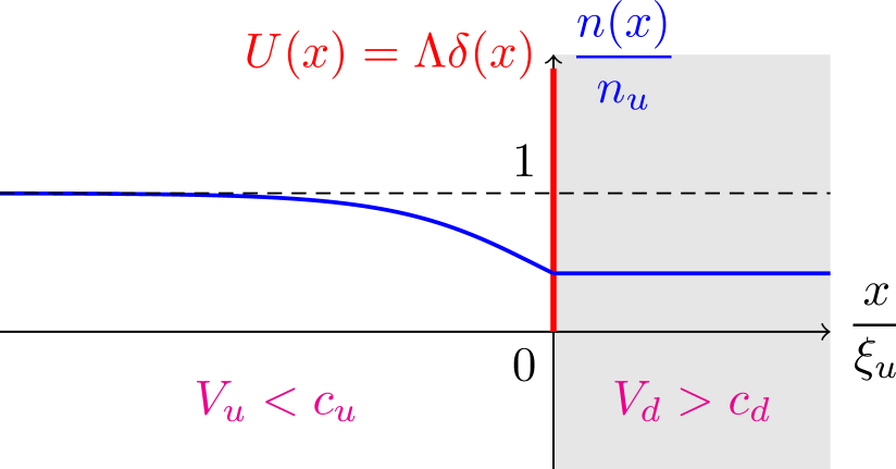
Figure 1: (Color online) Density profile in the delta peak configuration. The flow is directed toward positive $x$. The delta potential is represented by a (red) vertical straight line. The density in the upstream region ($x<0$) is a portion of a dark soliton (see the text). The region $x>0$ is supersonic. It is shaded in the plot for recalling that it corresponds to the interior of the equivalent black hole. We keep this convention in Figs. 2, 3 and 4.

Once $\mathpzc{m}_{u}=V_{u}/c_{u}$ is fixed ($<1$) all the other parameters of the flow are determined by Eqs. (5). Defining $y=\frac{1}{2}\left(-1+\sqrt{1+8/\mathpzc{m}_{u}^{2}}\right)$ one gets

$$\frac{n_{u}}{n_{d}}=\frac{V_{d}}{V_{u}}=y,\quad\frac{\mathpzc{m}_{d}}{\mathpzc{m}_{u}}=y^{\frac{3}{2}},\quad\frac{c_{d}}{c_{u}}=\frac{1}{\sqrt{y}}=\frac{\xi_{u}}{\xi_{d}}.$$ (12)

By imposing continuity of the wave function [$\Phi(0)=\sqrt{n_{d}}\exp({\rm i}\beta_{d})=\sqrt{n_{u}}\,\phi_{u}(0)$] and the appropriate matching of its first derivative [$\partial_{x}\Phi(0^{+})-\partial_{x}\Phi(0^{-})=2m\hbar^{-2}\Lambda\Phi(0)$] one gets

$$\sin\beta_{d}=-\mathpzc{m}_{u}\sqrt{y},$$ (13)

$$\frac{x_{0}}{\xi_{u}}=\frac{1}{\cos\theta}\tanh^{-1}\left(\sqrt{\frac{y-1}{2}}\tan\theta\right),$$ (14)

and also

$$\Lambda=\frac{\lambda\hbar^{2}}{m\xi_{u}}\quad\mbox{with}\quad\lambda=\mathpzc{m}_{u}\left(\frac{y-1}{2}\right)^{\frac{3}{2}}.$$ (15)

In this configuration one has $V_{u}<c_{d}<c_{u}<V_{d}$ which corresponds to a black hole type of horizon. Related work for a double barrier configuration recently appeared in Zap11 .

Note that the flow depicted in Fig. 1 corresponds to a very specific case in the parameter space spanned by the intensity of the delta potential and the flow velocities, which is on the verge of becoming time dependent (see Ref. Leb01 ). This is reflected by the fact that, for this configuration, $\mathpzc{m}_{u}$ and $\mathpzc{m}_{d}$ cannot be fixed independently (in contrast to what occurs for the flat profile case). One might thus legitimately expect to face a fine tuning problem to experimentally fulfill all the required boundary conditions (12) (13), (14) and (15). One could also argue that a delta potential is non standard and that the specific structure of the flow pattern displayed in Fig. 1 would disappear for a more realistic potential. However, it is shown in Ref. Car11 that this configuration can be rather easily obtained by launching a 1D condensate on a localized obstacle (not necessarily a delta peak). In this case, there exists a sizable range of parameters where, after ejection of an upstream dispersive shock wave, the long time flow pattern becomes of the type illustrated in Fig. 1.

II.3 Waterfall configuration

In this configuration the two-body interaction is constant and the external potential is a step function of the form $U(x)=-U_{0}\Theta(x)$, where $\Theta$ is the Heaviside function (and $U_{0}>0$). In this case, a stationary profile with a flow which is subsonic upstream and supersonic downstream, i.e., a black hole configuration, has been identified in Ref. Leb03 . The upstream profile is, as for the delta peak configuration, of the form (11), with here $x_{0}=0$, i.e., the upstream profile is exactly one half of a dark soliton. The corresponding density profile is displayed in Fig. 2.

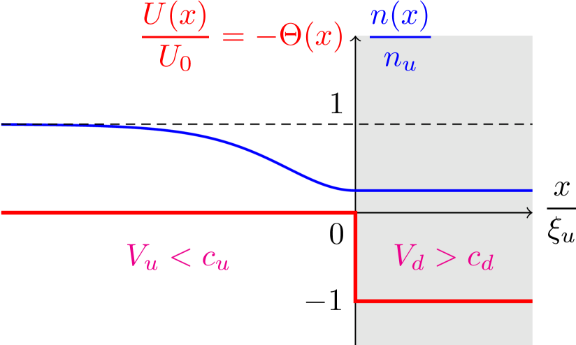
Figure 2: (Color online) Same as Fig. 1 for the waterfall configuration.

The equalities (5) and the continuity of the order parameter at the origin impose here

$$\frac{V_{d}}{V_{u}}=\frac{n_{u}}{n_{d}}=\frac{1}{\mathpzc{m}_{u}^{2}}=\mathpzc{m}_{d}=\left(\frac{\xi_{d}}{\xi_{u}}\right)^{2}=\left(\frac{c_{u}}{c_{d}}\right)^{2},$$ (16)

$\exp({\rm i}\beta_{d})=-{\rm i}$, and

$$\frac{U_{0}}{gn_{u}}=\frac{\mathpzc{m}_{u}^{2}}{2}+\frac{1}{2\mathpzc{m}_{u}^{2}}-1.$$ (17)

In this configuration one has $V_{u}=c_{d}<c_{u}<V_{d}$ which corresponds to a black hole type of horizon.

The remark given at the end of Sec. II.2 is here also in order: there might be a fine tuning problem for verifying Eqs. (16) and (17). Although we did not perform here the time dependent analysis done in Ref. Car11 for the delta peak configuration, we believe that, also in the present case, it is possible to dynamically reach the stationary configuration depicted in Fig. 2. This is supported by the experimental results presented by the Technion group Jeff10 who studied a very similar configuration (with the additional complication of the occurrence of a white hole horizon). These results show no important time dependent features near the black hole horizon and we are thus led to consider that the stationary waterfall configuration of the type illustrated in Fig. 2 is stable and can be reached experimentally.

We make here a remark which is also relevant for the delta peak configuration: the precise location of the sonic horizon is not well defined. In both configurations (waterfall or delta peak) one may define a local sound velocity, and the point where the local flow velocity exceeds the local speed of sound can be chosen as the location of the sonic horizon. Then one finds that the sonic horizon is located slightly upstream the interface $x=0$ (in the waterfall configuration for instance, at $x=0$ the local flow velocity is already $\mathpzc{m}_{u}^{-2}$ times larger than the local sound velocity). However, the local sound velocity is an approximate concept, only rigorously valid in regimes where the BEC density varies over typical length scales much larger than the healing length. This is not the case in the waterfall and delta peak configurations near $x=0$ and, as a result, the concept of sonic horizon is ill defined. In the fully quantum treatment presented below we do not use this concept: the important point for our analysis is simply that the upstream flow velocity is asymptotically (i.e., when $x\to-\infty$) larger than $c_{u}$. Hence, for preciseness we do not state that the upstream flow is subsonic, but that it is asymptotically subsonic.

III Fluctuations around the stationary profile

In this section we establish a basis set in each of the flow regions (upstream and downstream) which will be used in Sec. III.6 for describing the quantum fluctuations in the system. The simplest way to obtain this basis set is to start from expression (2), with $\Phi(x)$ given by (4), and to treat $\hat{\psi}(x,t)$ as a small time dependent classical field, denoted as $\psi(x,t)$ in the present section, with $\Phi(x)+\psi(x,t)$ solution of the classical version of (1). One looks for a normal mode of the form

$$\psi(x,t)=\mathrm{e}^{{\rm i}k_{\alpha}x}\left[\bar{u}_{\alpha}(x,\omega)\mathrm{e}^{-{\rm i}\omega t}+\bar{w}_{\alpha}^{*}(x,\omega)\mathrm{e}^{{\rm i}\omega t}\right],$$ (18)

with $\alpha=u$ for $x<0$ and $\alpha=d$ for $x>0$. $\Phi(x,t)$ defined by Eqs. (2) and (18) describes small oscillations with pulsation $\omega$ of the order parameter around the ground state $\Phi(x)$. In the following we drop the $\omega$ dependence of functions $\bar{u}_{\alpha}$ and $\bar{w}_{\alpha}$ for legibility. We also write $X_{\alpha}=x/\xi_{\alpha}$ (and then $k_{\alpha}x=\mathpzc{m}_{\alpha}X_{\alpha}$). Linearizing the Gross-Pitaevskii equation, one gets at first order in $\psi$:

$$\varepsilon_{\alpha}\begin{pmatrix}\bar{u}_{\alpha}\\ \bar{w}_{\alpha}\end{pmatrix}=\mathcal{L}_{\alpha}\begin{pmatrix}\bar{u}_{\alpha}\\ \bar{w}_{\alpha}\end{pmatrix},$$ (19)

with

$$\mathcal{L}_{\alpha}=\begin{pmatrix}H_{\alpha}-{\rm i}\mathpzc{m}_{\alpha}\partial_{X_{\alpha}}&\phi_{\alpha}^{2}\\ -(\phi_{\alpha}^{*})^{2}&-H_{\alpha}-{\rm i}\mathpzc{m}_{\alpha}\partial_{X_{\alpha}}\end{pmatrix},$$ (20)

where $\varepsilon_{\alpha}=\hbar\omega/(g_{\alpha}n_{\alpha})$ and $H_{\alpha}=-\frac{1}{2}\partial^{2}_{X_{\alpha}}+2|\phi_{\alpha}|^{2}-1$. Hence, the column vector formed by $\bar{u}_{\alpha}$ and $\bar{w}_{\alpha}$ is an eigen-vector of the so called Bogoliubov-de Gennes Hamiltonian $\mathcal{L}_{\alpha}$.

The present section is organized as follows. We first consider solutions of (19) for $X_{\alpha}\in\mathbb{R}$ in Sec. III.1. We give the expression of these solutions in sections III.2 and III.3, specifying only what we need for the following step: that is, for $\alpha=d$, we only display the form of the solution when $x>0$, and for $\alpha=u$, we only display the form of the solution when $x<0$. The most general fluctuation of pulsation $\omega$ is a linear combination of eigen-modes for the upstream region glued at $x=0$ with a linear combination of the downstream eigen-modes. We explain how this matching is done in Sec. III.4. Finally, in Sec. III.5, we specify the form of the scattering modes which are the appropriate modes used for quantizing the fluctuations in Sec. III.6.

III.1 Properties of the eigen-functions of the Bogoliubov-de Gennes equation

The relevant eigen-functions of (19) are of the form

$$\begin{pmatrix}\bar{u}_{\ell}(x)\\ \bar{w}_{\ell}(x)\end{pmatrix}=\mathrm{e}^{{\rm i}Q_{\ell}X_{\alpha}}\begin{pmatrix}{\cal U}_{\ell}(x)\\ {\cal W}_{\ell}(x)\end{pmatrix},$$ (21)

where the functions ${\cal U}_{\ell}(x)$ and ${\cal W}_{\ell}(x)$ are constant for $|x|\to\infty$ (more precisely in the domain where $\phi_{\alpha}$ is constant). Their exact form will be specified later [Eqs. (27) and (32)]. In Eq. (21) the $Q_{\ell}$’s are the dimensionless wave vectors of the Bogoliubov modes, solutions of

$$(\varepsilon_{\alpha}-\mathpzc{m}_{\alpha}Q)^{2}=\omega_{\rm\scriptscriptstyle B}^{2}(Q),$$ (22)

where

$$\omega_{\rm\scriptscriptstyle B}(Q)=Q\sqrt{1+\frac{Q^{2}}{4}}$$ (23)

is the Bogoliubov dispersion relation in a condensate at rest (written in dimensionless form). Note that $Q_{\ell}$ – solution of (22) – is sometimes complex; this fact is taken into account in the following. In particular, for $\alpha=u$ ($\alpha=d$) one should discard values of the wave vector such that ${\rm Im}(Q_{\ell})>0$ (${\rm Im}(Q_{\ell})<0$). This corresponds to eliminating the evanescent channels in the region where they are divergent. For instance, a mode with $\mbox{Im}(Q_{\ell})<0$ diverges when $x\to+\infty$, which will correspond to the supersonic region (labeled $d$) in the following, and we thus discard it. The dispersion relations and the different real wave vectors are displayed in Fig. 3.

The index $\alpha$ of Eq. (18) is specified to $\ell$ in (21) for identifying the branch of the dispersion relation to which the considered excitation pertains. For precise notations, $\ell$ is taken as a double index, because it is clear from (22) that the values of the wave vectors are not the same in the subsonic and supersonic regions, i.e., they depend on $\alpha$. Specifically, when $\alpha=u$, $\ell\in\{u|{\rm in},u|{\rm out},u|{\rm eva}\}$. When $\alpha=d$, there are two cases, depending if $\omega$ is lower or greater than a certain threshold $\Omega$. If $\omega<\Omega$, $\ell\in\{d1|{\rm in},d1|{\rm out},d2|{\rm in},d2|{\rm out}\}$ and when $\omega>\Omega$, $\ell\in\{d1|{\rm in},d1|{\rm out},d|{\rm eva}\}$.

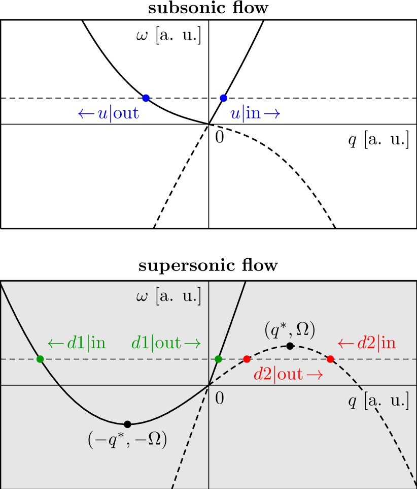
Figure 3: (Color online) Dispersion relation (22). In each plot the horizontal dashed line is fixed by the chosen value of $\omega$. The $q_{\ell}(\omega)$’s are the corresponding abscissae. Only the real eigen-modes are represented; their denomination is explained in the text; their direction of propagation (left or right) is represented by an arrow. The part of the dispersion relation corresponding to negative norm states (see the text) is represented with a dashed line. The upper plot corresponds to a subsonic flow. The lower one corresponds to a supersonic flow; it is shaded in order to recall that it describes the situation inside the black hole.

We have chosen to label the real eigen-modes as “in” (such as $d1|{\rm in}$ for instance) or “out” (such as $u|{\rm out}$) depending if their group velocity [its explicit expression is given below, Eq. (29)] points toward the horizon (for the “in” modes) or away from the horizon (for the “out” modes) in a black hole configuration, i.e., with a subsonic region at left of the horizon, the supersonic region being at the right. The wave vectors labeled $u|{\rm eva}$ and $d|{\rm eva}$ are complex and correspond to evanescent channels (as explained above, one selects the complex $Q_{\ell}$’s which describe waves decaying at infinity).

The threshold $\Omega$ appearing in the lower plot of Fig. 3 is reached only for a supersonic flow, for a wave vector $q^{*}$ such that

$$q^{*}\xi_{d}=Q^{*}_{d}=\left(-2+\frac{\mathpzc{m}_{d}^{2}}{2}+\frac{\mathpzc{m}_{d}}{2}\sqrt{8+\mathpzc{m}_{d}^{2}}\right)^{\frac{1}{2}}.$$ (24)

The existence of this threshold is a consequence of the behavior of the large momentum part of the dispersion relation $\omega_{\rm\scriptscriptstyle B}(Q)$ of a condensate at rest. More precisely, the part of the dispersion relation which shows a local maximum in the supersonic region corresponds to the particular solution of (22) where $\varepsilon_{d}-\mathpzc{m}_{d}Q=-\omega_{\rm\scriptscriptstyle B}(Q)$. At $Q=Q^{*}_{d}$ one has exactly $\partial\omega_{\rm\scriptscriptstyle B}/\partial Q=\mathpzc{m}_{d}$, and for $Q>Q^{*}_{d}$, one has $\partial\omega_{\rm\scriptscriptstyle B}/\partial Q>\mathpzc{m}_{d}$. Hence the part of the spectrum with $Q>Q^{*}_{d}$ corresponds to excitations whose group velocity in the frame where the condensate is at rest ($\partial\omega_{\rm\scriptscriptstyle B}/\partial Q$) is larger than the flow velocity $\mathpzc{m}_{d}$ (we use here dimensionless quantities). One can have $\partial\omega_{\rm\scriptscriptstyle B}/\partial Q>\mathpzc{m}_{d}>1$ only because the dispersion relation (23) grows faster than linear at large $Q$. We will see in Sec. IV that the corresponding waves play an important role in the zero temperature Hawking signal.

It is easy to verify that, if $(\bar{u}_{\alpha},\bar{w}_{\alpha})$ is a solution of (19) associated to an eigen-energy $\varepsilon_{\alpha}$, then $(\bar{w}_{\alpha}^{*},\bar{u}_{\alpha}^{*})$ is also a solution of (19), now associated to eigen-energy $-\varepsilon_{\alpha}$. Besides, from expression (18), one sees that both solutions describe the same perturbation of the condensate. As a result, one can always select eigen-modes with positive values of $\varepsilon_{\alpha}=\hbar\omega/(g_{\alpha}n_{\alpha})$, and in all the following we chose $\omega\in\mathbb{R}^{+}$.

One may also notice that the above symmetry of the wave function is associated to the normalization of the eigen-modes. For instance, it is clear that the symmetry operation changes the sign of $|{\cal U}_{\ell}|^{2}-|{\cal W}_{\ell}|^{2}$ and one can show by simple algebraic manipulations that, for real $Q_{\ell}$, the sign of $|{\cal U}_{\ell}|^{2}-|{\cal W}_{\ell}|^{2}$ is the same as the sign of $\varepsilon_{\alpha}-\mathpzc{m}_{\alpha}Q_{\ell}$. In the following we denote the eigen-modes for which $|{\cal U}_{\ell}|^{2}-|{\cal W}_{\ell}|^{2}>0$ as having a positive normalization (for a recent discussion of this point see see, e.g. Ref. Bar10 , as well as Refs. BR86 ; Fet98 ). In Fig. 3 their dispersion relation is represented with a solid line, whereas the eigen-modes with negative normalization are represented with a dashed line. In particular, in the supersonic region, the $d2|{\rm in}$ and $d2|{\rm out}$ channels have negative norm for $0<\omega<\Omega$.

It was shown in Dal96 that each eigen-vector of equation (19) is associated with a conserved (i.e., $x$ independent) current $J_{\ell}$. We show below (see Sec. IV) how $J_{\ell}$ relates to the energy current in the system. $J_{\ell}$ is zero for complex $Q_{\ell}$ (evanescent waves do not carry any current); this can be proven directly in our specific case, but we do not display the proof here. For real $Q_{\ell}$ one gets

$$J_{\ell} =c_{\alpha}\Big{[}(Q_{\ell}+\mathpzc{m}_{\alpha})|{\cal U}_{\ell}|^{2}+(Q_{\ell}-\mathpzc{m}_{\alpha})|{\cal W}_{\ell}|^{2}\Big{]}$$

$$+c_{\alpha}{\rm Im}\left({\cal U}_{\ell}^{*}\partial_{X_{\alpha}}{\cal U}_{\ell}+{\cal W}_{\ell}^{*}\partial_{X_{\alpha}}{\cal W}_{\ell}\right).$$ (25)

Going back to dimensioned quantities and using the $\bar{u}_{\ell}$ and $\bar{w}_{\ell}$ functions, this reads

$$J_{\ell}=\frac{\hbar}{2m}\Big{[}\bar{u}^{*}_{\ell}(k_{\alpha}-{\rm i}\partial_{x})\bar{u}_{\ell}-\bar{w}^{*}_{\ell}(k_{\alpha}+{\rm i}\partial_{x})\bar{w}_{\ell}\Big{]}+{\rm c.c.},$$ (26)

where “c.c.” stands for “complex conjugate”.

III.2 Downstream region: $x>0$

We recall that in this region the flow is supersonic and that the eigen-vectors are labeled with an index $\ell\in\{d1|{\rm in},d1|{\rm out},d2|{\rm in},d2|{\rm out}\}$ when $\omega<\Omega$ and $\ell\in\{d1|{\rm in},d1|{\rm out},d|{\rm eva}\}$ when $\omega>\Omega$.

Here $\phi_{d}^{2}$ appearing in Eq. (20) does not depend on $x$ and is equal to $\exp(2{\rm i}\beta_{d})$ remarque . This implies that the functions ${\cal U}_{\ell}$ and ${\cal W}_{\ell}$ are also $x$ independent. One finds

$$\begin{pmatrix}{\cal U}_{\ell}\\ {\cal W}_{\ell}\end{pmatrix}=\frac{1}{{\cal C}_{\ell}}\begin{pmatrix}(Q_{\ell}^{2}/2+E_{\ell})\mathrm{e}^{{\rm i}\beta_{d}}\\ (Q_{\ell}^{2}/2-{E}_{\ell})\mathrm{e}^{-{\rm i}\beta_{d}}\end{pmatrix},$$ (27)

with ${E}_{\ell}=\varepsilon_{d}-\mathpzc{m}_{d}Q_{\ell}$ and ${\cal C}_{\ell}$ is a normalization constant which we always chose real and positive. The corresponding current is easily evaluated using Eq. (III.1). For real $Q_{\ell}$ one gets

$$J_{\ell}=V_{g}(Q_{\ell})(|{\cal U}_{\ell}|^{2}-|{\cal W}_{\ell}|^{2}),$$ (28)

where

$$V_{g}(Q_{\ell})=c_{d}\frac{\partial\varepsilon_{d}}{\partial Q_{\ell}}=\frac{\partial\omega}{\partial q_{\ell}}$$ (29)

is the group velocity in the laboratory frame and $q_{\ell}=Q_{\ell}/\xi_{\alpha}$ with here $\alpha=d$, but Eqs. (28) and (29) are valid also for $\alpha=u$.

A typical choice for the normalization constant is ${\cal C}_{\ell}=|2\,{\rm Re}({E}_{\ell}^{*}Q_{\ell}^{2})|^{1/2}$. This ensures that $|{\cal U}_{\ell}|^{2}-|{\cal W}_{\ell}|^{2}=\pm 1$. For our case, it is more appropriate to multiply the previous expression of ${\cal C}_{\ell}$ by $|V_{g}(Q_{\ell})|^{1/2}$, so that for real $Q_{\ell}$ one has $J_{\ell}=\pm 1$. Hence we chose

$${\cal C}_{\ell}=|2\,\mbox{Re}({E}_{\ell}^{*}Q_{\ell}^{2})V_{g}(Q_{\ell})|^{\frac{1}{2}},$$ (30)

which implies

$$|{\cal U}_{\ell}|^{2}-|{\cal W}_{\ell}|^{2}=\frac{\pm 1}{|V_{g}(Q_{\ell})|}.$$ (31)

The modes for which the factor $+1$ appears in the above expression are the positive norm modes previously discussed. The others are the negative norm modes. With the normalization (31), from Eq. (28), one sees that $J_{\ell}=1$ either for non evanescent modes of positive norm propagating to the right, or for non evanescent modes of negative norm propagating to the left. In the other non evanescent cases (modes of positive norm propagating to the left or modes of negative norm propagating to the right) $J_{\ell}=-1$. More precisely: $J_{d1|{\rm out}}=+1=J_{d2|{\rm in}}$ and $J_{d1|{\rm in}}=-1=J_{d2|{\rm out}}$. We will see below (Sec. IV) that $\hbar\omega J_{\ell}$ is the energy current associated to mode $\ell$ and thus negative norm modes can be interpreted as carrying negative energy.

III.3 Upstream region: $x<0$

We recall that in this region the flow is asymptotically subsonic and that $\ell\in\{u|{\rm in},u|{\rm out},u|{\rm eva}\}$. In the flat profile configuration one has $\phi_{u}(X_{u})=1$ and the functions ${\cal U}_{\ell}$ and ${\cal W}_{\ell}$ have the same form as the ones displayed in the previous section. Hence in the remainder of the present subsection we concentrate on the delta peak and waterfall configurations where $\phi_{u}$ depends on $X_{u}$. In this case the functions ${\cal U}_{\ell}$ and ${\cal W}_{\ell}$ have a more complicated expression than in the downstream region (see, e.g., Appendix A of Ref. Bil05 ). Defining $\chi(X_{u})=\cos\theta\tanh[(X_{u}-X_{0})\cos\theta)]$, where $X_{0}=x_{0}/\xi_{u}$ (we recall that in the waterfall configuration $x_{0}=0$), one gets

$$\begin{pmatrix}{\cal U}_{\ell}(x)\\ {\cal W}_{\ell}(x)\end{pmatrix}=\frac{1}{{\cal D}_{\ell}}\begin{pmatrix}\left[Q_{\ell}/2+\varepsilon_{u}/Q_{\ell}+{\rm i}\chi(X_{u})\right]^{2}\\ \left[Q_{\ell}/2-\varepsilon_{u}/Q_{\ell}+{\rm i}\chi(X_{u})\right]^{2}\end{pmatrix},$$ (32)

where ${\cal D}_{\ell}$ is an arbitrary constant, the value of which is determined by the normalization (see below). The current (III.1) corresponding to ${\cal U}_{\ell}$ and ${\cal W}_{\ell}$ given in (32) is most easily evaluated at $X_{u}\to-\infty$, i.e., in a region where ${\cal U}_{\ell}$ and ${\cal W}_{\ell}$ become independent of $X_{u}$. In this region one has

$$\begin{pmatrix}{\cal U}_{\ell}\\ {\cal W}_{\ell}\end{pmatrix}\underset{X_{u}\to-\infty}{\longrightarrow}\frac{1}{{\cal D}_{\ell}}\begin{pmatrix}\left[Q_{\ell}/2+\varepsilon_{u}/Q_{\ell}-{\rm i}\cos\theta\right]^{2}\\ \left[Q_{\ell}/2-\varepsilon_{u}/Q_{\ell}-{\rm i}\cos\theta\right]^{2}\end{pmatrix}.$$ (33)

Since $\phi_{u}$ tends to a constant [$\exp({\rm i}\beta_{u})$] when $X_{u}\to-\infty$, one could, in this region, use for the Bogoliubov modes an expression similar to Eq. (27) which is used in the downstream domain. Indeed, it is difficult to see it from the above formula, but we have checked that (33) is proportional to an expression similar to (27) where $\beta_{d}$ is replaced by $\beta_{u}$. However, expression (33) is here more appropriate since its position-dependent version (32) is valid for all $X_{u}<0$. From (33) one gets for real $Q_{\ell}$

$$|{\cal U}_{\ell}|^{2}-|{\cal W}_{\ell}|^{2}\underset{X_{u}\to-\infty}{\longrightarrow}8\,\frac{{E}_{\ell}}{|{\cal D}_{\ell}|^{2}}\left(\frac{\varepsilon_{u}}{Q_{\ell}}\right)^{2},$$ (34)

where ${E}_{\ell}=\varepsilon_{u}-\mathpzc{m}_{u}Q_{\ell}$. In the following, the constant ${\cal D}_{\ell}$ will be chosen such that $J_{\ell}=\pm 1$ for real $Q_{\ell}$ (see the discussion at the end of Sec. III.2; one has here $J_{u|{\rm out}}=-1$ and $J_{u|{\rm in}}=+1$). Also, we chose ${\cal D}_{u|{\rm in}}$ on the positive imaginary axis in the complex plane and ${\cal D}_{u|{\rm out}}$ on the negative imaginary axis. This implies that, for real $Q_{\ell}$,

$${\cal D}_{\ell}=\sqrt{8}\,{\rm i}\,\frac{Q_{\ell}}{|Q_{\ell}|}\,|{E}_{\ell}V_{g}(Q_{\ell})|^{\frac{1}{2}}\left|\frac{\varepsilon_{u}}{Q_{\ell}}\right|.$$ (35)

The particular choice of phase in (35) is based on aesthetic grounds: it ensures that the $\omega\to 0$ limit of the eigen-function (33) upstream the horizon in the waterfall and delta peak configurations has the same phase as its equivalent for the flat profile configuration. This will make it possible in Appendix C to obtain formulae valid for all three types of configurations [Eqs. (C) and (104)].

If $Q_{\ell}$ is complex, the expression is more complicated; we write it here for completeness. One takes

$${\cal D}_{\ell} =|V_{g}(Q_{\ell})|^{\frac{1}{2}}\times\Big{|}8\,\mbox{Re}[{E}_{\ell}(\varepsilon_{u}/Q_{\ell})^{2}]$$

$$+4\,\varepsilon_{u}\cos^{2}\theta\,\frac{(Q_{\ell}-Q_{\ell}^{*})^{2}}{|Q_{\ell}|^{2}}$$

$$+2{\rm i}\,\varepsilon_{u}\cos\theta\,\frac{Q_{\ell}-Q_{\ell}^{*}}{|Q_{\ell}|^{2}}(Q_{\ell}^{2}+(Q_{\ell}^{*})^{2})\Big{|}^{\frac{1}{2}}.$$ (36)

This expression is clearly real and it ensures that, as in the downstream region, the normalization (31) is fulfilled for all $Q_{\ell}$.

III.4 Matching at $x=0$

Let us denote

$$\Xi_{\alpha}(x)=\begin{pmatrix}\exp({\rm i}\mathpzc{m}_{\alpha}X_{\alpha})\bar{u}_{\alpha}(x)\\ \exp(-{\rm i}\mathpzc{m}_{\alpha}X_{\alpha})\bar{w}_{\alpha}(x)\end{pmatrix}=\begin{pmatrix}u_{\alpha}(x)\\ w_{\alpha}(x)\end{pmatrix},$$ (37)

and

$$\Xi_{\ell}(x)=\begin{pmatrix}\exp({\rm i}(Q_{\ell}+\mathpzc{m}_{\alpha})X_{\alpha}){\cal U}_{\ell}(x)\\ \exp({\rm i}(Q_{\ell}-\mathpzc{m}_{\alpha})X_{\alpha}){\cal W}_{\ell}(x)\end{pmatrix}.$$ (38)

Remember that the index $\alpha$ is equal to either $u$ or $d$, depending which side of the horizon one considers, whereas $\ell$ labels the eigen-modes of Eq. (19): $\ell\in\{u|{\rm in},u|{\rm out},u|{\rm eva},d1|{\rm in},d1|{\rm out},d2|{\rm in},d2|{\rm out},d|{\rm eva}\}$. More precisely, $\Xi_{u}$ describes the excitations in the subsonic region; it is a linear combination of $\Xi_{u|{\rm in}}$, $\Xi_{u|{\rm out}}$ and $\Xi_{u|{\rm eva}}$. $\Xi_{d}$, which describes the same excitation in the supersonic region, is a linear combination of $\Xi_{d1|{\rm in}}$, $\Xi_{d1|{\rm out}}$, $\Xi_{d2|{\rm in}}$, $\Xi_{d2|{\rm out}}$ and $\Xi_{d|{\rm eva}}$.

Then the matching conditions at the horizon read

$$\Xi_{u}(0)=\Xi_{d}(0),$$ (39)

and

$$\frac{\hbar^{2}}{2m}\left[\frac{{\rm d}\Xi_{d}}{{\rm d}x}(0)-\frac{{\rm d}\Xi_{u}}{{\rm d}x}(0)\right]=\Lambda\,\Xi_{u}(0).$$ (40)

In the case of the flat profile or of the waterfall configuration, Eq. (40) also holds, but then $\Lambda=0$.

III.5 The scattering modes

Amongst all the possible modes described in Sec. III.4 as linear combinations of the $\Xi_{\ell}$’s, we are primarily interested in the scattering modes. These are the three modes which are impinging on the horizon along one of the three possible ingoing channels: $u|{\rm in}$, $d1|{\rm in}$ or $d2|{\rm in}$. Each of these ingoing waves gives rise to transmitted and reflected waves which, together with the initial ingoing component, form what we denote as a “scattering mode”. It is natural to label these modes according to their incoming channels, but since each mode includes more than the ingoing wave that generates it, for avoiding confusion in the notations, we use capital letters and denote the scattering modes as $\Xi^{\scriptscriptstyle U}$, $\Xi^{\scriptscriptstyle D1}$ and $\Xi^{\scriptscriptstyle D2}$.

For concreteness, we now give the expression of each of the scattering modes. Each mode has a different analytical expression on each side of the horizon. According to our conventions we denote these expressions as $\Xi^{\scriptscriptstyle U}_{u}(x)$, $\Xi^{\scriptscriptstyle D1}_{u}(x)$ and $\Xi^{\scriptscriptstyle D2}_{u}(x)$ in the upstream region and $\Xi^{\scriptscriptstyle U}_{d}(x)$, $\Xi^{\scriptscriptstyle D1}_{d}(x)$ and $\Xi^{\scriptscriptstyle D2}_{d}(x)$ in the downstream one. Specifically, one has

$$\begin{array}[]{l}\vspace{2mm}\Xi_{u}^{\scriptscriptstyle U}=\Xi_{u|\mathrm{in}}+S_{u,u}\Xi_{u|\mathrm{out}}+S_{u,u}^{\mathrm{eva}}\Xi_{u|\mathrm{eva}},\\ \Xi_{d}^{\scriptscriptstyle U}=S_{d1,u}\Xi_{d1|\mathrm{out}}+\Theta(\Omega-\omega)S_{d2,u}\Xi_{d2|\mathrm{out}}\\ \vspace{2mm}\hphantom{\textrm{}\Xi_{d}^{\scriptscriptstyle U}=S_{d1,u}\Xi_{d1|\mathrm{out}}\textrm{}}+\Theta(\omega-\Omega)S_{d,u}^{\mathrm{eva}}\Xi_{d|\mathrm{eva}},\\ \vspace{2mm}\Xi_{u}^{\scriptscriptstyle D1}=S_{u,d1}\Xi_{u|\mathrm{out}}+S_{u,d1}^{\mathrm{eva}}\Xi_{u|\mathrm{eva}},\\ \Xi_{d}^{\scriptscriptstyle D1}=\Xi_{d1|\mathrm{in}}+S_{d1,d1}\Xi_{d1|\mathrm{out}}\\ \hphantom{\textrm{}\Xi_{d}^{\scriptscriptstyle D1}=\Xi_{d1|\mathrm{in}}\textrm{}}+\Theta(\Omega-\omega)S_{d2,d1}\Xi_{d2|\mathrm{out}}\\ \vspace{2mm}\hphantom{\textrm{}\Xi_{d}^{\scriptscriptstyle D1}=\Xi_{d1|\mathrm{in}}\textrm{}}+\Theta(\omega-\Omega)S_{d,d1}^{\mathrm{eva}}\Xi_{d|\mathrm{eva}},\\ \vspace{2mm}\Xi_{u}^{\scriptscriptstyle D2}=\Theta(\Omega-\omega)(S_{u,d2}\Xi_{u|\mathrm{out}}+S_{u,d2}^{\mathrm{eva}}\Xi_{u|\mathrm{eva}}),\\ \Xi_{d}^{\scriptscriptstyle D2}=\Theta(\Omega-\omega)(\Xi_{d2|\mathrm{in}}+S_{d1,d2}\Xi_{d1|\mathrm{out}}\\ \hphantom{\textrm{}\Xi_{d}^{\scriptscriptstyle D2}=\Theta(\Omega-\omega)(\Xi_{d2|\mathrm{in}}\textrm{}}+S_{d2,d2}\Xi_{d2|\mathrm{out}}).\end{array}$$ (41)

For legibility, the $x$ dependence of the $\Xi$ vectors has not been displayed in the equations. The three different modes are displayed in a pictorial way in Fig. 4 where the purple wiggly lines correspond to the evanescent modes $u|{\rm eva}$ and $d|{\rm eva}$ that cannot be represented in Fig. 3. Note that when $\omega>\Omega$, the outgoing $d2$ wave (involved in the $U$ and $D1$ modes) becomes evanescent and the $D2$ mode disappears, because the incident seed for this mode (the propagating $d2|{\rm in}$ wave) disappears. This is taken care of in formulae (41) by the Heaviside functions $\Theta(\Omega-\omega)$ and $\Theta(\omega-\Omega)$.

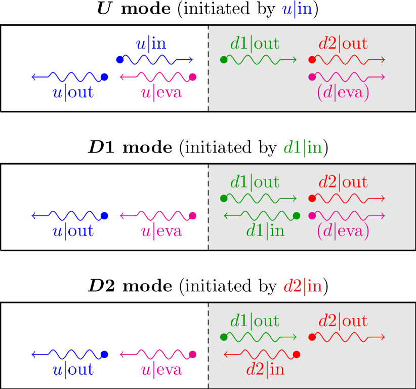
Figure 4: (Color online) The scattering modes. The color code is the same as in Fig. 3. The additional purple wiggly lines correspond to evanescent channels. For $\omega>\Omega$, the $D2$ mode disappears and the channel $d2|{\rm out}$ is replaced by $d|{\rm eva}$ in the two upper panels ($U$ and $D1$ modes). The region corresponding to the interior of the black hole is shaded as in the previous figures.

The $S$-coefficients ($S_{u,u}$, $S_{u,u}^{\rm eva}$, etc.) in Eqs. (41) are complex and do not depend on $x$ (they do depend on $\omega$ though). For each of the three scattering modes, one has four such coefficients which, once the incident channel is fixed, are determined by solving the $4\times 4$ system of linear equations (39) and (40): hence, the $S$-parameters depend on the configuration considered (flat profile, delta peak or waterfall). Physically, the square moduli $|S_{\nu^{\prime},\nu}(\omega)|^{2}$ of the $S$-matrix elements give the transmission or reflection coefficients for a $\nu$-ingoing mode of energy $\hbar\omega$ which scatters into an $\nu^{\prime}$-outgoing mode at the same energy.

Current conservation can be written in a simple matrix form provided the normalization of the real modes is defined in such a way that $J_{\ell}=\pm 1$ (as done in Secs. III.2 and III.3). Defining, for $\omega<\Omega$, the $S$-matrix as

$$S=\begin{pmatrix}S_{u,u}&S_{u,d1}&S_{u,d2}\\ S_{d1,u}&S_{d1,d1}&S_{d1,d2}\\ S_{d2,u}&S_{d2,d1}&S_{d2,d2}\end{pmatrix},$$ (42)

current conservation reads

$$S^{\dagger}\eta S=\eta=S\eta S^{\dagger},\quad\mbox{where}\quad\eta={\rm diag}(1,1,-1).$$ (43)

The coefficients such as $S_{d,u}^{\rm eva}$ are not involved in current conservation since the evanescent waves carry no current. Note that for $\omega>\Omega$, the $S$-matrix is $2\times 2$ because, the outgoing $d2$ mode – being evanescent in this case – is not involved in current conservation: one simply has the usual unitarity relation $S^{\dagger}S={\rm diag}(1,1)$. We have checked that our results for the scattering matrix indeed fulfill the $\eta$-unitarity condition (43) for $\omega<\Omega$ (and the unitarity condition for $\omega>\Omega$).

In the following we will need to determine the low-$\omega$ behavior of the components of the $S$-matrix. In the three configurations we considered, we always find that, for $\nu=u,d1,d2$, one has

$$S_{\nu,u}=f_{\nu,u}+h_{\nu,u}\varepsilon_{u}+{\cal O}(\varepsilon_{u}^{2}),$$

$$S_{\nu,d1}=\frac{f_{\nu,d1}}{\sqrt{\varepsilon_{u}}}+h_{\nu,d1}\sqrt{\varepsilon_{u}}+{\cal O}(\varepsilon_{u}^{3/2}),$$ (44)

$$S_{\nu,d2}=\frac{f_{\nu,d2}}{\sqrt{\varepsilon_{u}}}+h_{\nu,d2}\sqrt{\varepsilon_{u}}+{\cal O}(\varepsilon_{u}^{3/2}),$$

where $\varepsilon_{u}=\hbar\omega/(mc_{u}^{2})$ and the $f$’s and the $h$’s are dimensionless complex numbers. We determined them analytically in the three configurations we considered. The relevant formulae are given in Appendix A.

III.6 Quantization

The field operator $\hat{\psi}(x,t)$ associated in the Heisenberg representation to the elementary excitations on top of the background [as defined by Eq. (2)] is expanded over the scattering modes:

$$\hat{\psi}(x,t) =\mathrm{e}^{{\rm i}k_{\alpha}x}\int_{0}^{\infty}\frac{{\rm d}\omega}{\sqrt{2\pi}}\sum_{\scriptscriptstyle L\in\{U,D1\}}\Big{[}\bar{u}_{\scriptscriptstyle L}(x,\omega)\mathrm{e}^{-{\rm i}\omega t}\hat{a}_{\scriptscriptstyle L}(\omega)$$

$$\hphantom{=\mathrm{e}^{{\rm i}k_{\alpha}x}\int_{0}^{\infty}\frac{{\rm d}\omega}{\sqrt{2\pi}}\sum_{\scriptscriptstyle L\in\{U,D1\}}}+\bar{w}_{\scriptscriptstyle L}^{*}(x,\omega)\mathrm{e}^{{\rm i}\omega t}\hat{a}_{\scriptscriptstyle L}^{{\dagger}}(\omega)\Big{]}$$

$$+\mathrm{e}^{{\rm i}k_{\alpha}x}\int_{0}^{\Omega}\frac{{\rm d}\omega}{\sqrt{2\pi}}\Big{[}\bar{u}_{\scriptscriptstyle D2}(x,\omega)\mathrm{e}^{-{\rm i}\omega t}\hat{a}_{\scriptscriptstyle D2}^{{\dagger}}(\omega)$$

$$\hphantom{=\mathrm{e}^{{\rm i}k_{\alpha}x}\int_{0}^{\Omega}\frac{{\rm d}\omega}{\sqrt{2\pi}}}+\bar{w}_{\scriptscriptstyle D2}^{*}(x,\omega)\mathrm{e}^{{\rm i}\omega t}\hat{a}_{\scriptscriptstyle D2}(\omega)\Big{]},$$ (45)

where we have written explicitly the $\omega$ dependence. The $\hat{a}_{\scriptscriptstyle L}^{\dagger}(\omega)$’s create an excitation of energy $\hbar\omega$ in one of the three scattering modes ($U$, $D1$ or $D2$). They obey the following commutation relation:

$$[\hat{a}_{\scriptscriptstyle L}(\omega),\hat{a}^{\dagger}_{\scriptscriptstyle L^{\prime}}(\omega^{\prime})]=\delta_{\scriptscriptstyle L,L^{\prime}}\delta(\omega-\omega^{\prime}).$$ (46)

From expression (III.6) one sees that the $D2$ mode (which originates from the negative norm $d2|{\rm in}$ channel) is quantized in a non standard way: the role of the creation and annihilation operators is exchanged compared to the $U$ and $D1$ modes. Using the current conservation relation (43), one can show that this choice of quantization is necessary for fulfilling the appropriate Bose commutation relation of the $\hat{\psi}$ operator:

$$[\hat{\psi}(x,t),\hat{\psi}^{\dagger}(x^{\prime},t)]=\delta(x-x^{\prime}).$$ (47)

IV Radiation spectrum

The Hawking signal corresponds to emission of radiation from the interior toward the exterior of the black hole Hawking . In our specific case the energy current associated to emission of elementary excitations is (cf. Kag03 )

$$\hat{\Pi}(x,t)=-\frac{\hbar^{2}}{2m}\,\partial_{t}\hat{\Phi}^{\dagger}(x,t)\,\partial_{x}\hat{\Phi}(x,t)+{\rm h.c.},$$ (48)

where “h.c.” stands for “hermitian conjugate”. From expressions (2) and (III.6) one can write the average current $\Pi(x)=\langle\hat{\Pi}(x,t)\rangle$ under the form

$$\Pi(x)=\int_{0}^{\infty}\frac{{\rm d}\omega}{2\pi}\,\hbar\omega\,J(x,\omega),$$ (49)

where $J(x,\omega)$ [and accordingly $\Pi(x)$] can be separated in a zero temperature part $J_{0}(x,\omega)$ [$\Pi_{0}(x)$] and a “thermal part” $J_{\scriptscriptstyle T}(x,\omega)$ [$\Pi_{\scriptscriptstyle T}(x)$] with

$$J_{0}(x,\omega)=\frac{\hbar}{2m}\Big{[} -\sum_{\scriptscriptstyle L\in\{U,D1\}}\bar{w}^{*}_{\scriptscriptstyle L}(k_{\alpha}+{\rm i}\partial_{x})\bar{w}_{\scriptscriptstyle L}$$

$$+\Theta(\Omega-\omega)\bar{u}^{*}_{\scriptscriptstyle D2}(k_{\alpha}-{\rm i}\partial_{x})\bar{u}_{\scriptscriptstyle D2}\Big{]}$$

$$+{\rm c.c.}$$ (50)

and

$$J_{\scriptscriptstyle T}(x,\omega)=\sum_{\scriptscriptstyle L\in\{U,D1,D2\}}J_{\scriptscriptstyle L}(x,\omega)\,n_{\scriptscriptstyle L}(\omega),$$ (51)

where

$$J_{\scriptscriptstyle L}=\frac{\hbar}{2m}\Big{[}\bar{u}^{*}_{\scriptscriptstyle L}(k_{\alpha}-{\rm i}\partial_{x})\bar{u}_{\scriptscriptstyle L}-\bar{w}^{*}_{\scriptscriptstyle L}(k_{\alpha}+{\rm i}\partial_{x})\bar{w}_{\scriptscriptstyle L}\Big{]}+{\rm c.c.}$$ (52)

and $n_{\scriptscriptstyle L}(\omega)=\langle\hat{a}^{\dagger}_{\scriptscriptstyle L}(\omega)\hat{a}_{\scriptscriptstyle L}(\omega)\rangle$ is the occupation number of the mode $L$. Note that in expression (51) the $D2$ mode contributes only for $\omega<\Omega$. Comparing the expression (52) with (26) one sees that $J_{\scriptscriptstyle L}$ is the conserved current carried by a scattering mode $L$; it is $x$ independent for the stationary flows we consider in the present work.

Note for avoiding confusion that what we call a “zero temperature term” is the contribution to the Hawking signal that exists even when the system is at zero temperature. It will be described below (Sec. IV.2) by an effective radiation temperature $T_{\rm\scriptscriptstyle H}$ (the Hawking temperature) which is not the temperature of the BEC.

IV.1 Energy current in a black hole configuration

For large and negative $x$ (i.e., deep in the subsonic region) we show in Appendix B that formulae (41) and (IV) yield the very natural result

$$\Pi_{0}=-\int_{0}^{\Omega}\frac{{\rm d}\omega}{2\pi}\,\hbar\omega\,|S_{u,d2}(\omega)|^{2}.$$ (53)

The minus sign in this equation indicates that the energy current is directed toward $-\infty$, as clearly seen from Appendix B. If one computes the energy current for a point deep in the supersonic region (i.e., for $x$ large and positive) one gets the same result as (53), in agreement with the conservation of the energy flux in a stationary configuration. Note that the zero temperature radiation $\Pi_{0}$ vanishes in absence of black hole, as expected. In presence of a black hole, the integral gives a finite result, corresponding to a Hawking signal emitted even for $T=0$. This remark, together with the specific form of Eq. (53), shows that one needs two ingredients for having a $T=0$ Hawking radiation from a black hole: (i) a $d2|{\rm in}$ mode and (ii) a $d2\leftrightarrow u$ mode conversion, i.e., a non zero $S_{u,d2}$ coefficient. Remember that condition (i) is fulfilled only because the dispersion relation in a supersonic flow bends down at high $q$ (see Fig. 3, bottom panel), which is a consequence of the non linear behavior of the Bogoliubov dispersion relation (23). As discussed in Sec. III.1, the $d2$ incoming channel corresponds to waves whose group velocity in the frame of the condensate is larger than $V_{d}$. It is thus not surprising that these “fast” modes are involved in the Hawking radiation since they are able to overrun the flow of velocity $V_{d}$ and thus to escape the black hole. This is clearly a flaw of the BEC analogy of gravitational black holes: point (i) is certainly not fulfilled in the gravitational case since the group velocity of photons is a constant (the speed of light). As a result the number of ingoing and outgoing channels are not equal for gravitational black holes and one cannot get a stationary description of the Hawking effect: one has to take into account the dynamics of the formation of the horizon.

From Eqs. (41) and (51), the term $J_{\scriptscriptstyle T}(x,\omega)$ can be rewritten as

$$J_{\scriptscriptstyle T}(x,\omega) =\frac{2}{c_{u}\xi_{u}}\Big{[}n_{\scriptscriptstyle U}(\omega)(1-|S_{u,u}|^{2})$$

$$-n_{\scriptscriptstyle D1}(\omega)|S_{u,d1}|^{2}-n_{\scriptscriptstyle D2}(\omega)|S_{u,d2}|^{2}\Big{]}$$

$$=\frac{2}{c_{u}\xi_{u}}\Big{\{}[n_{\scriptscriptstyle U}(\omega)-n_{\scriptscriptstyle D1}(\omega)]|S_{u,d1}|^{2}$$

$$-[n_{\scriptscriptstyle U}(\omega)+n_{\scriptscriptstyle D2}(\omega)]|S_{u,d2}|^{2}\Big{\}}.$$ (54)

In absence of black hole, the $S_{u,d2}$ term in (IV.1) disappears. As a result, at thermal equilibrium, i.e., when $n_{\scriptscriptstyle U}(\omega)=n_{\scriptscriptstyle D1}(\omega)$ is a thermal Bose occupation number of the form

$$n_{\scriptscriptstyle T}(\omega)=\frac{1}{\exp\big{(}\frac{\hbar\omega}{k_{\rm\scriptscriptstyle B}T}\big{)}-1},$$ (55)

one has $J_{\scriptscriptstyle T}(x,\omega)=0$ [this is most easily seen from the last expression of $J_{\scriptscriptstyle T}$ in Eq. (IV.1)]. This is a very pleasant result demonstrating that at thermal equilibrium there is no Hawking radiation at all for any type of configuration connecting two asymptotically subsonic regions.

In the case where an acoustic horizon is present, a finite temperature configuration may be reached in the manner presented in Ref. correlations : one branches the black hole configuration adiabatically starting from a system initially uniformly subsonic at thermal equilibrium. This changes the dispersion relation in the supersonic part, but not the occupation number of the adiabatically modified modes (see the discussion in Rec09 ). In this case (IV.1) yields a finite value for the $\Pi_{\scriptscriptstyle T}$ term (because $S_{u,u}$, $n_{\scriptscriptstyle D1}$ and $n_{\scriptscriptstyle D2}$ are regular at low $\omega$).

IV.2 Hawking temperature

The zero temperature radiation $\Pi_{0}$ as given by (53) corresponds to an emission spectrum given by $|S_{u,d2}(\omega)|^{2}$. Can this be described by an effective temperature, i.e., can $|S_{u,d2}(\omega)|^{2}$ be approximated by a factor of the type $\Gamma\times n_{\scriptscriptstyle T_{\rm\scriptscriptstyle H}}(\omega)$, where $T_{\rm\scriptscriptstyle H}$ is the effective temperature of radiation? We address this question in the present subsection.

One could first argue that the addition of the “grayness factor” $\Gamma$ is an unnecessary complication of the fit of $|S_{u,d2}|^{2}$ by a thermal spectrum. Indeed, in most cases, $\Gamma$ is found to be close to 1, but this is not generally true (see the discussion below and the inset of Fig. 5) and this is the reason why we keep a certain degree of “grayness” in the present analysis.

Obviously, the identification of $|S_{u,d2}|^{2}$ with a Bose thermal factor can only be approximate because, whereas a term such as $n_{\scriptscriptstyle T_{\rm\scriptscriptstyle H}}(\omega)$ is finite for all $\omega\in\mathbb{R}^{+}$, $|S_{u,d2}|^{2}$ abruptly cancels for $\omega>\Omega$. Nonetheless one can try to find the best possible approximation by comparing the low-$\omega$ expansion of $|S_{u,d2}|^{2}$ [from Eqs. (III.5)] with $\Gamma\times n_{\scriptscriptstyle T_{\rm\scriptscriptstyle H}}(\omega)=\Gamma[k_{\rm\scriptscriptstyle B}T_{\rm\scriptscriptstyle H}/(\hbar\omega)-\frac{1}{2}+{\cal O}(\omega)]$. This immediately yields

$$\Gamma=-4\,{\rm Re}(f_{u,d2}^{*}h_{u,d2})\quad\mbox{and}\quad\frac{k_{\rm\scriptscriptstyle B}T_{\rm\scriptscriptstyle H}}{mc_{u}^{2}}=\frac{|f_{u,d2}|^{2}}{\Gamma}.$$ (56)

The analytical expressions obtained in Appendix A for $f_{u,d2}$ and $h_{u,d2}$ in the different configurations we consider yield the following estimates of the Hawking temperature:

$$\frac{k_{\rm\scriptscriptstyle B}T_{\rm\scriptscriptstyle H}}{mc_{u}^{2}}=\left\{\begin{array}[]{ll}\vspace{2mm}\displaystyle{\frac{1}{2}\frac{\mathpzc{m}_{u}^{2}}{\mathpzc{m}_{d}}\frac{(1-\mathpzc{m}_{u}^{2})(\mathpzc{m}_{d}^{2}-1)^{\frac{3}{2}}}{\mathpzc{m}_{d}^{2}-\mathpzc{m}_{u}^{2}}}&\mbox{(flat profile)},\\ \displaystyle{\frac{1}{2}\frac{(1-\mathpzc{m}_{u}^{4})^{\frac{3}{2}}}{(2+\mathpzc{m}_{u}^{2})(1+2\mathpzc{m}_{u}^{2})}}&\mbox{(waterfall)}.\end{array}\right.$$ (57)

We do not display here the formula for the delta peak configuration because it is too cumbersome. Instead we show in Fig. 5 the corresponding curve relating $T_{\rm\scriptscriptstyle H}$ to $\mathpzc{m}_{u}$ in the delta peak configuration and compare it with the results of the waterfall configuration. One first notices from the figure that $T_{\rm\scriptscriptstyle H}\to 0$ when $\mathpzc{m}_{u}\to 1$: this is expected because in this case the horizon disappears. One sees also that $T_{\rm\scriptscriptstyle H}$ remains finite in the limit $\mathpzc{m}_{u}\to 0$ in both configurations. However, this limit is singular in the sense that it corresponds to a very peculiar flow. For instance, in the waterfall configuration, the analysis of Sec. II.3 shows that the flow with $\mathpzc{m}_{u}=0$ is observed for a step with $U_{0}\to\infty$, and has downstream a zero density and an infinite velocity: the corresponding flow pattern is most probably unreachable. Moreover, one sees from the inset of Fig. 5 (and also from the analytical expression given in Appendix A) that in this case $\Gamma\to 0$ and the expected signal disappears. In the remainder of this work we rather consider a typical setting with $\mathpzc{m}_{u}=0.5$. For this value of $\mathpzc{m}_{u}$ one gets $\mathpzc{m}_{d}\simeq 1.83$ and $\Gamma\simeq 0.977$ in the delta peak configuration, $\mathpzc{m}_{d}=4$ and $\Gamma\simeq 0.980$ in the waterfall configuration.

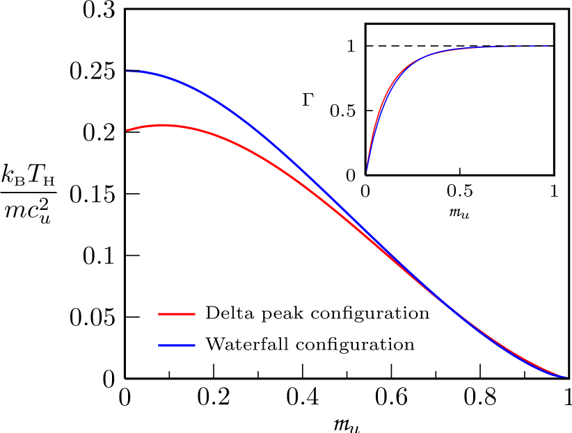
Figure 5: Normalized Hawking temperature $k_{\rm\scriptscriptstyle B}T_{\rm{\scriptscriptstyle H}}/(mc_{u}^{2})$ as a function of the upstream Mach number $\mathpzc{m}_{u}=V_{u}/c_{u}$ for the delta peak and waterfall configurations. The inset displays the grayness factor $\Gamma$ as a function of $\mathpzc{m}_{u}$ for these two configurations.

Once $T_{\rm\scriptscriptstyle H}$ is determined through the above low energy analysis, one should check, as done, e.g., in Ref. Mac09 , if the approximation of $|S_{u,d2}|^{2}$ with a thermal spectrum is accurate in the whole emission window $\omega\in[0,\Omega]$. This is done in Fig. 6 in the case of the delta peak configuration. One sees from the figure that the overall agreement is quite good. The same good agreement is obtained for the waterfall and flat profile configurations, and this legitimates the definition of a Hawking temperature in the three configurations considered in the present work. This was not a priori obvious because the concept of Hawking temperature is of semi-classical origin (see, e.g., Vol03 ) and the three configurations we consider being discontinuous, one could fear that a semi-classical analysis would fail. We see the relevance of the concept of Hawking temperature as a confirmation that the configurations considered here are typical for observing the Hawking effect. In the next section we will draw the same conclusion from a study of the density correlations.

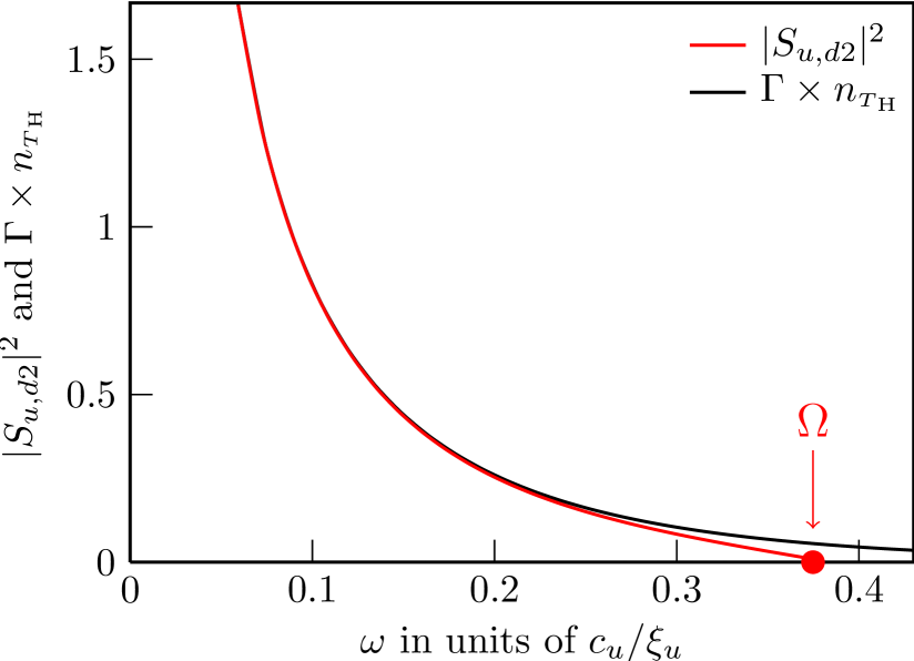
Figure 6: (Color online) Radiation spectrum in the delta peak configuration. Red curve: $|S_{u,d2}|^{2}$ as a function of the dimensionless quantity $\omega\xi_{u}/c_{u}$. Black curve: $\Gamma\times n_{\scriptscriptstyle T_{\rm\scriptscriptstyle H}}(\omega)$. The plot is drawn for $\mathpzc{m}_{u}=0.5$; in this case $k_{\rm\scriptscriptstyle B}T_{\rm\scriptscriptstyle H}/(mc_{u}^{2})\simeq 0.128$ and $\Gamma\simeq 0.977$. The difference between $|S_{u,d2}|^{2}$ and $\Gamma\times n_{\scriptscriptstyle T_{\rm\scriptscriptstyle H}}$ is maximum when $\omega=\Omega$ and is close to 0.06 in this case (for the chosen value of $\mathpzc{m}_{u}$ one has $\Omega\xi_{u}/c_{u}\simeq 0.369$).

From (57) and Fig. 5 one gets an order of magnitude $k_{\rm\scriptscriptstyle B}T_{\rm\scriptscriptstyle H}/(mc^{2}_{u})\sim 0.1$, i.e., typically $T_{\rm\scriptscriptstyle H}\sim 10$ nK. Since the temperature in typical experiments is rather of the order of the chemical potential $mc^{2}_{u}$ (i.e., around 100 nK), the Hawking radiation will be lost in the thermal noise and very difficult to identify. This is the reason why density correlations have been proposed in Ref. correlations as a tool for identifying the Hawking effect. We thus consider two-body correlations in the next section.

V Correlations

The connected two-body density matrix is defined by qu-optics

$$g^{(2)} (x_{1},x_{2})$$

$$=\langle\hat{\Phi}^{\dagger}(x_{1},t)\hat{\Phi}^{\dagger}(x_{2},t)\hat{\Phi}(x_{1},t)\hat{\Phi}(x_{2},t)\rangle$$

$$-\langle\hat{\Phi}^{\dagger}(x_{1},t)\hat{\Phi}(x_{1},t)\rangle\langle\hat{\Phi}^{\dagger}(x_{2},t)\hat{\Phi}(x_{2},t)\rangle.$$ (58)

$g^{(2)}$ is time independent because we work in a stationary configuration. In (V) the average is taken either on the ground state or over a statistical ensemble. $g^{(2)}$ is directly related to the density correlations in the system, this can be seen by rewriting Eq. (V) under the form

$$g^{(2)}(x_{1},x_{2}) =\langle\hat{n}(x_{1},t)\hat{n}(x_{2},t)\rangle-\langle\hat{n}(x_{1})\rangle\langle\hat{n}(x_{2})\rangle$$

$$-\delta(x_{1}-x_{2})\langle\hat{n}(x_{1})\rangle.$$ (59)

The last term in the right-hand side (r.h.s.) of (V) is the Poissonian fluctuation term originating from the discreteness of the particles Landau5 . Written under this form, $g^{(2)}$ is sometimes denoted as the cluster function.

For a system at thermal equilibrium in the grand canonical ensemble, one has

$$n(x) =\langle\hat{n}(x)\rangle$$

$$=\frac{1}{{\cal Z}}\,\mbox{Tr}\left\{\hat{n}(x)\exp\left[-\frac{1}{k_{\rm\scriptscriptstyle B}T}(\hat{H}-\mu\hat{N})\right]\right\},$$ (60)

where ${\cal Z}=\mbox{Tr}\{\exp[-(\hat{H}-\mu\hat{N})/(k_{\rm\scriptscriptstyle B}T)]\}$ is the partition function. Deriving expression (V) with respect to $\mu$, one gets

$$k_{\rm\scriptscriptstyle B}T\frac{\partial n(x)}{\partial\mu}=\langle\hat{n}(x)\hat{N}\rangle-\langle\hat{n}(x)\rangle\langle\hat{N}\rangle.$$ (61)

Since $\hat{N}=\int_{\mathbb{R}}{\rm d}x^{\prime}\,\hat{n}(x^{\prime})$, property (61) and expression (V) yield the following sum rule:

$$\int_{\mathbb{R}}{\rm d}x^{\prime}\,g^{(2)}(x,x^{\prime})=-n(x)+k_{\rm\scriptscriptstyle B}T\frac{\partial n(x)}{\partial\mu}.$$ (62)

For a homogeneous system, this sum rule is a standard thermodynamic result Landau5 which can be shown to be equivalent to the compressibility sum rule (whose definition is given for instance in Ref. PinesNozieres ). Formula (62) is a generalization to inhomogeneous systems; it has been used in Ref. Arm11 for witnessing quasi-condensation through a study of density fluctuations and in Ref. Zho11 to propose an universal thermometry for quantum simulations.

In the remainder of this section we concentrate on the $T=0$ case, postponing the discussion of finite temperature to a future publication. Fulfillment of the sum rule (62) is a strong test of the validity of the Bogoliubov approach used in the present work. We give in Sec. V.2 the leading order contributions to $g^{(2)}$ and explain in Appendix C how we use them in order to check that the $T=0$ version of the sum rule (62) is indeed verified for $|x|\to\infty$ (i.e., far from the horizon).

From the Bogoliubov expansion (2), one gets at leading order

$$g^{(2)}(x_{1},x_{2}) =\Phi(x_{1})\Phi^{*}(x_{2})\langle\hat{\psi}^{\dagger}(x_{1},t)\hat{\psi}(x_{2},t)\rangle$$

$$+\Phi(x_{1})\Phi(x_{2})\langle\hat{\psi}^{\dagger}(x_{1},t)\hat{\psi}^{\dagger}(x_{2},t)\rangle$$

$$+\rm{c.c.}.$$ (63)

For $i=1$ or $2$, we write $\Phi(x_{i})=\sqrt{n_{i}}\exp({\rm i}k_{i}x_{i})\phi_{i}(x_{i})$, where $n_{i}=n_{u}$ ($n_{d}$), $k_{i}=k_{u}$ ($k_{d}$) and $\phi_{i}=\phi_{u}$ ($\phi_{d}$) if $x_{i}<0$ ($x_{i}>0$). We recall that $\phi_{d}$ is defined in Eq. (6) and $\phi_{u}$ is either equal to unity (flat profile configuration) or given by Eq. (11) (delta peak and waterfall configurations). Based on the decomposition (III.6), one can show (see Ref. Rec09 ) that Eq. (V) yields

$$g^{(2)}(x_{1},x_{2})=\sqrt{n_{1}n_{2}}\int_{0}^{\infty}\frac{{\rm d}\omega}{2\pi}\,\gamma(x_{1},x_{2},\omega),$$ (64)

where $\gamma(x_{1},x_{2},\omega)$ [and accordingly $g^{(2)}(x_{1},x_{2})$] is conveniently separated in a zero temperature term $\gamma_{0}$ and a remaining term $\gamma_{\scriptscriptstyle T}$:

$$\gamma(x_{1},x_{2},\omega)=\gamma_{0}(x_{1},x_{2},\omega)+\gamma_{\scriptscriptstyle T}(x_{1},x_{2},\omega).$$ (65)

$g^{(2)}_{0}$ and $\gamma_{0}$ are the contributions evaluated from (V) and (III.6) which remain finite even in the $T=0$ case where $n_{\scriptscriptstyle L}(\omega)=\langle\hat{a}^{\dagger}_{\scriptscriptstyle L}(\omega)\hat{a}_{\scriptscriptstyle L}(\omega)\rangle=0$. One has

$$\gamma_{0}(x_{1},x_{2},\omega) =\sum_{\scriptscriptstyle L\in\{U,D1\}}\tilde{w}^{*}_{\scriptscriptstyle L}(x_{1})\tilde{r}_{\scriptscriptstyle L}(x_{2})$$

$$+\Theta(\Omega-\omega)\tilde{u}^{*}_{\scriptscriptstyle D2}(x_{1})\tilde{r}_{\scriptscriptstyle D2}(x_{2})+{\rm c.c.},$$ (66)

with

$$\tilde{u}_{\scriptscriptstyle L}(x_{i})=\phi_{i}^{*}(x_{i})\bar{u}_{\scriptscriptstyle L}(x_{i}),\quad\tilde{w}_{\scriptscriptstyle L}(x_{i})=\phi_{i}(x_{i})\bar{w}_{\scriptscriptstyle L}(x_{i}),$$ (67)

and

$$\tilde{r}_{\scriptscriptstyle L}(x_{i})=\tilde{u}_{\scriptscriptstyle L}(x_{i})+\tilde{w}_{\scriptscriptstyle L}(x_{i}).$$ (68)

The other contribution to (65) is

$$\gamma_{\scriptscriptstyle T}(x_{1},x_{2},\omega)=\!\!\!\!\sum_{\scriptscriptstyle L\in\{U,D1,D2\}}\!\!\!\!\tilde{r}_{\scriptscriptstyle L}^{*}(x_{1})\tilde{r}_{\scriptscriptstyle L}(x_{2})n_{\scriptscriptstyle L}(\omega)+{\rm c.c.},$$ (69)

where it should be understood that the $D2$ contribution is only present for $\omega<\Omega$.

We often display below the results not for $g^{(2)}$ but for the dimensionless quantity $G^{(2)}$ defined as

$$G^{(2)}(x_{1},x_{2})=\frac{g^{(2)}(x_{1},x_{2})}{n(x_{1})n(x_{2})}.$$ (70)

Also, we will compute the correlations when $x_{1}$ and $x_{2}$ are both far from the horizon. In this case, $\phi_{i}(x_{i})=\exp({\rm i}\beta_{i})$ and $G^{(2)}(x_{1},x_{2})=g^{(2)}(x_{1},x_{2})/(n_{1}n_{2})$.

V.1 No black hole

Before embarking in a general determination of $g^{(2)}$ for a black hole configuration, we recall here the result for a uniform fluid (density $n_{u}$) moving at constant subsonic velocity. One gets from the no black hole version of (V) rem1

$$\gamma_{0} (x,x^{\prime},\omega)$$

$$=\sum_{\ell\in\{u|{\rm in},u|{\rm out}\}}\tilde{w}_{\ell}^{*}(x)\tilde{r}_{\ell}(x^{\prime})+{\rm c.c.}$$ (71)

$$=\sum_{\ell\in\{u|{\rm in},u|{\rm out}\}}\frac{\frac{Q_{\ell}^{2}}{2|{E}_{\ell}|}-1}{2|V_{g}(Q_{\ell})|}\,\mathrm{e}^{{\rm i}Q_{\ell}(X^{\prime}_{u}-X_{u})}+\rm{c.c.}.$$ (72)

This yields

$$G^{(2)}_{0}(x,x^{\prime})=\frac{1}{n_{u}\xi_{u}}F\left(\frac{x-x^{\prime}}{\xi_{u}}\right),$$ (73)

where

$$F(z)=-\frac{1}{\pi z}\int_{0}^{\infty}{\rm d}t\,\frac{\sin(2\,t\,z)}{(1+t^{2})^{3/2}}.$$ (74)

This is the expected correlation in a quasi 1D condensate (see, e.g., Ref. Deu09 and references therein): $n_{u}\xi_{u}G^{(2)}_{0}(x,x^{\prime})$ is a universal function of $z=(x-x^{\prime})/\xi_{u}$. In particular, $n_{u}\xi_{u}G^{(2)}_{0}(x,x)=F(0)=-2/\pi$ Gan03 . We evaluated the fluctuations around the uniform profile numerically by means of the truncated Wigner method for the Bose field Wal94 ; Ste98 already used in correlations for studying the same observable in a black hole configuration. In Fig. 7 we compare the analytical form (73) with the results of the numerical computation along the cut displayed in the inset. The excellent agreement is a good test of the accuracy of the numerical method used in Ref. correlations .

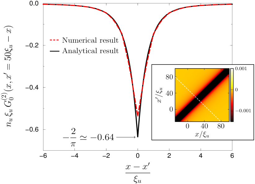
Figure 7: (Color online) $\xi_{u}n_{u}G^{(2)}_{0}(x,x^{\prime})$ computed analytically from Eq. (73) (black solid line) compared with the numerics from the truncated Wigner method (red dashed line). The small discrepancy near $x-x^{\prime}=0$ is due to numerical uncertainty and to the plotting procedure which introduces a small amount of smoothing of the raw numerical data. The inset represents a color plot of the numerical results. The white dashed line is the line $x^{\prime}=50\xi_{u}-x$ along which we compare numerical and analytical results in the main plot.

We finally note here that $\int_{\mathbb{R}}{\rm d}z\,F(z)=-1$. This yields

$$\int_{\mathbb{R}}{\rm d}x^{\prime}\,g^{(2)}_{0}(x,x^{\prime})=-n_{u},$$ (75)

which is a mere verification of the $T=0$ version of the sum rule (62) in this simple uniform setting.

The main correlation signal in the black hole configurations to be studied soon is similar to the short range anti-bunching displayed in Fig. 7. However, we will see that (i) its precise shape is affected in presence of an acoustic horizon and moreover, (ii) new long range correlations appear, which can be interpreted as emission of correlated phonons correlations .

V.2 General formulae in presence of a black hole

We now turn to the study of zero temperature density fluctuations around a sonic horizon. For simplicity, we only consider the case where $x$ and $x^{\prime}$ are far from the horizon: this makes it possible (i) to drop the evanescent contributions to (V) and (ii) to avoid treating the position dependence of the background density in the delta peak and waterfall configurations. Part of these results were already obtained in Ref. Rec09 (the ones valid when $x$ and $x^{\prime}$ are far one from the other) and here we generalize and correct some misprints misprints . We only display the most important contributions to $\gamma_{0}$ which are both the larger ones and the ones useful for fulfilling the $T=0$ version of the sum rule (62) when $x$ is far from the horizon [this version is written explicitly in Eq. (81)]. We note here that a similar approach has previously been used in Ref. Bou03 for studying phase fluctuations in a similar setting, with a description of the scattering less elaborate than the one presented in Sec. III.5.

Finally, we introduce the notations $\tilde{\cal U}_{\ell}$ and $\tilde{\cal W}_{\ell}$ defined by

$$\begin{pmatrix}\tilde{u}_{\ell}(x)\\ \tilde{w}_{\ell}(x)\end{pmatrix}=\mathrm{e}^{{\rm i}q_{\ell}x}\begin{pmatrix}\tilde{\cal U}_{\ell}(x)\\ \tilde{\cal W}_{\ell}(x)\end{pmatrix},$$ (76)

where $\tilde{u}_{\ell}(x)$ and $\tilde{w}_{\ell}(x)$ are defined in Eqs. (67). We also introduce $\tilde{\cal R}_{\ell}=\tilde{\cal U}_{\ell}+\tilde{\cal W}_{\ell}$.

V.2.1 Case $x$ and $x^{\prime}\to-\infty$

We first consider the case where $x$ and $x^{\prime}$ are both deep in the subsonic region, i.e., outside the black hole and far from the acoustic horizon. From Eq. (V), one gets in this case

$$\gamma_{0}(x,x^{\prime},\omega) =\tilde{{\cal W}}^{*}_{u|{\rm in}}\tilde{{\cal R}}_{u|{\rm in}}\mathrm{e}^{{\rm i}q_{u|{\rm in}}(x^{\prime}-x)}$$

$$+\tilde{{\cal W}}^{*}_{u|{\rm out}}\tilde{{\cal R}}_{u|{\rm out}}\mathrm{e}^{{\rm i}q_{u|{\rm out}}(x^{\prime}-x)}$$

$$+\Theta(\Omega-\omega)|S_{u,d2}|^{2}|\tilde{{\cal R}}_{u|{\rm out}}|^{2}\mathrm{e}^{{\rm i}q_{u|{\rm out}}(x^{\prime}-x)}$$

$$+\rm{c.c.}.$$ (77)

The contribution of the $S_{u,d2}$ term disappears when $\omega>\Omega$ and this is the reason for the Heaviside factor $\Theta(\Omega-\omega)$ in (V.2.1). If it were not for the $S_{u,d2}$ term, (V.2.1) would be exactly equal to (V.1), one would recover the same correlation as (73) obtained in absence of black hole and the contribution of (V.2.1) alone would be enough to verify the sum rule (75). Now the $S_{u,d2}$ term is not zero, and this means that the correlations in the vicinity of the diagonal $x=x^{\prime}$ are modified by the existence of the black hole. This is similar to the results obtained by Kravtsov and coworkers for non standard ensembles of random matrices Fra09 ; Can95 . Indeed, for fixed $x$, (V.2.1) alone is not able to fulfill the sum rule. The addition of the non local correlations (V.2.2) induced by the Hawking emission will be necessary to this end, as advocated in Ref. Fra09 .

V.2.2 Cases ($x\to-\infty$ and $x^{\prime}\to+\infty$) or ($x\to+\infty$ and $x^{\prime}\to-\infty$)

In the case where $x$ is deep in the upstream region and $x^{\prime}$ deep in the downstream one, we get

$$\gamma_{0}(x,x^{\prime},\omega) =\Theta(\Omega-\omega)S^{*}_{u,d2}S_{d1,d2}\times$$

$$\hphantom{\textrm{}+\textrm{}}\tilde{\cal R}^{*}_{u|\rm{out}}\tilde{\cal R}_{d1|\rm{out}}\mathrm{e}^{{\rm i}(q_{d1|\rm{out}}x^{\prime}-q_{u|\rm{out}}x)}$$

$$+\Theta(\Omega-\omega)S^{*}_{u,d2}S_{d2,d2}\times$$

$$\hphantom{\textrm{}+\textrm{}}\tilde{\cal R}^{*}_{u|\rm{out}}\tilde{\cal R}_{d2|\rm{out}}\mathrm{e}^{{\rm i}(q_{d2|\rm{out}}x^{\prime}-q_{u|\rm{out}}x)}$$

$$+{\rm c.c.}.$$ (78)

If instead $x$ is deep in the downstream supersonic region and $x^{\prime}$ deep in the upstream subsonic region, it suffices to exchange the roles of $x$ and $x^{\prime}$ in the above formula.

V.2.3 Case $x$ and $x^{\prime}\to+\infty$

This is the case where $x$ and $x^{\prime}$ are both deep in the downstream region (i.e., deep inside the black hole). The leading order contribution to $g^{(2)}_{0}$ can be separated in a diagonal part which depends only on $x-x^{\prime}$ and a non diagonal part. The diagonal part reads

$$\gamma_{0}^{\rm diag}(x,x^{\prime},\omega) =\tilde{{\cal W}}^{*}_{d1|{\rm in}}\tilde{{\cal R}}_{d1|{\rm in}}\mathrm{e}^{{\rm i}q_{d1|{\rm in}}(x^{\prime}-x)}$$

$$+\tilde{{\cal W}}^{*}_{d1|{\rm out}}\tilde{{\cal R}}_{d1|{\rm out}}\mathrm{e}^{{\rm i}q_{d1|{\rm out}}(x^{\prime}-x)}$$

$$+\Theta(\Omega-\omega)\tilde{{\cal U}}^{*}_{d2|{\rm in}}\tilde{{\cal R}}_{d2|{\rm in}}\mathrm{e}^{{\rm i}q_{d2|{\rm in}}(x^{\prime}-x)}$$

$$+\Theta(\Omega-\omega)\tilde{{\cal U}}^{*}_{d2|{\rm out}}\tilde{{\cal R}}_{d2|{\rm out}}\mathrm{e}^{{\rm i}q_{d2|{\rm out}}(x^{\prime}-x)}$$

$$+\Theta(\Omega-\omega)|S_{d1,d2}|^{2}|\tilde{{\cal R}}_{d1|{\rm out}}|^{2}\mathrm{e}^{{\rm i}q_{d1|{\rm out}}(x^{\prime}-x)}$$

$$+\Theta(\Omega-\omega)(|S_{d2,u}|^{2}+|S_{d2,d1}|^{2})\times$$

$$\hphantom{\textrm{}+\textrm{}}|\tilde{{\cal R}}_{d2|{\rm out}}|^{2}\mathrm{e}^{{\rm i}q_{d2|{\rm out}}(x^{\prime}-x)}$$

$$+\rm{c.c.}.$$ (79)

In absence of black hole, the terms involving coefficients of the $S$-matrix disappear in (V.2.3) and this gives, after integration over $\omega\in\mathbb{R}^{+}$, the usual quasi-condensate correlation signal: $g_{0}^{(2)}(x,x^{\prime})=n_{d}F[(x-x^{\prime})/\xi_{d}]/\xi_{d}$.

The non diagonal part is only present if a horizon exists and only contributes for $\omega<\Omega$; it reads

$$\gamma_{0}^{\textrm{non-diag}}(x,x^{\prime},\omega) =\Theta(\Omega-\omega)S^{*}_{d1,d2}S_{d2,d2}\times$$

$$\hphantom{\textrm{}+\textrm{}}\tilde{\cal R}^{*}_{d1|\rm{out}}\tilde{\cal R}_{d2|\rm{out}}\mathrm{e}^{{\rm i}(q_{d2|{\rm out}}x^{\prime}-q_{d1|{\rm out}}x)}$$

$$+(x\longleftrightarrow x^{\prime})+\rm{c.c.}.$$ (80)

V.3 Results for the three configurations

Formulae (V.2.1), (V.2.2), (V.2.3) and (V.2.3) allow us to determine $g^{(2)}_{0}(x,x^{\prime})$ through Eq. (64). We performed the corresponding integration over $\omega\in\mathbb{R}^{+}$ numerically. The results are shown in Fig. 8 for the delta peak configuration and in Fig. 9 for the waterfall configuration. In each of these figures we only display the correlations for $|x|$ and $|x^{\prime}|$ larger than a few healing lengths, because we use formulae which are exact only in the limit $|x|$ and $|x^{\prime}|\to\infty$.

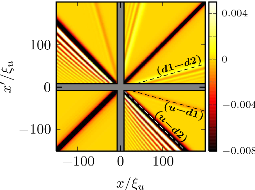
Figure 8: (Color online) 2D plot of the numerical result for the quantity $\xi_{u}n_{u}G^{(2)}_{0}(x,x^{\prime})$ in the case of a delta peak configuration with $\mathpzc{m}_{u}=0.5$. The shaded area near the axis corresponds to the zone $|x|$ or $|x^{\prime}|<10\xi_{u}$. $G^{(2)}_{0}$ is only displayed for $|x|$ and $|x^{\prime}|>10\xi_{u}$, i.e., in the asymptotic region where expressions (V.2.1), (V.2.2), (V.2.3) and (V.2.3) are valid. The dashed straight lines correspond to the correlation lines where a heuristic interpretation of the Hawking signal leads to expect the largest signal (see the text).

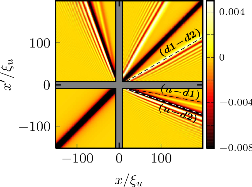
Figure 9: (Color online) Same as Fig. 8 for a waterfall configuration with $\mathpzc{m}_{u}=0.5$.

In each plot, we also display the lines where the heuristic interpretation of the Hawking effect presented in the introduction (see also Ref. correlations ) leads to locate the more pronounced correlation signal: if correlated Hawking phonons are emitted along the $u|{\rm out}$, $d1|{\rm out}$ and $d2|{\rm out}$ channels, at time $t$ after their emission, these phonons are respectively located at $x_{u|{\rm out}}=(V_{u}-c_{u})t<0$, $x_{d1|{\rm out}}=(V_{d}+c_{d})t>0$ and $x_{d2|{\rm out}}=(V_{d}-c_{d})t>0$ rem2 . This induces a correlation signal along lines of slopes: $(V_{u}-c_{u})/(V_{d}+c_{d})$ (resulting from $u-d1$ correlations), $(V_{u}-c_{u})/(V_{d}-c_{d})$ ($u-d2$ correlations) and $(V_{d}-c_{d})/(V_{d}+c_{d})$ ($d1-d2$ correlations). Of course the lines with inverse slopes are also present (they correspond to the exchange $x\leftrightarrow x^{\prime}$). Indeed, the main features of the computed $g^{(2)}_{0}$ perfectly match this interpretation of the Hawking effect.

These results are very similar to the ones obtained numerically for the flat profile configuration (already displayed in Refs. correlations ; Rec09 ). This legitimizes the use of density correlations as a tool for identifying Hawking radiation also in the realistic delta peak and waterfall configurations.

For each plot the dominant signal is the anti-bunching along the diagonal ($x=x^{\prime}$). This corresponds to the typical local density correlation in a quasi-condensate (cf. Fig. 7). However, this signal is modified compared to the one observed in a uniform system (see, e.g., the discussion in Sec. V.2.1). This modification is connected to non local features which are necessary to verify the sum rule

$$\int_{\mathbb{R}}{\rm d}x^{\prime}\,g^{(2)}_{0}(x,x^{\prime})=\left\{\begin{array}[]{lcl}-n_{u}&\mbox{when}&x\to-\infty,\\ -n_{d}&\mbox{when}&x\to+\infty,\end{array}\right.$$ (81)

which is the $T=0$ version of the sum rule (62) valid when $x$ is far from the horizon. We checked this sum rule analytically in Appendix C on the basis of our Bogoliubov description of the quantum fluctuations and of the results of Secs. V.2.1, V.2.2 and V.2.3.

By comparing Figs. 8 and 9 with the inset of Fig. 7, one can reverse the argument of Ref. Fra09 and argue that (i) in presence of an acoustic horizon, the main new features of $g^{(2)}_{0}$ are the non local density correlations which are simply understood as resulting from the emission of correlated phonons and (ii) because of the sum rule (81), these long range correlations have to be associated to modifications of the short range behavior of $g^{(2)}_{0}$. However, these short range modifications are not of great experimental relevance because they would be efficiently blurred by finite temperature effects. The non local aspects instead are good signatures of the Hawking effect because they are easily distinguished from the thermal noise (being even reinforced at finite $T$ as demonstrated in Ref. Rec09 ).

VI Conclusion and discussion

In the present work we have introduced new and realistic acoustic analogs of black holes and have analyzed the associated Hawking radiation. We restricted ourself to simple configurations (flat profile, delta peak, waterfall) but our approach is easily applied to more complicated cases. For instance, in a wave guide with a constriction, one is in a mixed situation where there is an external potential step (as in the waterfall configuration) whereas the non linear parameter is position-dependent (as in the flat profile configuration) Leb03 . This case is interesting since it may be possible to realize it experimentally, but the analytical treatment is straightforward and we do not consider it here because this would bring no new insight on our theoretical method. One could also consider smooth potentials, and the eigen-modes (defined in Sec. III) should then be determined numerically, but the theoretical framework presented here remains of course valid in this situation. We note also that the present approach can be adapted to treat the creation of a black hole horizon in a Fermi gas as suggested in Ref. Gio05 .

The description of the system in terms of a $S$-matrix allows for a simple description of the radiation spectrum and a clear identification of the characteristics of the system. In particular, we showed that Hawking radiation is absent for a “no black hole configuration” corresponding to a flow connecting two subsonic asymptotic regions. The spectrum of Hawking radiation has been computed in the case of a black hole connecting an upstream subsonic region to a downstream supersonic one, and the concept of Hawking temperature has been discussed quantitatively.

The main focus has been put on non local density correlations. We verified that their interpretation in terms of emission of correlated phonons previously introduced in a model configuration correlations ; Rec09 also holds in realistic settings. By studying a sum rule verified by the two-body density matrix, we showed that the Bogoliubov description of the quantum fluctuations around the stationary ground state of the system also provides an accurate description of the short range density correlations.

In this work we introduced new acoustic black hole configurations motivated by their possible experimental realization and proposed – following Ref. correlations – non local density correlations as practical signatures of Hawking radiation. It is thus important to discuss if the proposed signal is large enough for being detected experimentally. From Figs. 8 and 9, one sees that the prominent Hawking signal corresponds to $u-d2$ correlations. For each figure this corresponds to a line of negative correlation where the largest value of $\xi_{u}n_{u}G^{(2)}_{0}$ is between $-0.01$ and $-0.02$. In present-day experiments it is possible to measure density fluctuations around a mean density $n_{u}$ of order 10 $\mu$m^-1 in a setting where the healing length $\xi_{u}$ is around a few $\mu$m (see, e.g., Ref. Arm11 ). It is thus realistic to hope to reach a configuration where $|G^{(2)}_{0}|_{\rm max}\simeq 5\times 10^{-3}$, and for detecting a signal of this intensity a precision of around $10^{-4}$ is required on the determination of $G^{(2)}$. Noticing that $G^{(2)}$ is the quadratic relative density fluctuations, detecting this signal would correspond to measuring density fluctuations with a precision of order of 1 %, which seems within reach of present-day experimental techniques.

Appendix A Low energy behavior of the scattering matrix

In this appendix we display the analytical results for the low-$\omega$ behavior of combinations of the elements of the $S$-matrix relevant for computations of the Hawking temperature and for the fulfillment of the sum rule (81). We only give results for the flat profile and waterfall configurations because those concerning the delta peak configuration are too long. Indeed, for the delta peak configuration, a numerical determination of the coefficients of the $S$-matrix (which simply amounts to invert a $4\times 4$ matrix) is more convenient than the analytical approach. We checked that both agreed to an extremely good accuracy.

A.1 Flat profile configuration

In this case, the scattering coefficients depend of the two Mach numbers $\mathpzc{m}_{u}$ and $\mathpzc{m}_{d}$. The coefficients $f$ and $h$ defined in Eqs. (III.5) verify the following relations

$$|f_{u,d2}|^{2}=2\frac{\mathpzc{m}_{u}}{\mathpzc{m}_{d}}\frac{\mathpzc{m}_{u}^{2}}{\mathpzc{m}_{d}^{2}-\mathpzc{m}_{u}^{2}}\frac{1-\mathpzc{m}_{u}}{1+\mathpzc{m}_{u}}(\mathpzc{m}_{d}^{2}-1)^{\frac{3}{2}},$$ (82)

$$|f_{d1,d2}|^{2}=\frac{1}{2}\left(\frac{\mathpzc{m}_{u}}{\mathpzc{m}_{d}}\right)^{2}\frac{\mathpzc{m}_{d}-\mathpzc{m}_{u}}{\mathpzc{m}_{d}+\mathpzc{m}_{u}}\frac{1-\mathpzc{m}_{u}}{1+\mathpzc{m}_{u}}(\mathpzc{m}_{d}^{2}-1)^{\frac{3}{2}},$$ (83)

$$|f_{d2,d2}|^{2}=\frac{1}{2}\left(\frac{\mathpzc{m}_{u}}{\mathpzc{m}_{d}}\right)^{2}\frac{\mathpzc{m}_{d}+\mathpzc{m}_{u}}{\mathpzc{m}_{d}-\mathpzc{m}_{u}}\frac{1-\mathpzc{m}_{u}}{1+\mathpzc{m}_{u}}(\mathpzc{m}_{d}^{2}-1)^{\frac{3}{2}},$$ (84)

$$f_{u,d2}^{*}f_{d1,d2}=\left(\frac{\mathpzc{m}_{u}}{\mathpzc{m}_{d}}\right)^{\frac{3}{2}}\frac{\mathpzc{m}_{u}}{\mathpzc{m}_{d}+\mathpzc{m}_{u}}\frac{1-\mathpzc{m}_{u}}{1+\mathpzc{m}_{u}}(\mathpzc{m}_{d}^{2}-1)^{\frac{3}{2}},$$ (85)

$$f_{u,d2}^{*}f_{d2,d2}=-\left(\frac{\mathpzc{m}_{u}}{\mathpzc{m}_{d}}\right)^{\frac{3}{2}}\frac{\mathpzc{m}_{u}}{\mathpzc{m}_{d}-\mathpzc{m}_{u}}\frac{1-\mathpzc{m}_{u}}{1+\mathpzc{m}_{u}}(\mathpzc{m}_{d}^{2}-1)^{\frac{3}{2}},$$ (86)

$$f_{d1,d2}^{*}f_{d2,d2}=-\frac{1}{2}\left(\frac{\mathpzc{m}_{u}}{\mathpzc{m}_{d}}\right)^{2}\frac{1-\mathpzc{m}_{u}}{1+\mathpzc{m}_{u}}(\mathpzc{m}_{d}^{2}-1)^{\frac{3}{2}},$$ (87)

$$\mbox{Re}(f^{*}_{u,d2}h_{u,d2})=-\frac{\mathpzc{m}_{u}}{(1+\mathpzc{m}_{u})^{2}}.$$ (88)

A.2 Waterfall configuration

In the case of the waterfall configuration, the elements of the $S$-matrix depend on a unique parameter; we chose to express them as functions of the Mach number $\mathpzc{m}_{u}$.

$$|f_{u,d2}|^{2}=2\frac{\mathpzc{m}_{u}(1-\mathpzc{m}_{u})^{\frac{3}{2}}(1+\mathpzc{m}_{u}^{2})^{\frac{3}{2}}}{(1+\mathpzc{m}_{u})^{\frac{1}{2}}(1+\mathpzc{m}_{u}+\mathpzc{m}_{u}^{2})^{2}},$$ (89)

$$|f_{d1,d2}|^{2}=\frac{1}{2}\frac{(1-\mathpzc{m}_{u})^{\frac{7}{2}}(1+\mathpzc{m}_{u}^{2})^{\frac{3}{2}}}{(1+\mathpzc{m}_{u})^{\frac{1}{2}}(1+\mathpzc{m}_{u}+\mathpzc{m}_{u}^{2})^{2}},$$ (90)

$$|f_{d2,d2}|^{2}=\frac{1}{2}\frac{(1-\mathpzc{m}_{u}^{4})^{\frac{3}{2}}}{(1+\mathpzc{m}_{u}+\mathpzc{m}_{u}^{2})^{2}},$$ (91)

$$f_{u,d2}^{*}f_{d1,d2}=-\frac{\mathpzc{m}_{u}^{\frac{1}{2}}(1-\mathpzc{m}_{u})^{\frac{5}{2}}(1+\mathpzc{m}_{u}^{2})^{\frac{3}{2}}}{(1+\mathpzc{m}_{u})^{\frac{1}{2}}(1+\mathpzc{m}_{u}+\mathpzc{m}_{u}^{2})^{2}},$$ (92)

$$f_{u,d2}^{*}f_{d2,d2}=-\frac{\mathpzc{m}_{u}^{\frac{1}{2}}(1+\mathpzc{m}_{u})^{\frac{1}{2}}(1-\mathpzc{m}_{u})^{\frac{3}{2}}(1+\mathpzc{m}_{u}^{2})^{\frac{3}{2}}}{(1+\mathpzc{m}_{u}+\mathpzc{m}_{u}^{2})^{2}},$$ (93)

$$f_{d1,d2}^{*}f_{d2,d2}=\frac{1}{2}\frac{(1+\mathpzc{m}_{u})^{\frac{1}{2}}(1-\mathpzc{m}_{u})^{\frac{5}{2}}(1+\mathpzc{m}_{u}^{2})^{\frac{3}{2}}}{(1+\mathpzc{m}_{u}+\mathpzc{m}_{u}^{2})^{2}},$$ (94)

$$\mbox{Re}(f_{u,d2}^{*}h_{u,d2})=-\frac{\mathpzc{m}_{u}(2+\mathpzc{m}_{u}^{2})(1+2\mathpzc{m}_{u}^{2})}{(1+\mathpzc{m}_{u})^{2}(1+\mathpzc{m}_{u}+\mathpzc{m}_{u}^{2})^{2}}.$$ (95)

Appendix B Computation of the energy current

In this appendix we briefly indicate how formula (53) is obtained from Eqs. (49) and (IV). For a point $x$ deep in the subsonic region, using the $\eta$-unitarity (43) of the $S$-matrix, one can write the relevant contributions to $J_{0}(x,\omega)$ in (IV) under the form

$$J_{0}(x,\omega) =(q_{u|{\rm in}}-k_{u})|\tilde{{\cal W}}_{u|{\rm in}}|^{2}+(q_{u|{\rm out}}-k_{u})|\tilde{{\cal W}}_{u|{\rm out}}|^{2}$$

$$+|S_{u,d2}|^{2}\Big{[}(q_{u|{\rm out}}+k_{u})|\tilde{{\cal U}}_{u|{\rm out}}|^{2}$$

$$\hphantom{+|S_{u,d2}|^{2}\Big{[}}+(q_{u|{\rm out}}-k_{u})|\tilde{{\cal W}}_{u|{\rm out}}|^{2}\Big{]}.$$ (96)

A simple but lengthly computation shows that the contributions to $\Pi_{0}$ of the two first terms of the r.h.s. of (B) cancel after integration over $\omega$. This is very satisfactory because this shows that there is no Hawking radiation when $S_{u,d2}=0$, i.e., in absence of black hole.

Using Eq. (III.1) the remaining can be written as $|S_{u,d2}|^{2}J_{u|{\rm out}}/\xi_{u}c_{u}$, and since $\hbar/(mc_{u}\xi_{u})=1$ this directly yields Eq. (53). The minus sign in this formula comes from the fact that $J_{u|{\rm out}}=-1$ and corresponds to the direction of propagation of the energy in the $u|{\rm out}$ mode.

Appendix C Verification of the sum rule (62)

In this appendix we check that the Bogoliubov approach based on expansion (III.6) indeed makes it possible to verify Eq. (81) which is the $T=0$ version of the sum rule (62) when $x$ is far from the sonic horizon, either upstream or downstream.

We start here by a technical remark. For fixed $x$, the contributions to $\gamma_{0}(x,x^{\prime},\omega)$ displayed in Secs. V.2.1, V.2.2 and V.2.3 are only noticeable for $x^{\prime}\ll-\xi_{u}$ or $x^{\prime}\gg\xi_{d}$. As a result, the analytical forms displayed in these sections can be extended for all $x^{\prime}\in\mathbb{R}$ without introducing noticeable errors in the computation of the integral of $\gamma_{0}(x,x^{\prime},\omega)$ over $x^{\prime}$. Then, the integration of $\gamma_{0}(x,x^{\prime},\omega)$ over $x^{\prime}$ just amounts to evaluating the following integral:

$$\int_{\mathbb{R}}{\rm d}x^{\prime}\,\mathrm{e}^{{\rm i}q_{\ell}(\omega)x^{\prime}}=$$ (97)

$$\left\{\begin{array}[]{ccl}0&\mbox{if}&\ell\in\{d1|{\rm in},d2|{\rm in}\},\\ |V_{g}(Q_{\ell}(0))|\delta(\omega)&\mbox{if}&\ell\in\{u|{\rm in},u|{\rm out},d1|{\rm out},d2|{\rm out}\}.\end{array}\right.$$ (100)

In (97) we used the fact that $q_{d1|{\rm in}}$ and $q_{d2|{\rm in}}$ never cancel, whereas the other $q_{\ell}$’s do for $\omega=0$ (see Fig. 3). Using this prescription, for $x$ large and negative, one gets from Eq. (V.2.1)

$$\int_{\mathbb{R}^{-}}{\rm d}x^{\prime}\,n_{u}\int_{0}^{\infty}\frac{{\rm d}\omega}{2\pi}\,\gamma_{0}(x,x^{\prime},\omega)$$

$$=-n_{u}+\frac{n_{u}}{2}\frac{|f_{u,d2}|^{2}}{1-\mathpzc{m}_{u}},$$ (101)

and from Eq. (V.2.2)

$$\int_{\mathbb{R}^{+}}{\rm d}x^{\prime}\,\sqrt{n_{u}n_{d}}\int_{0}^{\infty}\frac{{\rm d}\omega}{2\pi}\,\gamma_{0}(x,x^{\prime},\omega)$$

$$=\frac{n_{u}}{2}\sqrt{\frac{c_{u}}{c_{d}}\frac{n_{d}}{n_{u}}}\,\mbox{Re}\left[\frac{f_{u,d2}^{*}}{1-\mathpzc{m}_{u}}(f_{d1,d2}+f_{d2,d2})\right].$$ (102)

Altogether this yields

$$\lim_{x\to-\infty}\int_{\mathbb{R}}{\rm d}x^{\prime}\,g_{0}(x,x^{\prime})=-n_{u}$$

$$+\frac{n_{u}}{2}\sqrt{\frac{c_{u}}{c_{d}}\frac{n_{d}}{n_{u}}}\,\mbox{Re}\left(\frac{f_{u,d2}^{*}}{1-\mathpzc{m}_{u}}{\cal F}\right),$$ (103)

where

$${\cal F}=f_{u,d2}\sqrt{\frac{c_{d}}{c_{u}}\frac{n_{u}}{n_{d}}}+f_{d1,d2}+f_{d2,d2}.$$ (104)

Similarly one gets [from Eqs. (V.2.2), (V.2.3) and (V.2.3)]

$$\lim_{x\to+\infty}\int_{\mathbb{R}}{\rm d}x^{\prime}\,g^{(2)}_{0}(x,x^{\prime})=-n_{d}$$

$$+\frac{n_{d}}{2}\left(\frac{c_{u}}{c_{d}}\right)^{2}\mbox{Re}\left[\left(\frac{f_{d1,d2}^{*}}{\mathpzc{m}_{d}+1}+\frac{f_{d2,d2}^{*}}{\mathpzc{m}_{d}-1}\right){\cal F}\right].$$ (105)

Using the analytical expressions for the combinations of coefficients $f_{u,d2}$, $f_{d1,d2}$ and $f_{d2,d2}$ displayed in Appendix A, one can easily verify that the second terms of the r.h.s. of Eqs. (C) and (C) cancel. This is due to the fact that ${\cal F}$ is identically null in the flat profile and waterfall configurations (this is more tedious to check but we confirmed it analytically). The same holds for the delta peak configuration. This shows that the sum rule (81) is fulfilled in these three cases. This is a strong confirmation of both the validity of the Bogoliubov approach and of the exactness of our analytical results.

References

- (1) W. G. Unruh, Phys. Rev. Lett. 46, 1351 (1981).
- (2) L. J. Garay, J. R. Anglin, J. I. Cirac and P. Zoller, Phys. Rev. Lett. 85, 4643 (2000); C. Barceló, S. Liberati and M. Visser, Int. J. Mod. Phys. A 18, 3735 (2003); C. Barceló, S. Liberati and M. Visser, Phys. Rev. A 68, 053613 (2003); S. Giovanazzi, C. Farrell, T. Kiss and U. Leonhardt, Phys. Rev. A 70, 063602 (2004); C. Barceló, S. Liberati and M. Visser, Living Rev. Relativity 8, 12 (2005); R. Schützhold, Phys. Rev. Lett. 97, 190405 (2006); S. Wüster and C. M. Savage, Phys. Rev. A 76, 013608 (2007); Y. Kurita and T. Morinari, Phys. Rev. A 76, 053603 (2007).
- (3) O. Lahav, A. Itah, A. Blumkin, C. Gordon, S. Rinott, A. Zayats and J. Steinhauer, Phys. Rev. Lett. 105, 240401 (2010).
- (4) T. G. Philbin et al., Science 319, 1367 (2008); F. Belgiorno et al., Phys. Rev. Lett. 105, 203901 (2010); I. Fouxon, O. V. Farberovich, S. Bar-Ad and V. Fleurov, EuroPhys. Lett. 92 14002 (2010); M. Elazar, V. Fleurov and S. Barad, Nonlinear Optics: Materials, Fundamentals and Applications, OSA Technical Digest (CD) (Optical Society of America, 2011), paper NTuE6.
- (5) G. Rousseaux et al., New J. Phys. 12, 095018 (2010); S. Weinfurtner, E. W. Tedford, M. C. J. Penrice, W. G. Unruh and G. A. Lawrence, Phys. Rev. Lett. 106, 021302 (2011).
- (6) R. Balbinot, A. Fabbri, S. Fagnocchi, A. Recati and I. Carusotto, Phys. Rev. A 78, 021603 (2008); I. Carusotto, S. Fagnocchi, A. Recati, R. Balbinot and A. Fabbri, New J. Phys. 10, 103001 (2008).
- (7) S. W. Hawking, Nature 248, 30 (1974); Comm. Math. Phys. 43, 199 (1975).
- (8) M. K. Parikh, Int. J. Mod. Phys. D 13, 2351 (2004).
- (9) A. Recati, N. Pavloff and I. Carusotto, Phys. Rev. A 80, 043603 (2009).
- (10) U. Leonhardt, T. Kiss and P. Öhberg, J. Opt. B: Quantum Semiclass. Opt. 5, S42 (2003); Phys. Rev. A 67, 033602 (2003).
- (11) J. Macher and R. Parentani, Phys. Rev. A 80, 043601 (2009); Phys. Rev. D 79, 124008 (2009).
- (12) F. Franchini and V. E. Kravtsov, Phys. Rev. Lett. 103, 166401 (2009).
- (13) C. M. Canali and V. E. Kravtsov, Phys. Rev. E 51, 5185(R) (1995).
- (14) C. Menotti and S. Stringari, Phys. Rev. A 66, 043610 (2002).
- (15) M. Olshanii, Phys. Rev. Lett. 81, 938 (1998).
- (16) P. Leboeuf and N. Pavloff, Phys. Rev. A 64, 033602 (2001); N. Pavloff, Phys. Rev. A 66, 013610 (2002).
- (17) I. Zapata, M. Albert, R. Parentani and F. Sols, New. J. Phys. 13, 063048 (2011).
- (18) A. Kamchatnov and N. Pavloff, arXiv:1111.5134.
- (19) P. Leboeuf, N. Pavloff and S. Sinha, Phys. Rev. A 68, 063608 (2003).
- (20) C. Barcelo, L. J. Garay and G. Jannes, Phys. Rev. D 82, 044042 (2010).
- (21) J.P. Blaizot, G. Ripka, Quantum Theory of Finite Systems, (MIT Press, 1986).
- (22) A. L. Fetter, in Bose-Einstein condensation in atomic gases, Proceedings of the 1998 “Enrico Fermi” International School, course CXL, edited by M. Inguscio, S. Stringari and C. E. Wieman, p. 201 (IOS Press, Amsterdam, 1999).
- (23) F. Dalfovo, A. Fraccheti, A. Lastri, L. Pitaevskii and S. Stringari, J. Low Temp. Phys. 104, 367 (1996).
- (24) Remember that the value of depends on the configuration considered, for instance in the flat profile configuration.
- (25) N. Bilas and N. Pavloff, Phys. Rev. A 72, 033618 (2005).
- (26) Yu. Kagan, D. L. Kovrizhin and L. A. Maksimov, Phys. Rev. Lett. 90, 130402 (2003).
- (27) G. E. Volovik, The Universe in a Helium Droplet, The International Series of Monographs on Physics vol. 117 (Oxford University Press, New-York, 2009).
- (28) For our study it is more appropriate to withdraw the disconnected terms in (V) and we thus do not follow the usual quantum optics notation.
- (29) L. D. Landau and E. M. Lifshitz, Statistical Physics, Course of Theoretical Physics, Volume 5 (Butterworth-Heinemann, 1980).
- (30) D. Pines and P. Nozières, The Theory of Quantum Liquids, (Benjamin, New-York, 1966).
- (31) J. Armijo, T. Jacqmin, K. Kheruntsyan and I. Bouchoule, Phys. Rev. A 83, 021605(R) (2011).
- (32) Qi Zhou and Tin-Lun Ho, Phys. Rev. Lett. 106, 225301 (2011).
- (33) I. Bouchoule and K. Mølmer, Phys. Rev. A 67, 011603(R) (2003).
- (34) In this case one does not have the complicated scattering modes (41) relevant for a black hole configuration. One just has two free modes – propagating either to the left or to the right – which are exactly identical to the modes and identified in Sec. III.1, and the -matrix is the identity.
- (35) P. Deuar et al., Phys. Rev. A 79, 043619 (2009).
- (36) D. M. Gangardt and G. V. Shlyapnikov, Phys. Rev. Lett. 90, 010401 (2003).
- (37) D. F. Walls and G. J. Milburn, Quantum Optics (Springer, Berlin, 1994).
- (38) M. J. Steel et al., Phys. Rev. A 58, 4824 (1998).
- (39) In Eqs. (27), (29), (33), (36), (39) and (40) of Ref. Rec09 the prefactor should be instead of . Also the argument of the exponential in formulae (27) and (33) has the wrong sign.
- (40) This is obtained assuming linear dispersion relations along each branch of the dispersion relation, which is a long wavelength approximation.
- (41) S. Giovanazzi, Phys. Rev. Lett. 94, 061302 (2005); J. Phys. B: At. Mol. Opt. Phys. 39, S109 (2006).