A Revised Effective Temperature Scale for the Kepler Input Catalog

Abstract

We present a catalog of revised effective temperatures for stars observed in long-cadence mode in the Kepler Input Catalog (KIC). We use SDSS $griz$ filters tied to the fundamental temperature scale. Polynomials for $griz$ color-temperature relations are presented, along with correction terms for surface gravity effects, metallicity, and statistical corrections for binary companions or blending. We compare our temperature scale to the published infrared flux method (IRFM) scale for $V_{T}JK_{s}$ in both open clusters and the Kepler fields. We find good agreement overall, with some deviations between $(J\,-\,K_{s})$-based temperatures from the IRFM and both SDSS filter and other diagnostic IRFM color-temperature relationships above $6000$ K. For field dwarfs we find a mean shift towards hotter temperatures relative to the KIC, of order $215$ K, in the regime where the IRFM scale is well-defined ($4000$ K to $6500$ K). This change is of comparable magnitude in both color systems and in spectroscopy for stars with $T_{\rm eff}$ below $6000$ K. Systematic differences between temperature estimators appear for hotter stars, and we define corrections to put the SDSS temperatures on the IRFM scale for them. When the theoretical dependence on gravity is accounted for we find a similar temperature scale offset between the fundamental and KIC scales for giants. We demonstrate that statistical corrections to color-based temperatures from binaries are significant. Typical errors, mostly from uncertainties in extinction, are of order $100$ K. Implications for other applications of the KIC are discussed.

1. Introduction

One of the most powerful applications of stellar multi-color photometry is the ability to precisely infer crucial global properties. Photometric techniques are especially efficient for characterizing large samples and providing basic constraints for more detailed spectroscopic studies. Modern surveys frequently used filters designed for the Sloan Digital Sky Survey (SDSS; Aihara et al., 2011), however, while traditional correlations between color and effective temperature ($T_{\rm eff}$), metallicity ([Fe/H]), and surface gravity ($\log{g}$) have employed other filter sets, typically on the Johnson-Cousins system. In An et al. (2009a, hereafter A09) we used SDSS photometry of a solar-metallicity cluster M67 (An et al., 2008) to define a photometric $ugriz$–$T_{\rm eff}$ relation, and checked the metallicity scale using star clusters over a wide range of metallicity. This scale was applied to the Virgo overdensity in the halo by An et al. (2009b). The approach used is similar in spirit to earlier work in the Johnson-Cousins filter system (Pinsonneault et al., 2003, 2004; An et al., 2007a, b); the latter effort used the color-temperature relationships of Lejeune et al. (1997, 1998) with empirical corrections based on cluster studies.

A revised color-temperature-metallicity relationship for late-type stars has recently been published by Casagrande et al. (2010, hereafter C10); it is based on the infrared flux method (IRFM). There are a number of advantages of this approach, as discussed in C10, but there is a lack of native SDSS data in the stars used to define the calibration itself. Fortunately, the color-temperature relationships in C10 are defined for $JHK_{s}$ colors in the Two Micron All Sky Survey (2MASS; Skrutskie et al., 2006), and the Kepler mission provides a large body of high quality $griz$ photometry for stars in the 2MASS catalog (Brown et al., 2011).

In this paper we use $griz$ data in the Kepler Input Catalog (KIC) in conjunction with 2MASS to compare the effective temperature scale for the $griz$ colors to the IRFM scale. For this initial paper we concentrate on the mean relationships between the two systems for the average metallicity of the field sample, taking advantage of the weak metallicity dependence of the color-$T_{\rm eff}$ relationships that we have chosen. In a follow-up paper we add information from spectroscopic metallicity and $\log{g}$ determinations to compare empirical photometric relationships involving these quantities to the theoretical relationships used in the current work. Unresolved binaries and extinction errors can be severe problems for photometric temperature estimates, and another goal of this work is to quantify their importance.

Another important matter, which we uncovered in the course of our research, concerns systematic errors in the $griz$ photometry in the KIC. For large photometric data sets, it can be difficult to assess such errors. Fortunately, we can also compare photometry used in the KIC with photometry in the same fields from the SDSS; the latter is important for numerous applications of data derived from the Kepler mission. We will demonstrate that there are significant systematic differences between the two, and derive corrections to minimize these effects.

We therefore begin with a discussion of our method in Section 2. Along with a description on the sample selection in the KIC (§ 2.1), we compare the SDSS and KIC photometry and derive corrected KIC magnitudes and colors (§ 2.2). A basis model isochrone in the SDSS colors is presented (§ 2.3), and a method of determining photometric $T_{\rm eff}$ from $griz$ is described (§ 2.4). Both the IRFM/$VJHK_{s}$ and SDSS/$griz$ temperature scales are compared to the KIC dwarf temperatures in Section 3, where a $\sim 200$ K offset is found in the KIC with respect to both IRFM and SDSS temperature scales. We also present a method of correcting the dwarf temperature scale for giants (§ 3.2). For well-studied open clusters, we find a good agreement overall between SDSS and IRFM, but find some systematic deviations between IRFM ($J\,-\,K_{s}$)-based temperatures from the IRFM and both SDSS filter and other diagnostic IRFM color-temperature relations (§ 3.3). We provide a formula to put SDSS $T_{\rm eff}$ on the consistent scale with IRFM. These findings are confirmed using spectroscopic temperature determinations (§ 3.4). We also discuss the impact of unresolved binaries and uncertainties in the extinction estimates (§ 3.5 and § 3.6). Our revised catalog is presented in Section 4, where we provide a recipe for estimating $T_{\rm eff}$ for interested readers, if the application of our technique is desired to the entire KIC sample in general. We discuss the implications of our new fundamental $T_{\rm eff}$ scale in Section 5.

2. Method

Our basic data come from the long-cadence sample in the KIC. From this we extracted a primary sample of dwarfs in the temperature range where our calibrations are best constrained; our procedure is given in Section 2.1. We uncovered some offsets between KIC and native SDSS photometry, and describe correction terms in Section 2.2. Our methods for deriving color-temperature relationships in $griz$ are described in Sections 2.3 and 2.4.

2.1. Sample

We took $griz$ photometry from the KIC (Brown et al., 2011); photometric uncertainties were taken as $0.01$ mag in $gri$ and $0.03$ mag in $z$. Errors were taken from the quadrature sum of uncertainties in the individual filters. $JHK_{s}$ photometry was taken from the All Sky Data Release of the 2MASS Point Source Catalog (PSC; Skrutskie et al., 2006), and checked against complementary information in the KIC itself.

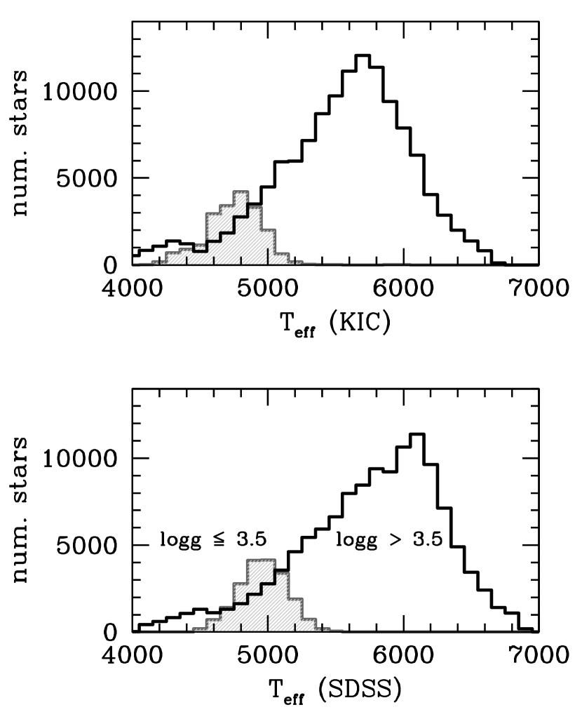
Figure 1.— Long-cadence data from the KIC (top) and with our revised SDSS-based effective temperature scale (bottom). Data are binned in $100$ K increment. Dwarfs with KIC $\log{g}>3.5$ (open histogram) are separated from giants with lower $\log{g}$ (shaded histogram).

For our sample we chose long-cadence targets in the KIC; our initial source had $161,994$ candidates. We selected stars with $griz$ photometry detected in all of the bandpasses. This sample was nearly complete in the 2MASS catalog. We excluded a small number of sources with 2MASS photometry quality flags not equal to AAA ($N=3,602$) and stars with colors outside the range of validity of either the IRFM or SDSS scales ($N=11,830$), leaving us with a main sample of $146,562$ stars. We then further restricted our sample by excluding stars with $\log{g}$ estimates below $3.5$ dex in the KIC ($N=19,663$) for a dwarf comparison sample of $126,899$. We illustrate the distribution of stars in the sample in $100$ K bins in Figure 1, both in the initial catalog (top panel) and the revised one in this paper (bottom panel). We did not use the giants in our comparison of the dwarf-based temperature scale (Section 3), but we do employ theoretical $\log{g}$ corrections to the photometric temperatures for the purposes of the main catalog (see Sections 3.2 and 4.2).

2.2. Recalibration of the KIC Photometry

We adopted three primary color indices ($g\,-\,r$, $g\,-\,i$, and $g\,-\,z$) as our temperature indicators for the SDSS filter system. A preliminary comparison of colors yielded surprising internal differences and trends as a function of mean $T_{\rm eff}$ in the relative temperatures inferred from these color indices (see below). Because the A09 color-color trends were calibrated using SDSS photometry of M67, this reflects a zero-point difference between the KIC and SDSS photometry in the color-color plane. It is not likely that this difference is caused by extinction or stellar population differences because all three colors have similar sensitivities to extinction and metallicity. Initially, we suspected problems with the SDSS calibration (see An et al., 2008, for a discussion of zero-point uncertainties). However, the differences seen were outside of the error bounds for the SDSS photometry. For a fraction of the targets (about $2\%$) the temperatures inferred from different color sources (SDSS versus IRFM from 2MASS colors) are also discordant by more than three standard deviations, in some cases by thousands of degrees in $T_{\rm eff}$. We examine both phenomena below.

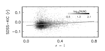
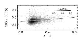
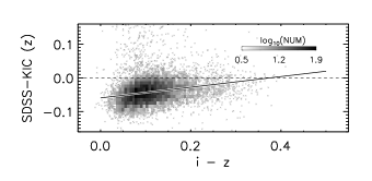
Figure 2.— Photometry comparisons between SDSS (DR8) and the KIC in the sense of the former minus the latter. Comparisons are shown in $griz$ from top to bottom panels. Solid lines are a linear fit to the residuals.

About 10% of the stars in the Kepler field are covered in the most recent data release (DR8) of the SDSS imaging survey (Aihara et al., 2011). There is an overlap in the two photometric sets at $14\lesssim r\lesssim 18$. We compare photometry for stars in common in Figure 2. With a $1\arcsec$ search radius, we found that the median differences (in the sense of the SDSS minus KIC), after rejecting stars with differences greater than $0.2$ mag on both sides, are $\Delta g=-0.040$, $\Delta r=-0.028$, $\Delta i=-0.045$, and $\Delta z=-0.042$.

Inspection of Figure 2 shows that these differences are also functions of color. Solid lines are a linear fit to the data after an iterative $3\sigma$ rejection. The linear transformation equations are as follows:

$$g_{\rm SDSS}=g_{\rm KIC}+0.0921(g\,-\,r)_{\rm KIC}-0.0985,$$ (1)

$$r_{\rm SDSS}=r_{\rm KIC}+0.0548(r\,-\,i)_{\rm KIC}-0.0383,$$ (2)

$$i_{\rm SDSS}=i_{\rm KIC}+0.0696(r\,-\,i)_{\rm KIC}-0.0583,$$ (3)

$$z_{\rm SDSS}=z_{\rm KIC}+0.1587(i\,-\,z)_{\rm KIC}-0.0597,$$ (4)

where the subscripts indicate either SDSS or KIC photometry.

It is possible that the SDSS photometry in the Kepler field has some zero-point shifts with respect to the main SDSS survey database; the SDSS photometry pipeline can fail to work properly if the source density is too high. To check this, we compared the KIC and the DAOPHOT crowded-field photometry (An et al., 2008) in the NGC 6791 field. Although the sample size is smaller, a comparison of DAOPHOT and KIC photometry in the NGC 6791 field yields systematic offsets in the same sense as the field mean in all band passes. Given that the cluster fiducial sequence from DAOPHOT photometry matches that from an independent study (Clem et al., 2008) relatively well (An et al., 2008), it is unlikely that the offsets seen in Figure 2 are due to zero-point issues in the SDSS photometry.

We also checked the standard star photometry in Brown et al. (2011), which is originally from the SDSS DR1 photometry for 284 stars outside of the Kepler field. We compared with the SDSS DR8 photometry, but did not find the aforementioned trends outside of those expected from random photometric errors: the mean differences (SDSS minus KIC values) were $-0.009$, $-0.004$, $+0.004$, and $+0.012$ mag in $griz$, respectively, with an error in the mean of the order of $0.001$ mag. Therefore, revisions of the standard magnitude system (SDSS DR1 versus DR8) do not appear to be the explanation either. We also investigated the possibility of a zero-point difference between the faint and bright stars in the KIC, which had different exposures. However, we found that magnitude offsets with respect to SDSS are similar for both samples, and that the internal dispersion of the KIC temperature estimates is essentially the same with each other. Regardless of the origin, the differences between the SDSS and KIC photometry are present in the overlap sample, and we therefore adjusted the mean photometry to be on the most recent SDSS scale.

Inspection of Figure 2 also reveals another problem in the KIC photometry: a sub-population of stars are much brighter in the KIC than in the SDSS even after photometric zero-point shifts have been accounted for. We do believe that unresolved background stars explains the occasional cases where different colors predict very different temperatures. In Figure 2 there are many data points that have KIC magnitudes brighter than the SDSS ones. We attribute these stars to blended sources in the KIC. The mean FWHM of SDSS images is $1.4\arcsec$, while that of KIC photometry is $2.4\arcsec$.

To check on this possibility, we cross-checked $13,284$ stars in common between DR8 of the SDSS and our KIC sample. $312$ stars had a resolved SDSS source within $2.4\arcsec$, while $20$ have two or more such blended sources. $2.5\%$ of the stars would therefore have resolved blends between the resolution of the two surveys. If we assume that the space density of blends is constant, we can use the density of blends to estimate the fraction present even in the higher resolution SDSS sample. When this effect is accounted for, we would expect $3.8\%$ of the KIC sources to have a blended star within the resolution limit of the KIC. The average such star was $2.85$ mag fainter than the KIC target, sufficient to cause a significant anomaly in the inferred color-temperature relationships. A comparable fraction of the catalog is likely to have similar issues. A significant contribution from background stars would in general combine light from stars with different temperatures. As a result, one would expect different color-temperature relations to predict discordant values. We therefore assess the internal consistency of the photometric temperatures as a quality control check in our revised catalog to identify possible blends (Section 2.4).

To identify blended sources in the KIC, we further performed a test using the separation index (Stetson et al., 2003), which is defined as the logarithmic ratio of the surface brightness of a star to the summed brightness from all neighboring stars (see also An et al., 2008). However, we found that applying the separation index to the KIC does not necessarily provide unique information for assessing the effects of the source blending.

2.3. Base Model Isochrone

We adopted stellar isochrones in A09 for the estimation of photometric temperatures. Interior models were computed using YREC, and theoretical color-$T_{\rm eff}$ relations were derived from the MARCS stellar atmospheres model: see A09 and An et al. (2009b) for details. These model colors were then calibrated using observed M67 sequences as in our earlier work in the Johnson-Cousins system (Pinsonneault et al., 2003, 2004; An et al., 2007a, b). The empirical color corrections in $ugriz$ were defined using M67 at its solar metallicity, and a linear ramp in [Fe/H] was adopted so that the color corrections become zero at or below [Fe/H]$<-0.8$. Detailed test on the empirical color corrections will be presented elsewhere (An et al. 2012, in preparation).

As a base case of this work, we adopted the mean metallicity recorded in the KIC of [Fe/H]$=-0.2$. This metallicity is comparable to, or slightly below, that in the solar neighborhood. For example, the Geneva-Copenhagen Survey (Nordstrom et al., 2004) has a mean [Fe/H] of $-0.14$ dex with a dispersion of $0.19$ dex; a recent revision by Casagrande et al. (2011) raises the mean [Fe/H] to $-0.07$ dex, which is a fair reflection of the systematic uncertainties. The bulk of the KIC dwarfs are about $100$ pc above the galactic plane, and thus would be expected to have somewhat lower metallicity. In the following analysis, we assumed [Fe/H]$=-0.2$ when using $griz$- or IRFM color-$T_{\rm eff}$ relationships, unless otherwise stated.

Table 1Base Isochrone at [Fe/H]$=-0.2$

Mass/$M_{\odot}$	$T_{\rm eff}$	$\log{L/L_{\odot}}$	$\log{g}$	$M_{r}$	$g\,-\,r$	$g\,-\,i$	$g\,-\,z$
$1.50$	$7506.2$	$0.85$	$4.22$	$2.60$	$0.032$	$-0.022$	$-0.111$
$1.46$	$7409.2$	$0.81$	$4.23$	$2.70$	$0.051$	$0.007$	$-0.076$
$1.43$	$7306.3$	$0.76$	$4.24$	$2.80$	$0.070$	$0.038$	$-0.039$
$1.40$	$7200.2$	$0.72$	$4.25$	$2.90$	$0.091$	$0.069$	$-0.000$
$1.37$	$7091.8$	$0.68$	$4.25$	$3.00$	$0.113$	$0.102$	$0.039$
$1.35$	$6992.9$	$0.64$	$4.26$	$3.10$	$0.133$	$0.132$	$0.076$
$1.32$	$6902.5$	$0.59$	$4.27$	$3.20$	$0.152$	$0.160$	$0.111$
$1.30$	$6817.8$	$0.55$	$4.29$	$3.30$	$0.169$	$0.187$	$0.143$
$1.27$	$6737.8$	$0.51$	$4.30$	$3.40$	$0.186$	$0.212$	$0.175$
$1.25$	$6662.9$	$0.47$	$4.31$	$3.50$	$0.203$	$0.236$	$0.204$
$1.22$	$6592.6$	$0.43$	$4.33$	$3.60$	$0.218$	$0.259$	$0.232$
$1.20$	$6524.8$	$0.39$	$4.34$	$3.70$	$0.234$	$0.281$	$0.259$
$1.18$	$6458.9$	$0.34$	$4.36$	$3.80$	$0.249$	$0.304$	$0.286$
$1.16$	$6394.6$	$0.30$	$4.37$	$3.90$	$0.265$	$0.326$	$0.313$
$1.14$	$6332.4$	$0.26$	$4.39$	$4.00$	$0.280$	$0.347$	$0.339$
$1.12$	$6271.2$	$0.22$	$4.41$	$4.10$	$0.295$	$0.369$	$0.366$
$1.10$	$6210.7$	$0.18$	$4.42$	$4.20$	$0.310$	$0.391$	$0.392$
$1.08$	$6151.0$	$0.14$	$4.44$	$4.30$	$0.326$	$0.413$	$0.418$
$1.06$	$6092.1$	$0.10$	$4.45$	$4.40$	$0.341$	$0.434$	$0.445$
$1.04$	$6033.6$	$0.06$	$4.47$	$4.50$	$0.357$	$0.457$	$0.472$
$1.02$	$5975.0$	$0.02$	$4.49$	$4.60$	$0.373$	$0.479$	$0.498$
$1.00$	$5915.8$	$-0.02$	$4.50$	$4.70$	$0.389$	$0.501$	$0.524$
$0.98$	$5855.5$	$-0.06$	$4.51$	$4.80$	$0.406$	$0.524$	$0.550$
$0.96$	$5793.9$	$-0.10$	$4.53$	$4.90$	$0.423$	$0.548$	$0.579$
$0.95$	$5731.4$	$-0.14$	$4.54$	$5.00$	$0.441$	$0.573$	$0.609$
$0.93$	$5669.8$	$-0.18$	$4.55$	$5.10$	$0.460$	$0.598$	$0.640$
$0.91$	$5606.9$	$-0.22$	$4.56$	$5.20$	$0.479$	$0.625$	$0.672$
$0.90$	$5538.8$	$-0.26$	$4.57$	$5.30$	$0.500$	$0.655$	$0.709$
$0.88$	$5472.0$	$-0.29$	$4.58$	$5.40$	$0.522$	$0.686$	$0.747$
$0.86$	$5406.0$	$-0.33$	$4.59$	$5.50$	$0.545$	$0.717$	$0.785$
$0.85$	$5340.0$	$-0.37$	$4.60$	$5.60$	$0.568$	$0.750$	$0.826$
$0.83$	$5273.8$	$-0.41$	$4.61$	$5.70$	$0.593$	$0.785$	$0.869$
$0.82$	$5207.7$	$-0.44$	$4.61$	$5.80$	$0.619$	$0.822$	$0.914$
$0.81$	$5142.1$	$-0.48$	$4.62$	$5.90$	$0.647$	$0.861$	$0.961$
$0.79$	$5077.2$	$-0.51$	$4.63$	$6.00$	$0.676$	$0.901$	$1.010$
$0.78$	$5013.1$	$-0.55$	$4.63$	$6.10$	$0.707$	$0.943$	$1.061$
$0.77$	$4949.9$	$-0.58$	$4.64$	$6.20$	$0.739$	$0.987$	$1.115$
$0.75$	$4887.6$	$-0.62$	$4.64$	$6.30$	$0.773$	$1.034$	$1.170$
$0.74$	$4826.3$	$-0.65$	$4.65$	$6.40$	$0.808$	$1.082$	$1.228$
$0.73$	$4766.1$	$-0.68$	$4.65$	$6.50$	$0.846$	$1.132$	$1.288$
$0.72$	$4707.4$	$-0.72$	$4.66$	$6.60$	$0.885$	$1.185$	$1.350$
$0.71$	$4650.3$	$-0.75$	$4.66$	$6.70$	$0.926$	$1.239$	$1.414$
$0.70$	$4595.1$	$-0.78$	$4.66$	$6.80$	$0.967$	$1.295$	$1.479$
$0.69$	$4541.8$	$-0.81$	$4.67$	$6.90$	$1.007$	$1.350$	$1.544$
$0.68$	$4490.6$	$-0.84$	$4.67$	$7.00$	$1.047$	$1.406$	$1.610$
$0.67$	$4441.5$	$-0.87$	$4.68$	$7.10$	$1.084$	$1.461$	$1.675$
$0.66$	$4394.5$	$-0.90$	$4.68$	$7.20$	$1.121$	$1.515$	$1.740$
$0.65$	$4349.3$	$-0.93$	$4.69$	$7.30$	$1.155$	$1.568$	$1.804$
$0.64$	$4306.0$	$-0.96$	$4.69$	$7.40$	$1.188$	$1.619$	$1.867$
$0.63$	$4264.4$	$-0.99$	$4.70$	$7.50$	$1.218$	$1.670$	$1.928$
$0.62$	$4224.3$	$-1.02$	$4.70$	$7.60$	$1.247$	$1.719$	$1.989$
$0.61$	$4185.9$	$-1.04$	$4.71$	$7.70$	$1.273$	$1.766$	$2.048$
$0.60$	$4148.9$	$-1.07$	$4.71$	$7.80$	$1.298$	$1.812$	$2.105$
$0.59$	$4113.7$	$-1.10$	$4.72$	$7.90$	$1.320$	$1.856$	$2.160$
$0.58$	$4079.8$	$-1.13$	$4.73$	$8.00$	$1.340$	$1.898$	$2.213$
$0.58$	$4047.1$	$-1.16$	$4.74$	$8.10$	$1.358$	$1.939$	$2.265$

Table 1 shows our base model isochrone at [Fe/H]$=-0.2$ and the age of $1$ Gyr. All colors are color-calibrated as described above. Note that the isochrone calibration is defined for the main-sequence only; the relevant corrections for the lower gravities of evolved stars are described separately in Section 3.2. The SDSS photometry did not cover the main-sequence turn-off region of M67 because of the brightness limit in the SDSS imaging survey at $r\sim 14$ mag. As a result, the M67-based $griz$ color calibration is strictly valid at $4000\leq T_{\rm eff}\leq 6000$ K (see Figure $17$ in A09).

The choice of $1$ Gyr age in our base model isochrone has a negligible effect on the color-$T_{\rm eff}$ relations. The difference between $1$ Gyr and $12$ Gyr isochrones is only less than $5$ K near main-sequence turn-off. However, younger age of the models enables the determination of photometric $T_{\rm eff}$ over a wider range of colors at the hot $T_{\rm eff}$ end.

Table 2Coefficients for Polynomial Color-$T_{\rm eff}$ Relations

Coeff.	$g\,-\,r$	$g\,-\,i$	$g\,-\,z$
$a_{0}$	$0.6676$	$0.6888$	$0.7053$
$a_{1}$	$0.3434$	$0.2012$	$0.2022$
$a_{2}$	$0.5851$	$0.4518$	$0.2733$
$a_{3}$	$-0.6919$	$-0.4871$	$-0.2844$
$a_{4}$	$0.1445$	$0.1926$	$0.1079$
$a_{5}$	$0.0594$	$-0.0256$	$-0.0144$

Note. — Coefficients in equation 5. These cofficients are valid at $4080\leq T_{\rm eff}<7000$ K, or $0.13<(g\,-\,r)_{0}<1.34$, $0.13<(g\,-\,i)_{0}<1.90$, and $0.07<(g\,-\,z)_{0}<2.21$, respectively.

From Table 1 we derived polynomial color-$T_{\rm eff}$ relations of our base model for convenience of use. The following relationship was used over the temperature range $4080$ K $\leq T_{\rm eff}{\rm(YREC)}<7000~{}K$:

$$5040/T_{\rm eff}=a_{0}+a_{1}x+a_{2}x^{2}+a_{3}x^{3}+a_{4}x^{4}+a_{5}x^{5}$$ (5)

where $x$ represents $g\,-\,r$, $g\,-\,i$, or $g\,-\,z$, and $a_{0}$–$a_{5}$ are coefficients for each color index as listed in Table 2. Difference in $T_{\rm eff}$ inferred from these polynomial equations compared to those found in Table 1 from interpolation in the full tables are at or below the $6$ K level.

Table 3$T_{\rm eff}$ Corrections for Different [Fe/H]

	[Fe/H]
color	$-2.0$	$-1.5$	$-1.0$	$-0.6$	$-0.4$	$-0.2$	$+0.0$	$+0.2$	$+0.4$
$g\,-\,r$
$0.1$	$44$	$36$	$20$	$19$	$7$	$0$	$0$	$\cdots$	$\cdots$
$0.2$	$-32$	$-32$	$-27$	$-6$	$-4$	$0$	$20$	$61$	$100$
$0.3$	$-120$	$-103$	$-74$	$-33$	$-20$	$0$	$33$	$84$	$145$
$0.4$	$-162$	$-144$	$-110$	$-60$	$-32$	$0$	$44$	$104$	$176$
$0.5$	$-168$	$-165$	$-130$	$-75$	$-42$	$0$	$44$	$116$	$194$
$0.6$	$-186$	$-185$	$-144$	$-80$	$-42$	$0$	$46$	$113$	$192$
$0.7$	$-214$	$-195$	$-149$	$-84$	$-44$	$0$	$48$	$104$	$178$
$0.8$	$-238$	$-198$	$-149$	$-85$	$-42$	$0$	$45$	$97$	$157$
$0.9$	$-262$	$-204$	$-153$	$-86$	$-43$	$0$	$44$	$83$	$131$
$1.0$	$-282$	$-212$	$-160$	$-94$	$-46$	$0$	$45$	$77$	$113$
$1.1$	$-289$	$-223$	$-174$	$-107$	$-51$	$0$	$45$	$69$	$93$
$1.2$	$\cdots$	$-233$	$-207$	$-136$	$-60$	$0$	$42$	$45$	$28$
$1.3$	$\cdots$	$\cdots$	$\cdots$	$\cdots$	$-83$	$0$	$37$	$-33$	$\cdots$
$g\,-\,i$
$0.1$	$86$	$67$	$33$	$20$	$9$	$0$	$-5$	$-23$	$\cdots$
$0.3$	$5$	$-3$	$-13$	$-5$	$-3$	$0$	$16$	$35$	$61$
$0.5$	$-69$	$-70$	$-61$	$-37$	$-21$	$0$	$27$	$63$	$108$
$0.7$	$-84$	$-99$	$-88$	$-52$	$-27$	$0$	$33$	$75$	$127$
$0.9$	$-126$	$-142$	$-118$	$-65$	$-34$	$0$	$35$	$75$	$125$
$1.1$	$-168$	$-156$	$-128$	$-72$	$-36$	$0$	$39$	$71$	$112$
$1.3$	$-204$	$-166$	$-134$	$-78$	$-40$	$0$	$41$	$68$	$99$
$1.5$	$-233$	$-180$	$-143$	$-83$	$-42$	$0$	$44$	$68$	$95$
$1.7$	$\cdots$	$-206$	$-172$	$-95$	$-47$	$0$	$50$	$70$	$93$
$1.9$	$\cdots$	$\cdots$	$\cdots$	$\cdots$	$-56$	$0$	$61$	$80$	$101$
$g\,-\,z$
$0.1$	$94$	$68$	$33$	$15$	$6$	$0$	$-4$	$-16$	$\cdots$
$0.3$	$45$	$25$	$2$	$-1$	$0$	$0$	$10$	$19$	$33$
$0.5$	$-11$	$-23$	$-35$	$-24$	$-13$	$0$	$20$	$41$	$72$
$0.7$	$-27$	$-43$	$-47$	$-29$	$-17$	$0$	$20$	$50$	$87$
$0.9$	$-63$	$-84$	$-78$	$-46$	$-23$	$0$	$26$	$54$	$92$
$1.1$	$-109$	$-119$	$-102$	$-59$	$-29$	$0$	$31$	$60$	$93$
$1.3$	$-145$	$-137$	$-116$	$-66$	$-34$	$0$	$35$	$60$	$90$
$1.5$	$-177$	$-147$	$-121$	$-70$	$-36$	$0$	$39$	$61$	$87$
$1.7$	$-205$	$-160$	$-128$	$-73$	$-36$	$0$	$44$	$66$	$92$
$1.9$	$-225$	$-182$	$-144$	$-77$	$-39$	$0$	$49$	$72$	$97$
$2.1$	$\cdots$	$\cdots$	$\cdots$	$-87$	$-44$	$0$	$58$	$82$	$109$

Note. — The sense of the difference is the model $T_{\rm eff}$ at a given [Fe/H] minus that of the fiducial metallicity, [Fe/H]$=-0.2$. The $T_{\rm eff}$ at a fixed color generally becomes cooler at a lower [Fe/H]. In other words, the above correction factor should be added to the SDSS $T_{\rm eff}$, if the metallicity effects should be taken into account.

In Table 3 we provide the metallicity sensitivity of the color-$T_{\rm eff}$ relations in the model isochrones at several [Fe/H]. To generate this table, we compared $1$ Gyr old isochrones at individual [Fe/H] with our fiducial model (Table 1) at [Fe/H]$=-0.2$ for each color index, and estimated the $T_{\rm eff}$ difference at a given color (individual models minus the fiducial isochrone). We include the sensitivity to metallicity predicted by atmospheres models, but do not include an additional empirical correction below [Fe/H]$=-0.8$ because the cluster data did not require one. The $T_{\rm eff}$ at a fixed color generally becomes cooler at a lower [Fe/H]. We use the metallicity corrections in the comparisons with spectroscopic $T_{\rm eff}$ where we have reliable [Fe/H] measurements (see Section 3.4), but do not apply corrections to the KIC sample (see Sections 3.1 and 4.2).

2.4. Photometric $T_{\rm eff}$ Estimation

The stellar parameters for the KIC were generated using a Bayesian method (see Brown et al., 2011, for a discussion). We adopt a less ambitious approach focused on KIC stars identified as dwarfs. The three key assumptions in our work are that we define $T_{\rm eff}$ at a reference [Fe/H] and the model $\log{g}$ (Table 1), and that we adopt the map-based E$(B\,-\,V)$ in the KIC as a prior. Within this framework we can then derive independent temperature estimates from the $griz$ photometry and infer the random $T_{\rm eff}$ errors. Uncertainties in the extinction, the impact on the colors of unresolved binaries, and population (metallicity and $\log{g}$) differences can then be treated as error sources. In the latter case, we can compute correction terms to be used if there is an independent method of measurement. This approach is not the same as the one that we have employed in earlier studies, so a brief justification is in order.

The traditional approach to photometric parameter estimation is to take advantage of the fact that different filter combinations respond to changes in metallicity and extinction. If one has the proper template metallicity and extinction, for example, the answers from the various colors will agree within photometric errors; if not, the pattern of differences can be used to solve for them (see An et al., 2007a, b).

The particular problem for the KIC is that the available color combinations in $griz$ are rather insensitive to both over the narrow metallicity range and the modest mean extinctions ($0\lesssim E(B\,-\,V)\lesssim 0.2$) in the field (see An et al., 2009b, for a discussion of $griz$-based estimates). In other words, all the color combinations in $griz$ produce similar metallicity sensitivities of color-$T_{\rm eff}$ relations. Therefore, even though the absolute change of photometric $T_{\rm eff}$ can be significant by the error in the adopted metallicity, it is difficult to infer photometric metallicities based on the available filter combinations in $griz$ alone.

The temperature estimates in Lejeune et al. (1997, 1998), which were used as the basis color-$T_{\rm eff}$ relations in our prior color calibration in the Johnson-Cousins system (An et al., 2007a, b), are insensitive to $\log{g}$ near the main sequence, and the IRFM scale in C10 does not include an explicit $\log{g}$ dependence for the temperatures. As a result, we believe that the most fruitful approach is to define a benchmark temperature estimate. If additional color information or spectroscopic [Fe/H] data become available, the relevant corrections can be applied, and we present methods below to do so (Section 3).

The KIC gravities for cool stars are precise enough to separate dwarfs (KIC $\log{g}>3.5$) from giants (KIC $\log{g}\leq 3.5$) and to be used as a basis for corrections to the temperatures for giant stars (Sections 3.2 and 4.2). The KIC metallicities are more problematic, and we do not use them for temperature corrections. Instead the metallicity sensitivity is included as an error source in our effective temperature estimates.

We adopted the map-based KIC catalog extinction estimates ($A_{V}$) and the Cardelli et al. (1989) standard extinction curves with $A_{V}=3.1E(B\,-\,V)$. Extinction coefficients in $griz$ were derived in A09: $A_{g}=1.196A_{V}$ , $A_{r}=0.874A_{V}$ , $A_{i}=0.672A_{V}$, and $A_{z}=0.488A_{V}$. We further took $A_{J}=0.282A_{V}$, $A_{H}=0.180A_{V}$, $A_{K_{s}}=0.117A_{V}$, and $A_{V_{T}}=1.050A_{V}$, where $V_{T}$ represents the Tycho $V$ passband (An et al., 2007a).

For a given extinction-corrected set of $griz$ magnitudes, we searched the best-fitting stellar template in the model isochrone for each star in the KIC. The mean $T_{\rm eff}$ was obtained by simultaneously fitting the models in $griz$, assuming $0.01$ mag error in $gri$ and $0.03$ mag error in $z$. We also estimated $T_{\rm eff}$ using the same model isochrone, but based on data from each of our fundamental color indices ($g\,-\,r$, $g\,-\,i$, and $g\,-\,z$), which is simply a photometric $T_{\rm eff}$ estimation from a single color-$T_{\rm eff}$ relation. Its purpose is to readily identify and quantify the internal consistency of our primary temperature determination from the multi-color-$T_{\rm eff}$ space.

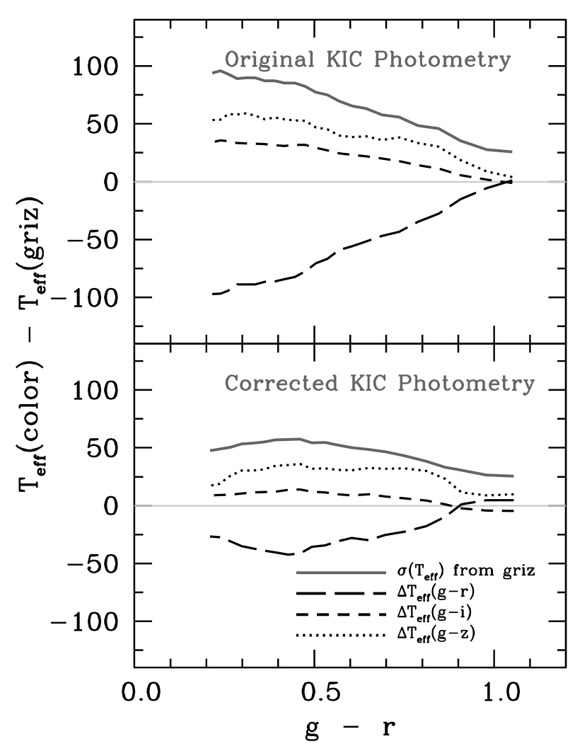
Figure 3.— Internal dispersion in $T_{\rm eff}$ estimates (solid line) and differences between the mean $griz$-based $T_{\rm eff}$ and that inferred from $g\,-\,r$ (long-dashed), $g\,-\,i$ (short-dashed), and $g\,-\,z$ (dotted). Original KIC photometry is used in the top panel, while corrected KIC photometry is used in the bottom panel.

In Figure 3 we plot the internal dispersion and the mean trends of $T_{\rm eff}$ from a given color index with respect to the average error-weighted temperature from $griz$ for all of the dwarfs in our sample. The top panel shows the case of the original KIC data, and the bottom panel shows the one for the corrected KIC photometry. The magnitude corrections described in Section 2.2 were motivated by concordance between SDSS and the KIC. Nevertheless, the results when using the recalibrated KIC photometry as temperature indicators were extremely encouraging.

Although the internal agreement is not complete, the remaining differences in the bottom panel of Figure 3 are comparable to the zero-point uncertainties discussed in An et al. (2008). We view this as strong supporting evidence for the physical reality of the magnitude corrections illustrated in Figure 2. We therefore recommend that the zero-points of the KIC photometry be modified according to equations 1–4. In the remainder of the paper, we use magnitudes and colors adjusted using these equations.

3. Revised $T_{\rm eff}$ Scale for the KIC

We begin by evaluating the $T_{\rm eff}$ inferred from the IRFM and the SDSS systems for dwarfs (KIC $\log{g}>3.5$). We then use open clusters and comparisons with high-resolution spectroscopy to establish agreement between the two scales, indicating the need for correction to the KIC effective temperatures. We then evaluate the impact of binaries, surface gravity, and metallicity on the colors. We provide statistical corrections to the temperatures caused by unresolved binary companions, as well as corrections for $\log{g}$ and metallicity. We then perform a global error analysis including extinction uncertainties and the mild metallicity dependence of our color-temperature relationships. The latter is treated as a temperature error source because we evaluate all KIC stars at a mean reference metallicity ([Fe/H]$=-0.2$).

3.1. Temperature scale comparisons for dwarfs

We have three native temperature scales to compare: the one in the KIC, our isochrone-based scale from $griz$ (hereafter SDSS or $griz$-based scale unless otherwise stated), and one from the ($J\,-\,K_{s}$)-based IRFM. Below we compare the mean differences between them and compare the dispersions to those expected from random error sources alone. We find an offset between the KIC and the other two scales. The IRFM and SDSS scales are closer, but some systematic differences between them are also identified. In this section, we examine various effects that could be responsible for these differences, and finish with an overall evaluation of the error budget.

We computed IRFM and SDSS $T_{\rm eff}$ estimates assuming [Fe/H]$=-0.2$. In terms of the temperature zero-point, adopting this metallicity led to mean shifts of $+20$ K in $J\,-\,K_{s}$, and $-40$ K in the $griz$-based $T_{\rm eff}$ estimate, relative to those which would have been obtained with solar abundance. In other words, changes in the adopted mean metallicity would cause zero-point shifts of $\sim 60$ K in the overall $T_{\rm eff}$ scale comparison. On the other hand, a scatter around the mean metallicity in the Kepler field is another source of error that would make the observed $T_{\rm eff}$ comparison broader. We discuss this in Section 3.6 along with other sources of uncertainties.

In the comparisons below we repeatedly clipped the samples, rejecting stars with temperature estimates more than three standard deviations from the mean, until we achieved convergence. This typically involved excluding about 1 % of the sample. Such stars represent cases where the extinction corrections break down or where the relative colors differ drastically from those expected for single unblended stars.

Random errors were taken from the photometric errors alone and yield a minimum error in temperature. For the SDSS colors we also computed the internal dispersion in the three temperature estimates from $g\,-\,r$, $g\,-\,i$, and $g\,-\,z$, and used the larger of either this dispersion or the one induced by photometric errors as a random uncertainty. Median random errors for the SDSS and IRFM temperatures were $40$ K and $171$ K, respectively. These estimates are consistent with expectations from the observed dispersions of the colors (see Figure 17). We then compared stars at fixed KIC temperature and computed the average $T_{\rm eff}$ difference between those inferred from the IRFM, those inferred from $griz$, and the scale in the KIC itself. For a limited subset of stars, we also had Tycho photometry, and computed temperatures from $V_{T}\,-\,K_{s}$. This sample is small, so we used it as a secondary temperature diagnostic.

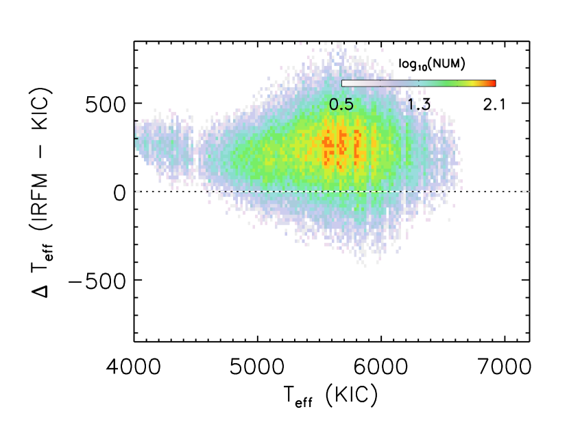
Figure 4.— Comparisons of the temperatures inferred from IRFM ($J\,-\,K_{s}$) as a function of KIC $T_{\rm eff}$. The color coding indicates the logarithmic number density of stars with a temperature and temperature difference at the indicated point (see legend).

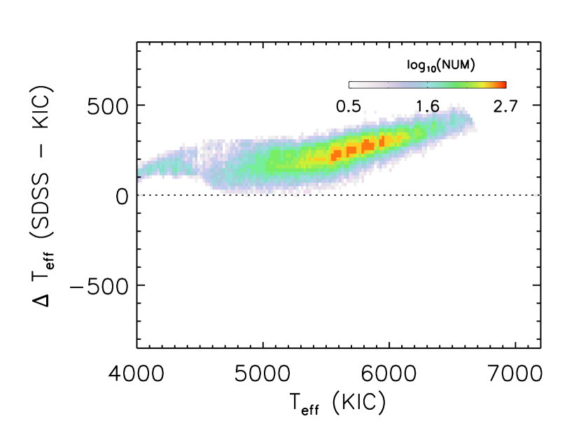
Figure 5.— Same as in Figure 4, but from $griz$ colors.

In Figures 4–5 we illustrate the differences between KIC and the IRFM and SDSS, respectively. For the IRFM scale in Figure 4, we compare $T_{\rm eff}$ from $J\,-\,K_{s}$. In Figure 5 we compare the mean SDSS temperatures inferred from $griz$ to that in the KIC. In both cases we see a significant zero-point shift, indicating a discrepancy between the fundamental effective temperature scale and that adopted by the KIC.

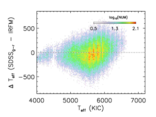
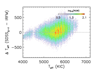
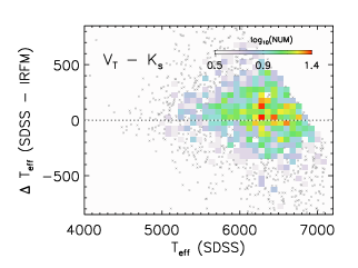
Figure 6.— Differences in $T_{\rm eff}$ between the IRFM and SDSS scales as a function of KIC $T_{\rm eff}$: $T_{\rm eff}(g\,-\,r)$ vs. $T_{\rm eff}(J\,-\,K_{s})$ (upper left); $T_{\rm eff}(g\,-\,i)$ vs. $T_{\rm eff}(J\,-\,K_{s})$ (upper right); $T_{\rm eff}(g\,-\,z)$ vs. $T_{\rm eff}(J\,-\,K_{s})$ (lower left); $T_{\rm eff}(griz)$ vs. $T_{\rm eff}(V_{T}\,-\,K_{s})$ (lower right). The color coding defines the logarithmic number density of points with the indicated temperature and temperature difference (see legend for details).

The $T_{\rm eff}$ from the IRFM and the SDSS from individual color indices ($g\,-\,r$, $g\,-\,i$, and $g\,-\,z$) are compared in Figure 6. The IRFM scale for the Tycho $V_{T}$ and 2MASS $K_{s}$ is used in the bottom right panel. The central result (that the KIC scale is too cool) is robust, and can also be seen in comparisons with high-resolution spectroscopic temperature estimates (see Section 3.4 below). In Section 4.2 we provide quantitative tabular information on the statistical properties of the sample.

The two fundamental scales (IRFM and SDSS) are close, but not identical, for cooler stars; they deviate from one another and the KIC above $6000$ K (on the SDSS scale). As discussed in Section 3.6 below, the total internal dispersion in the $griz$ temperature estimates is also consistently larger for cool stars than that expected from random photometric uncertainties alone, and there are modest but real offsets between the two fundamental scales even for cool stars. We therefore need to understand the origin of these differences and to quantify the random and systematic uncertainties in our temperature estimates.

Open clusters provide a good controlled environment for testing the concordance of the SDSS and IRFM scales. The SDSS scale was developed to be consistent with Johnson-Cousins-based temperature calibrations in open clusters, so a comparison of the An et al. and IRFM Johnson-Cousins systems in clusters will permit us to verify their underlying agreement. As we show below, the two scales are close for cool stars when $B\,-\,V$, $V\,-\,I_{C}$, or $V\,-\,K_{s}$ indices are employed in the temperature determinations, but exhibit modest but real systematics for the hotter stars. The IRFM relation in $J\,-\,K_{s}$, on the other hand, is found to have a systematic difference from those of these optical-2MASS indices. For the reasons discussed in the following section, we therefore adopt a correction to our SDSS temperatures for hot stars, making the two photometric systems consistent.

We can also check our methodology against spectroscopic temperature estimates, and need to consider uncertainties from extinction, binary companions, and metallicity. We therefore begin by defining an extension of our method to giants, which can be checked against spectroscopy. We then look at open cluster tests, spectroscopic tests, binary effects, and the overall error budget.

3.2. Tests of the temperature scale for giants

Our YREC $T_{\rm eff}$ estimates are based on calibrated isochrones (Table 1), which do not include evolved stars. About $14\%$ of the KIC sample are giants and subgiants with $\log{g}\leq 3.5$ as estimated in the KIC, so a reliable method for assigning effective temperatures to such stars is highly desirable. Fortunately, this is feasible because the color-temperature relations for the bulk of the long cadence targets are not strong functions of surface gravity. For the purposes of the catalog we therefore supplement the fundamental dwarf scale with theoretical corrections for the effect of surface gravity on the colors.

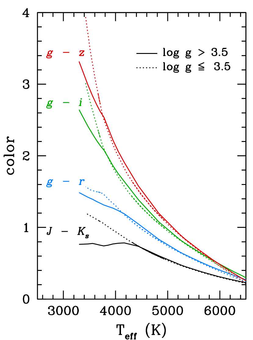
Figure 7.— Main-sequence (solid; $\log{g}>3.5$) and post-main-sequence (dashed; $\log{g}\leq 3.5$) color-temperature relationships for models along a $1$ Gyr isochrone with solar composition are shown for illustrative purposes. Colors illustrated are $g\,-\,z$, $g\,-\,i$, $g\,-\,r$, and $J\,-\,K_{s}$ (from top to bottom).

Theoretical model atmospheres can be used to quantify the $\log{g}$ dependence of the color-temperature relations by comparing the spectral energy distributions of dwarfs and giants. Figure 7 shows color-temperature relations along a $1$ Gyr solar abundance isochrone for $g\,-\,r$, $g\,-\,i$, $g\,-\,z$, and $J\,-\,K_{s}$ for illustrative purposes. The model isochrone was taken from the web interface of the Padova isochrone database (Girardi et al., 2002; Marigo et al., 2008). As seen in Figure 7 the model color-$T_{\rm eff}$ relations are moderately dependent on $\log{g}$, and illustrate that our photometric $T_{\rm eff}$ needs to be adjusted for giants.

We corrected for the difference in $\log{g}$ by taking theoretical $\log{g}$ sensitivities in $griz$ colors from the ATLAS9 model atmosphere (Castelli & Kurucz, 2004). The choice of these models seems internally inconsistent with our basis model isochrone with MARCS-based colors. Nevertheless, we adopted the ATLAS9 $\log{g}$-color relations, primarily because our cluster-based empirical calibration of the color-$T_{\rm eff}$ relations has not been performed for subgiant and giant branches due to significant uncertainties in the underlying stellar interior models at these evolved stages. Therefore, it is just a matter of choice to adopt the ATLAS9 color tables instead of that of MARCS. Since we generated MARCS color tables in An et al. (2009a) with a specific set of model parameters for dwarfs ($\log{g}\geq 3.5$), we simply opted to take the ATLAS9 colors, and estimate a relative sensitivity of theoretical $\log{g}$-color relations.

We convolved synthetic spectra with the SDSS $griz$ filter response curves, and integrated flux with weights given by photon counts (Girardi et al., 2002). Magnitudes were then put onto the AB magnitude system using a flat $3631$ Jy spectrum (Oke & Gunn, 1983). We created a table with synthetic colors from $\log{g}=0.0$ to $5.0$ dex with a $0.5$ dex increment, and from $4000$ K to $6000$ K with a $250$ K increment at [M/H]=$-1.0$, $-0.5$, $+0.0$, and $+0.2$. Because YREC $T_{\rm eff}$ values were estimated at the fiducial metallicity, [Fe/H]$=-0.2$, we interpolated the color table to obtain synthetic colors at this metallicity. Note that Castelli & Kurucz (2004) adopted the solar mixture of Grevesse & Sauval (1998), as in our YREC isochrone models (A09), so we assumed [M/H] in Castelli & Kurucz (2004) is the same as the [Fe/H] value.

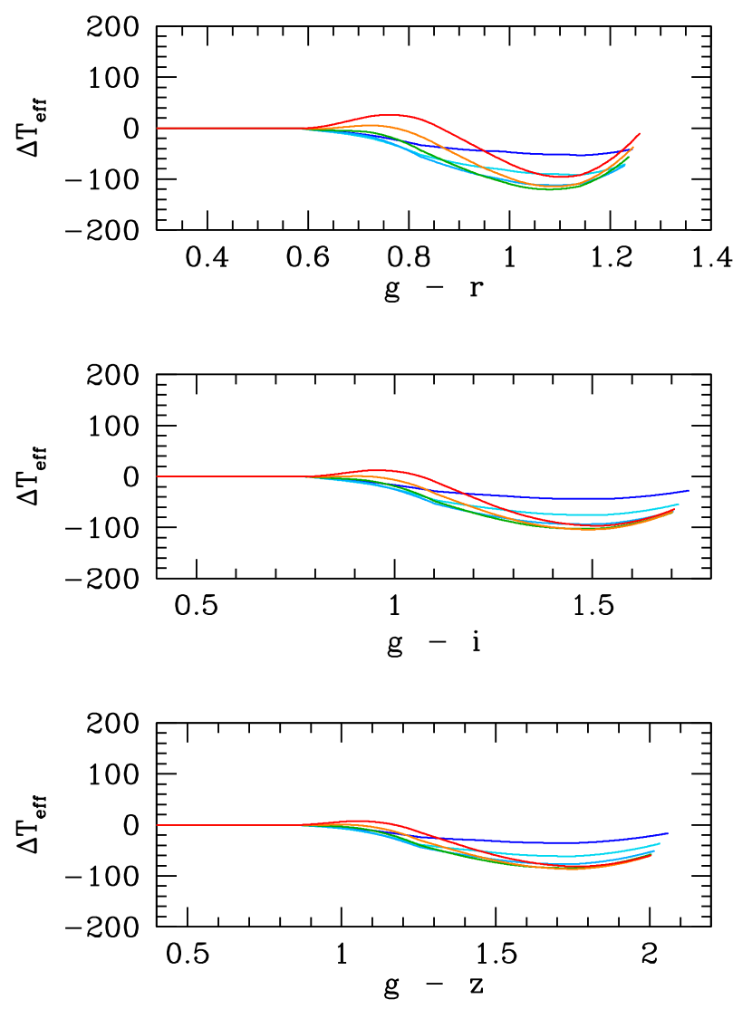
Figure 8.— Theoretical $T_{\rm eff}$ corrections for various $\Delta\log{g}$ values with respect to the fiducial isochrones. Corrections from $\Delta\log{g}=0.5$ to $\Delta\log{g}=3.0$ with a $0.5$ dex increment are shown. A linear ramp was used to define smoothly varying $\Delta T_{\rm eff}$ over $4800<T_{\rm eff}<5800$ K. The sense is that giants with lower $\log{g}$ than the base isochrone tend to have lower $T_{\rm eff}$.

Figure 8 shows the correction factors in $T_{\rm eff}$ as computed from synthetic colors as a function of colors in $g\,-\,r$, $g\,-\,i$, and $g\,-\,z$. We used our base isochrone to compute $\Delta T_{\rm eff}$ at $\Delta\log{g}=0.5$, $1.0$, $1.5$, $2.0$, $2.5$, and $3.0$ dex, where $\Delta\log{g}$ represents the difference between YREC $\log{g}$ and the $\log{g}$ in the KIC. The sense of $\Delta T_{\rm eff}$ is that giants with lower $\log{g}$ than the base model generally tend to have lower $T_{\rm eff}$ than main-sequence dwarfs in the color range considered in this work.

Table 4$\log{g}$ Corrections

		Ref.	$\Delta\log{g}$
$g-r$	$g-i$/$g-z$	$\log{g}$	$0.5$	$1.0$	$1.5$	$2.0$	$2.5$	$3.0$
$\Delta T_{\rm eff}$ from $g-r$
$0.50$	$\cdots$	$4.57$	$0.0$	$0.0$	$0.0$	$0.0$	$0.0$	$0.0$
$0.55$	$\cdots$	$4.59$	$0.0$	$0.0$	$0.0$	$0.0$	$0.0$	$0.0$
$0.60$	$\cdots$	$4.61$	$1.5$	$2.3$	$2.4$	$2.0$	$1.2$	$-0.2$
$0.65$	$\cdots$	$4.62$	$5.8$	$8.1$	$7.3$	$4.5$	$-0.2$	$-7.3$
$0.70$	$\cdots$	$4.63$	$11.2$	$15.3$	$12.9$	$6.1$	$-4.4$	$-18.5$
$0.75$	$\cdots$	$4.64$	$18.5$	$26.7$	$24.6$	$14.0$	$-3.8$	$-25.8$
$0.80$	$\cdots$	$4.65$	$28.2$	$43.2$	$44.3$	$31.6$	$7.3$	$-22.8$
$0.85$	$\cdots$	$4.65$	$36.2$	$58.6$	$65.1$	$55.1$	$28.9$	$-6.7$
$0.90$	$\cdots$	$4.66$	$41.2$	$69.3$	$81.1$	$76.4$	$54.4$	$19.1$
$0.95$	$\cdots$	$4.66$	$44.6$	$77.2$	$93.7$	$94.8$	$78.5$	$45.3$
$1.00$	$\cdots$	$4.67$	$47.1$	$83.4$	$103.8$	$109.3$	$97.9$	$69.8$
$1.05$	$\cdots$	$4.67$	$50.6$	$88.9$	$110.8$	$118.8$	$111.4$	$88.2$
$1.10$	$\cdots$	$4.68$	$51.5$	$90.4$	$111.8$	$119.4$	$114.0$	$95.5$
$1.15$	$\cdots$	$4.69$	$53.1$	$90.2$	$106.4$	$109.7$	$104.0$	$88.4$
$1.20$	$\cdots$	$4.69$	$48.4$	$80.1$	$88.0$	$84.0$	$76.0$	$62.0$
$\Delta T_{\rm eff}$ from $g-i$
$0.50$	$0.655$	$4.57$	$0.0$	$0.0$	$0.0$	$0.0$	$0.0$	$0.0$
$0.55$	$0.725$	$4.59$	$0.0$	$0.0$	$0.0$	$0.0$	$0.0$	$0.0$
$0.60$	$0.795$	$4.61$	$1.2$	$1.9$	$1.8$	$1.4$	$0.6$	$-0.5$
$0.65$	$0.865$	$4.62$	$5.2$	$7.5$	$6.6$	$4.0$	$-0.2$	$-6.0$
$0.70$	$0.934$	$4.63$	$10.3$	$14.5$	$13.2$	$8.2$	$-0.4$	$-12.0$
$0.75$	$1.003$	$4.64$	$16.9$	$25.2$	$25.8$	$19.4$	$7.0$	$-10.3$
$0.80$	$1.071$	$4.65$	$24.7$	$38.7$	$43.4$	$37.3$	$22.4$	$0.8$
$0.85$	$1.138$	$4.65$	$31.1$	$50.8$	$60.1$	$57.1$	$43.4$	$21.5$
$0.90$	$1.205$	$4.66$	$34.9$	$58.6$	$71.4$	$72.3$	$61.9$	$42.8$
$0.95$	$1.272$	$4.66$	$37.9$	$65.1$	$80.7$	$85.2$	$78.6$	$63.0$
$1.00$	$1.341$	$4.67$	$41.3$	$70.9$	$88.3$	$95.4$	$92.1$	$79.3$
$1.05$	$1.411$	$4.67$	$43.4$	$74.3$	$92.5$	$101.1$	$100.6$	$90.4$
$1.10$	$1.483$	$4.68$	$43.8$	$75.3$	$93.6$	$102.7$	$103.9$	$95.9$
$1.15$	$1.559$	$4.69$	$43.1$	$73.7$	$90.8$	$98.7$	$100.4$	$94.2$
$1.20$	$1.639$	$4.69$	$38.3$	$66.2$	$80.6$	$85.9$	$86.7$	$82.0$
$\Delta T_{\rm eff}$ from $g-z$
$0.50$	$0.708$	$4.57$	$0.0$	$0.0$	$0.0$	$0.0$	$0.0$	$0.0$
$0.55$	$0.795$	$4.59$	$0.0$	$0.0$	$0.0$	$0.0$	$0.0$	$0.0$
$0.60$	$0.881$	$4.61$	$0.8$	$1.2$	$1.1$	$0.9$	$0.4$	$-0.4$
$0.65$	$0.966$	$4.62$	$3.6$	$5.1$	$4.4$	$2.5$	$-0.3$	$-4.4$
$0.70$	$1.050$	$4.63$	$7.7$	$11.2$	$10.1$	$6.2$	$0.5$	$-7.5$
$0.75$	$1.133$	$4.64$	$13.5$	$20.6$	$20.7$	$15.6$	$7.5$	$-4.2$
$0.80$	$1.215$	$4.65$	$20.4$	$32.5$	$35.5$	$30.6$	$21.0$	$6.4$
$0.85$	$1.294$	$4.65$	$25.5$	$41.7$	$48.3$	$46.5$	$37.4$	$22.5$
$0.90$	$1.373$	$4.66$	$28.1$	$46.9$	$56.5$	$58.3$	$50.9$	$37.4$
$0.95$	$1.452$	$4.66$	$30.2$	$51.5$	$63.8$	$68.4$	$63.3$	$51.8$
$1.00$	$1.533$	$4.67$	$33.0$	$56.5$	$70.5$	$76.7$	$74.0$	$64.3$
$1.05$	$1.616$	$4.67$	$34.8$	$59.9$	$74.9$	$82.2$	$81.7$	$73.9$
$1.10$	$1.703$	$4.68$	$35.4$	$61.3$	$76.7$	$84.6$	$85.9$	$80.0$
$1.15$	$1.794$	$4.69$	$34.6$	$60.0$	$75.2$	$83.1$	$85.4$	$81.2$
$1.20$	$1.891$	$4.69$	$30.3$	$53.7$	$67.8$	$74.9$	$77.6$	$75.2$

Note. — The sense of the difference is that a positive $\Delta T_{\rm eff}$ means a higher $T_{\rm eff}$ at a lower $\log{g}$.

In Figure 8 we used a linear ramp over $4800<T_{\rm eff}<5800$ K ($0.42<g\,-\,r<0.82$), so that the theoretical $\Delta T_{\rm eff}$ becomes zero at $T_{\rm eff}>5800$ K. Otherwise the amplitude of theoretical $T_{\rm eff}$ variations on the blue side ($g\,-\,r\lesssim 0.6$) would be similar to that of the red colors. Although this is not strictly true if the $\Delta\log{g}$ is large for blue stars, those stars are rare because stars on the giant branch (with the largest $\Delta\log{g}$) have $g\,-\,r\gtrsim 0.5$ at near solar metallicity. The correction factors are tabulated in Table 4. If one wishes to adopt a different $\log{g}$ scale than in our base isochrone, tabulated $\Delta T_{\rm eff}$ factors can be used to correct for the $\log{g}$ difference. More importantly, Table 4 can be used to infer $T_{\rm eff}$ for giants, since our base isochrone (Table 1) covers stellar parameters for main-sequence dwarfs only.

The biggest $\Delta T_{\rm eff}$ in Figure 8 is $\sim 100$ K. However, the effects of the $\log{g}$ corrections are moderate in the KIC. If we take the mean $\Delta T_{\rm eff}$ correction in $g\,-\,r$, $g\,-\,i$, and $g\,-\,z$, the mean difference in $T_{\rm eff}$ between KIC and YREC decreases from $190$ K to $166$ K for stars with $\log{g}\leq 3.5$. The $\log{g}$ corrections are insensitive to metallicity. The $\Delta T_{\rm eff}$ in Figure 8 was computed at [Fe/H]$=-0.2$, but these corrections are within $10$ K away from those computed at [Fe/H]$=-0.5$ ($\sim 1\sigma$ lower bound for the KIC sample) when $\Delta\log{g}=1$.

The statistical properties of the SDSS giant temperatures are compared with spectroscopic data in Section 3.4 and with the KIC in Section 4.

3.3. Tests with Open Cluster Data

The IRFM technique provides global color-metallicity-$T_{\rm eff}$ correlations using field samples, while clusters give snapshots at fixed composition, which define color-$T_{\rm eff}$ trends more precisely. Deviations from color to color yield the internal systematic within the system, as the color-temperature relationships defined in An et al. (2007b) are empirical descriptions of actual cluster data. The A09 SDSS system, by construction, agrees with the An et al. (2007b) Johnson-Cousins system; but we can check the concordance between the two scales within the open cluster system.

We have two basic results from this comparison. First, $(J\,-\,K_{s})$-based temperatures from the IRFM are different from other IRFM thermometers. $J\,-\,K_{s}$ is also the only IRFM diagnostic available for the bulk of the KIC sample. When accounting for the offset in $J\,-\,K_{s}$ relative to other IRFM indicators, the underlying IRFM system and the SDSS system are in excellent agreement for stars below 6000 K. Second, there is a systematic offset between the IRFM and SDSS scales above 6000 K. We therefore correct the high end temperature estimates for the SDSS to put them on the IRFM scale, which yields an internally consistent set of photometric temperature estimates.

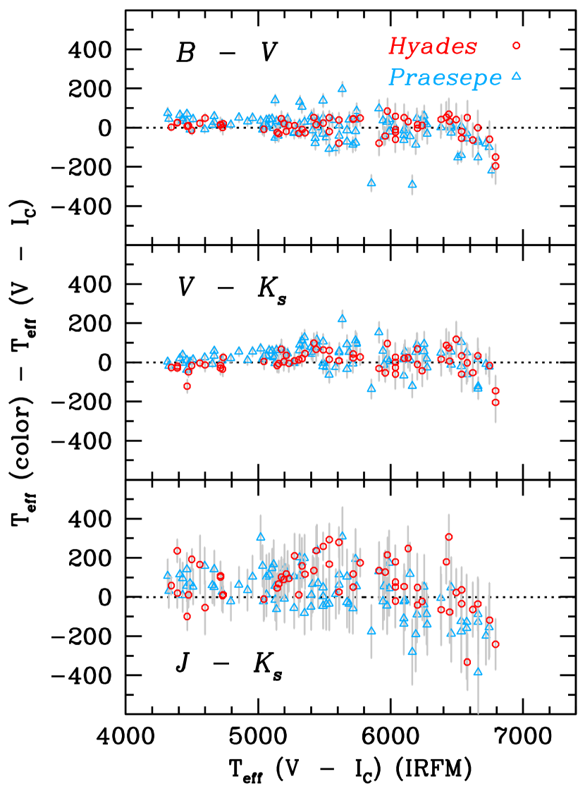
Figure 9.— Internal consistency of the IRFM $T_{\rm eff}$ estimates for the Hyades (red circles) and Praesepe stars (blue triangles). Comparisons are shown for each color index with respect to the $T_{\rm eff}$ values determined from $V\,-\,I_{C}$ at [Fe/H]$=0.13$ for the Hyades and [Fe/H]$=0.14$ for Praesepe. Error bars represent $\pm 1\sigma$ uncertainty propagated from photometric errors.

Figure 10.— Same as in Figure 9, but for the Pleiades at [Fe/H]$=0.04$. Note that low-mass Pleiades stars ($T_{\rm eff}\lesssim 5000$ K) are known to have anomalously blue colors in $B\,-\,V$. These stars could also have slight near-IR excesses, which may have affected $T_{\rm eff}$ values from $J\,-\,K_{s}$.

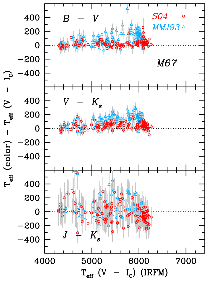
Figure 11.— Same as in Figure 9, but for M67 at [Fe/H]$=0.0$. Red circles and blue triangles represent comparisons based on the Sandquist (2004, S04) and Montgomery et al. (1993, MMJ93) photometry, respectively.

Figures 9–11 show how the IRFM $T_{\rm eff}$ determinations are internally consistent in the Jounson-Cousins-2MASS system in $B\,-\,V$, $V\,-\,I_{C}$, $V\,-\,K_{s}$, and $J\,-\,K_{s}$ using stars in four well-studied clusters: The Hyades (red circles in Figure 9), Praesepe (blue triangles in Figure 9), the Pleiades (Figure 10), and M67 (Figure 11). All of the stars shown in these figures are likely single-star members of each cluster after excluding known (unresolved) binaries. In Figure 11, we show results based on the two independent sets of M67 photometry from Montgomery et al. (1993, blue triangles) and Sandquist (2004, red circles). The compilation and individual sources of the cluster photometry can be found in An et al. (2007b).

To construct Figures 9–11 we corrected observed magnitudes for extinction using $E(V\,-\,I_{C})/E(B\,-\,V)=1.26$, $E(V\,-\,K_{s})/E(B\,-\,V)=2.82$, and $E(J\,-\,K_{s})/E(B\,-\,V)=0.53$ (An et al., 2007a). Foreground reddening values of $E(B\,-\,V)=0.000\pm 0.002$, $0.006\pm 0.002$, $0.032\pm 0.003$, and $0.041\pm 0.004$ mag were used for the Hyades, Praesepe, the Pleiades, and M67 respectively (An et al., 2007b). The IRFM $T_{\rm eff}$ equations in C10 include metallicity terms, and we adopted [Fe/H]$=+0.13\pm 0.01$, $+0.14\pm 0.02$, $+0.04\pm 0.02$, and $+0.00\pm 0.01$ dex for the Hyades, Praesepe, the Pleiades, and M67, respectively, based on high-resolution spectroscopic abundance analysis (see references in An et al., 2007b). Only the $(B\,-\,V)$-based estimates are significantly impacted by metallicity corrections, and the relative abundance differences in these well-studied open clusters are unlikely to be substantial enough to affect our results.

Table 5Statistical Properties of Clusters Comparisons

	$\Delta T_{\rm eff}$ (K)
Cluster Data	$4000<T_{\rm eff}\leq 7400$	$4000<T_{\rm eff}\leq 6000$	$6000<T_{\rm eff}\leq 7400$	$\sigma_{\rm sys}$
T${}_{\rm eff}(B\,-\,V,{\rm IRFM})-$ T${}_{\rm eff}(V\,-\,I_{C},{\rm IRFM})$
Hyades	$10.3\pm 6.7$	$11.5\pm 6.0$	$-2.9\pm 15.3$	$4.0$
Praesepe	$11.3\pm 7.4$	$23.0\pm 7.4$	$-59.4\pm 15.3$	$6.7$
Pleiades	$54.3\pm 12.1$	$67.5\pm 13.3$	$-5.5\pm 19.0$	$6.5$
M67 (MMJ93)	$74.1\pm 7.9$	$71.5\pm 8.5$	$93.2\pm 21.0$	$4.3$
M67 (S04)	$28.8\pm 4.0$	$16.7\pm 4.2$	$36.1\pm 7.7$	$5.3$
T${}_{\rm eff}(V\,-\,K_{s},{\rm IRFM})-$ T${}_{\rm eff}(V\,-\,I_{C},{\rm IRFM})$
Hyades	$-3.8\pm 7.4$	$-4.0\pm 7.6$	$-1.9\pm 16.7$	$0.9$
Praesepe	$23.2\pm 6.2$	$25.0\pm 6.7$	$1.6\pm 13.7$	$1.0$
Pleiades	$10.8\pm 5.9$	$9.0\pm 6.9$	$19.2\pm 13.9$	$1.1$
M67 (MMJ93)	$87.3\pm 7.7$	$81.8\pm 8.7$	$133.8\pm 19.6$	$0.5$
M67 (S04)	$34.1\pm 3.9$	$36.7\pm 4.9$	$29.9\pm 6.2$	$1.2$
T${}_{\rm eff}(J\,-\,K_{s},{\rm IRFM})-$ T${}_{\rm eff}(V\,-\,I_{C},{\rm IRFM})$
Hyades	$94.7\pm 17.0$	$108.3\pm 15.7$	$36.0\pm 32.9$	$3.9$
Praesepe	$44.2\pm 13.1$	$66.2\pm 13.7$	$-97.8\pm 34.8$	$4.0$
Pleiades	$-10.1\pm 13.9$	$-0.6\pm 14.8$	$-55.3\pm 30.7$	$5.4$
M67 (MMJ93)	$51.8\pm 16.6$	$61.4\pm 18.3$	$9.1\pm 38.6$	$6.3$
M67 (S04)	$-47.3\pm 14.1$	$-18.7\pm 18.5$	$-86.7\pm 21.7$	$7.3$
T${}_{\rm eff}(V\,-\,I_{C},{\rm IRFM})-$ T${}_{\rm eff}(M_{V},{\rm YREC})$
Hyades	$-12.1\pm 8.7$	$-8.3\pm 8.3$	$-56.4\pm 15.4$	$6.4$
Praesepe	$-14.7\pm 6.6$	$-12.2\pm 7.4$	$-52.9\pm 11.9$	$21.3$
Pleiades	$-14.6\pm 8.4$	$-9.9\pm 8.4$	$-50.5\pm 20.3$	$13.9$
M67 (MMJ93)	$-52.9\pm 8.6$	$-34.4\pm 7.5$	$-178.4\pm 13.7$	$22.0$
M67 (S04)	$-20.4\pm 3.4$	$-13.5\pm 3.5$	$-37.1\pm 8.2$	$24.1$
T${}_{\rm eff}(J\,-\,K_{s},{\rm IRFM})-$ T${}_{\rm eff}(M_{V},{\rm YREC})$
Hyades	$62.2\pm 16.6$	$90.9\pm 12.5$	$-35.1\pm 32.5$	$6.9$
Praesepe	$7.9\pm 14.9$	$43.9\pm 13.0$	$-152.5\pm 27.5$	$17.5$
Pleiades	$1.2\pm 15.9$	$22.6\pm 17.6$	$-92.8\pm 26.9$	$11.4$
M67 (MMJ93)	$-50.1\pm 15.9$	$-16.5\pm 19.2$	$-123.8\pm 28.4$	$35.3$
M67 (S04)	$-60.1\pm 15.8$	$-31.9\pm 18.8$	$-127.7\pm 29.1$	$30.4$

The $\pm 1\sigma$ error bars in Figures 9–11 are those propagated from the photometric errors only. Mean differences in the IRFM $T_{\rm eff}$ and the errors in the mean are provided in Table 5. Global differences are shown for stars at $4000<T_{\rm eff}\leq 7400$ K, and those cooler and hotter than $6000$ K are shown in the table. The $\sigma_{\rm sys}$ represents a total systematic error in this comparison from the reddening and metallicity errors (summed in quadrature); however, systematic errors are less important than random errors because of the precise E$(B\,-\,V)$ and [Fe/H] estimates of these well-studied clusters.

The low-mass stars in the Pleiades are known to have anomalously blue colors related to stellar activity in these heavily spotted, rapidly rotating, young stars (Stauffer et al., 2003). The temperature anomaly for $B\,-\,V$ at $T_{\rm eff}\lesssim 5000$ K in Figure 10, which is $\sim 200$ K larger than that for more massive stars, reflects this known effect and therefore is not a proper test of internal consistency in old field stars (such as those in the KIC). The M67 data may also be inappropriate for the test of the IRFM internal consistency, but with a different reason. Two independent photometry sets lead to a different conclusion: Montgomery et al. (1993) photometry shows internally less consistent IRFM $T_{\rm eff}$ for M67 stars than Sandquist (2004). A similar argument was made in An et al. (2007b), based on the differential metallicity sensitivities of stellar isochrones in different color indices (see Figure $11$ in the above paper); see also VandenBerg et al. (2010) for an independent confirmation of the systematic zero-point issue with the Montgomery et al. (1993) photometry.

Our cluster tests based on the Hyades and Praesepe demonstrate the internal consistency of the C10 color-$T_{\rm eff}$ relations in $B\,-\,V$, $V\,-\,I_{C}$, and $V\,-\,K_{s}$. The mean differences in $T_{\rm eff}$ among these color indices are typically few tens of degrees for both hot and cool stars (Table 5). Some of these mean differences could be systematic in nature, but they are generally consistent with the scatter in the C10 IRFM calibrations. However, the $(J\,-\,K_{s})-T_{\rm eff}$ relation tends to produce hotter $T_{\rm eff}$ than those from other color indices for these cluster stars (see bottom panel in Figure 9). The mean differences between $T_{\rm eff}(V\,-\,I_{C})$ and $T_{\rm eff}(J\,-\,K_{s})$ are $95$ K and $44$ K for the Hyades and Praesepe, respectively. There is also a hint of the downturn in the comparison for the hot stars in these clusters, where $(J\,-\,K_{s})-T_{\rm eff}$ produces cooler temperatures than $(V\,-\,I_{C})-T_{\rm eff}$ relation. The $\sim 100$ K offset between the hot and the cool stars roughly defines the size of the systematic error in the IRFM technique of C10 in $J\,-\,K_{s}$.

The Pleiades stars show a weaker systematic $T_{\rm eff}$ trend for the cool and the hot stars than the Hyades and Praesepe. In spite of this good agreement, we caution that this could be a lucky coincidence because the Pleiades low-mass stars probably have slight near-IR excesses in $K_{s}$ (Stauffer et al., 2003). The main-sequence turn-off of M67 is relatively cool, so the difference is only suggestive.

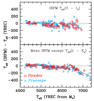
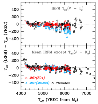
Figure 12.— Left: The $T_{\rm eff}$ comparisons between IRFM and YREC for stars in the Hyades (red circles) and Praesepe (blue triangles). Right: Same as in the left panels, but for the Pleiades stars (black circles), M67 stars from Sandquist (2004, red circles) photometry and from that of Montgomery et al. (1993, blue triangles). Top: IRFM $T_{\rm eff}$ from $V\,-\,I_{C}$. Bottom: Mean IRFM $T_{\rm eff}$ from $B\,-\,V$, $V\,-\,I_{C}$, and $V\,-\,K_{s}$. The YREC $T_{\rm eff}$ was estimated from the luminosity ($M_{V}$) of each star. Black line in the bottom left panel shows a moving averaged trend of the $T_{\rm eff}$ difference.

Figure 12 shows comparisons between the IRFM and YREC $T_{\rm eff}$ estimates. The left panel shows the comparisons for the Hyades and Praesepe stars, while the right panel shows those for the Pleiades and M67 stars. The IRFM $T_{\rm eff}$ on top panels was computed based on the $(V\,-\,I_{C})-T_{\rm eff}$ relation in C10, just as those used for a principal $T_{\rm eff}$ estimator in the above comparisons (Figures 9–11). The YREC $T_{\rm eff}$ was estimated using An et al. (2007b) isochrones, which have the same underlying set of interior models as those used in the current analysis. The model $T_{\rm eff}$ was computed at a constant $M_{V}$ of individual stars, assuming $(m\,-\,M)_{0}=3.33\pm 0.01$, $6.33\pm 0.04$, $5.63\pm 0.02$, and $9.61\pm 0.03$ mag for the distance moduli of the Hyades ($550$ Myr), Praesepe ($550$ Myr), the Pleiades ($100$ Myr), and M67 ($3.5$ Gyr), respectively (see references in An et al., 2007b).

Table 5 lists weighted mean differences between YREC and IRFM $T_{\rm eff}$. The mean difference between the $(V\,-\,I_{C})$-based IRFM and the luminosity-based YREC $T_{\rm eff}$ for cool stars ($T_{\rm eff}<6000$ K) is less than $20$ K, but the differences rise above $6000$ K to the $50$ K level. The difference between the $(J\,-\,K_{s})$-based IRFM and $M_{V}$-based YREC $T_{\rm eff}$ shows different offsets for the cool and hot stars; this trend is consistent with the above comparison between $(J\,-\,K_{s})$-based IRFM and other IRFM determination.

The bottom panel in Figure 12 shows comparisons between the YREC $T_{\rm eff}$ and the average IRFM $T_{\rm eff}$ from $B\,-\,V$, $V\,-\,I_{C}$, and $V\,-\,K_{s}$. Our results using $J\,-\,K_{s}$ as a thermometer are consistent with our earlier finding in Section 3.1 that C10 $(J\,-\,K_{s})$-based $T_{\rm eff}$ values are systematically cooler than those from the $griz$-based YREC models for hot stars (above about $6000$ K). The $(J\,-\,K_{s})$-based $T_{\rm eff}$ differ both from other IRFM diagnostics and the values inferred from SDSS colors for cooler stars, while the mean values inferred from the IRFM are close to SDSS for the cooler stars.

We therefore conclude that the cool star temperature scales are consistent, while there is evidence for a systematic departure at the hot end. A similar pattern emerges when we compare with spectroscopy, as discussed in the next section. Caution is therefore required in assigning errors for stars with formal temperature estimates above $6000$ K.

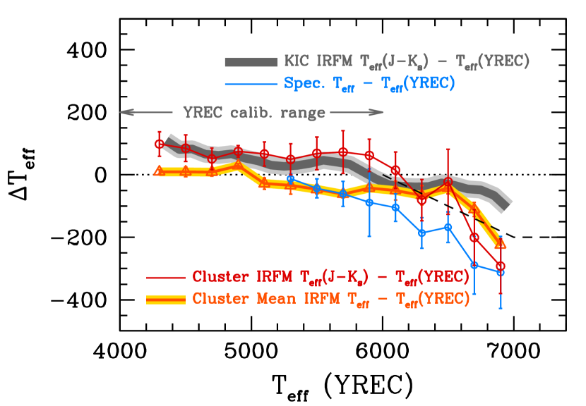
Figure 13.— Systematic differences of various $T_{\rm eff}$ estimates with respect to the YREC scale. Grey line shows the mean trend for the main KIC sample discussed in this work. The red line represents the difference with the $(J\,-\,K_{s})$-based IRFM $T_{\rm eff}$ for the open cluster sample (Hyades and Praesepe), while the orange line shows that with respect to the mean IRFM values from $B\,-\,V$, $V\,-\,I_{C}$, $V\,-\,K_{s}$. The blue line shows the trend for the B11 spectroscopic sample. Error bars in all cases represent $\pm 1\sigma$ error in the mean difference. Our adopted hot-$T_{\rm eff}$ corrections are shown with a black dashed line. Note that the empirical color-$T_{\rm eff}$ corrections in YREC are defined at $4000\leq T_{\rm eff}\leq 6000$ K in SDSS colors.

Systematic $T_{\rm eff}$ differences are shown in Figure 13. The red line represents the difference with the $(J\,-\,K_{s})$-based IRFM $T_{\rm eff}$ for the open cluster sample (Hyades and Praesepe), while the orange line shows that with respect to the mean IRFM values from $B\,-\,V$, $V\,-\,I_{C}$, $V\,-\,K_{s}$. Error bars indicate $\pm 1\sigma$ error in the mean difference. The difference between the average IRFM scale and the SDSS scale in the clusters is less than $25$ K on average from $4000$–$6000$ K, which we take as a conservative systematic temperature uncertainty in that domain. The differences are moderately larger for the IRFM $J\,-\,K_{s}$ temperature alone, but that diagnostic is also different from other IRFM thermometers for cool stars.

The differences in the hot cluster stars reflect actual differences in the calibrations, not issues peculiar to the photometry, extinction, or blending. We therefore attribute the comparable differences seen in the KIC stars (gray band) as caused by calibration issues in $J\,-\,K_{s}$ rather than as a reflection of systematics between the IRFM and SDSS systems. Furthermore, the SDSS calibration was based on M67 data, where the hotter turnoff stars ($T_{\rm eff}>6000$ K) were saturated. As a result, we believe that an adjustment closer to the IRFM scale is better justified.

A simple correction term, of the form below

$$T_{\rm eff,SDSS}<6000~{}K : T_{\rm eff,corr}=T_{\rm eff}{\rm(SDSS)},$$ (6)

$$6000~{}K\leq T_{\rm eff,SDSS}<7000~{}K :$$ (7)

$$T_{\rm eff,corr}=0.8\ (T_{\rm eff}{\rm(SDSS)} - 6000~{}K)+6000~{}K,$$ (8)

$$T_{\rm eff,SDSS}\geq 7000~{}K:T_{\rm eff,corr} = T_{\rm eff}{\rm(SDSS)}-200~{}K$$ (9)

brings the two scales into close agreement across their mutual range of validity. This empirical correction is indicated by the black dashed line in Figure 13. Below we find offsets similar in magnitude and opposite in sign between the IRFM and spectroscopic temperatures for hotter stars. Although this does not necessarily indicate problems with the fundamental scales, it does imply that systematic temperature scale differences are important for these stars.

3.4. Comparison with Spectroscopy

Spectroscopy provides a powerful external check on the precision of photometric temperature estimates. Spectroscopic temperatures are independent of extinction, and can be less sensitive to unresolved binary companions and crowding. In this section we therefore compare the photometric and spectroscopic temperature estimates for two well-studied samples in the Kepler fields. Bruntt et al. (2011, hereafter B11) reported results for $93$ stars with asteroseismic data, including 83 stars in our sample. Molenda-Żakowicz et al. (2011, hereafter MZ11) reported results for $78$ stars, including $45$ targets in common with our sample. The MZ11 data for cool stars are mostly subgiants and giants, while the bulk of the dwarf sample is hotter than $6000$ K. The B11 sample is similarly distributed, with the transition from the cool evolved to the hot unevolved sample occurring at $5500$ K.

All comparisons below are for the corrected photometric scale, adjusted for concordance with the IRFM at the hot end. We compare spectroscopic methods both with the fixed-metallicity ([Fe/H]$=-0.2$) temperatures in the catalog and the refined temperature estimates made possible with the addition of metallicity information and theoretical metallicity corrections. We excluded outliers in the following statistical comparisons using a $3\sigma$ outlier rejection.

As demonstrated below, we find that the two spectroscopic samples have different zero-points with respect to both the SDSS and KIC samples, indicating the importance of systematic errors in such comparisons. The photometric scale for the cool dwarfs and giants are in good agreement with the B11 scale, while both are offset relative to MZ11. The situation is different for hot dwarfs. The IRFM scale was cooler than the uncorrected SDSS scale. The spectroscopic samples are cooler than both. We interpret this as evidence of additional systematic uncertainties for the F stars, and discuss possible causes.

The stellar parameters for the MZ11 sample were derived using the Molenda-Żakowicz et al. (2007) template approach. The spectra were compared with a library of reference stars. The surface gravity, effective temperature, and metallicity were derived from a weighted average of the five closest spectral matches in the catalog. B11 used asteroseismic surface gravities and derived effective temperatures from traditional Boltzmann-Saha consistency arguments.

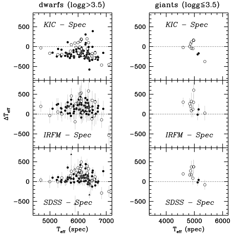
Figure 14.— Comparisons of spectroscopic $T_{\rm eff}$ with KIC (top), IRFM from $J\,-\,K_{s}$ (middle), and SDSS estimates from $griz$ (bottom). Filled and open points are from Bruntt et al. (2011) and Molenda-Żakowicz et al. (2011), respectively. Left panels show dwarf comparisons (KIC $\log{g}>3.5$), while the right panels show giant comparisons (KIC $\log{g}\leq 3.5$). Triangles in the bottom two panels represent stars flagged as having internally inconsistent effective temperature estimates (see text).

We compare the spectroscopic and photometric temperature estimates in Figure 14. The top, middle, and bottom panels compare spectroscopic temperatures to those of the KIC, IRFM ($J\,-\,K_{s}$), and SDSS, respectively. Left panels show comparisons for dwarfs (KIC $\log{g}>3.5$), while the right panels show those for giants (KIC $\log{g}\leq 3.5$). Filled circles are the B11 data, while open circles are the MZ11 data. In total, $83$ out of $93$ sample stars in B11 were used in this comparison; the remaining $10$ stars do not have $griz$ photometry in all passbands, so were not included in our KIC subsample. For the same reason, we initially included 45 spectroscopic targets from MZ11, but later excluded 8 more stars with $g\,-\,r<0.1$ or $g\,-\,r>1.0$. Triangles in the bottom two panels represent stars flagged as having internally inconsistent effective temperature estimates (Section 4.2.4). Error bars show the expected random errors, with a $70$ K error adopted in the temperature for the individual B11 sample stars.

In the above comparisons, we corrected the IRFM temperature estimates for the spectroscopic metallicity measurement of each sample, although the $T_{\rm eff}$ corrections in C10 were negligible ($\Delta T_{\rm eff}\approx 18$ K) in $J\,-\,K_{s}$. We also used individual stellar isochrones at each spectroscopic metallicity to estimate SDSS $T_{\rm eff}$ from $griz$, assuming a constant age of $1$ Gyr at all metallicity bins. However, the net effect of these corrections was small ($\Delta T_{\rm eff}\approx 25$ K), because $griz$-$T_{\rm eff}$ relations are relatively insensitive to metallicity and the mean metallicities of the spectroscopic samples are close to our fiducial value ($\langle{\rm[Fe/H]}\rangle=-0.07\pm 0.02$ and $-0.11\pm 0.03$ for the B11 and MZ11 samples, respectively). The SDSS $T_{\rm eff}$ values for giants were corrected for the $\log{g}$ difference from the dwarf temperature scale as described in Section 3.2.

Both spectroscopic samples for dwarfs are systematically hotter than the KIC (top left panel in Figure 14). The weighted average difference between the B11 sample and the KIC, in the sense of the KIC minus spectroscopic values, is $-170$ K with a dispersion of $116$ K, after a $3\sigma$ outlier rejection. The MZ11 sample is closer to the KIC, with a $-82$ K mean difference and a dispersion of $172$ K. This difference of $88$ K is a reflection of the systematic errors in the spectroscopic temperature scales. In the above comparisons, we did not include stars with inconsistent SDSS temperature measurements (triangles in Figure 14).

The weighted average difference between the B11 sample and the SDSS (in the sense SDSS $-$ Spec) for dwarfs is $85$ K with a $95$ K dispersion, after excluding those flagged as having discrepant $T_{\rm eff}$(YREC) values. If the metallicity corrections to the SDSS values were not taken into account (i.e., based on models at [Fe/H]$=-0.2$), the mean difference becomes $73$ K, but the dispersion increases to $111$ K.

However, there is a strong temperature dependence in the offset. Below $6000$ K the mean difference is $50$ K with a dispersion of $47$ K. For the hotter stars the mean difference is $101$ K with a dispersion of $118$ K. The blue line in Figure 13 shows a moving averaged difference between the B11 spectroscopic values and SDSS $T_{\rm eff}$ without the hot-end $T_{\rm eff}$ corrections (equations 6–8).

Although the size of the dwarf sample in MZ11 is small, it is found that the effective temperatures are systematically cooler than the SDSS values, with a weighted mean offset of $152$ K (SDSS $-$ Spec) and a dispersion of $175$ K. The difference is temperature dependent, being $53$ K for the stars below $6000$ K and $178$ K above it. These differences are $3$ K and $77$ K larger, respectively, than the results from the B11 sample. The temperature differences between photometry and spectroscopy are therefore smaller than the differences between the spectroscopic measurements and the KIC, while there is a real difference at the hot end even when systematic differences between the two spectroscopic samples are accounted for.

The B11 sample includes only two giants (KIC $\log{g}\leq 3.5$), but their spectroscopic temperatures are consistent with both IRFM and SDSS temperatures (see middle and bottom right panels in Figure 14). On the other hand, the MZ11 sample shows a large offset from IRFM ($\Delta T_{\rm eff}=245$ K) and SDSS ($\Delta T_{\rm eff}=206$ K), while the KIC and the MZ11 values agree with each other ($\Delta T_{\rm eff}=9$ K).

The cool MZ11 stars are mostly subgiants and giants, while the B11 cool sample includes a large dwarf population between $5000$ K and $6000$ K. The difference between the two cool end results - good agreement with B11 for cool dwarfs, but not with MZ11 - is real. This could reflect systematic differences between the dwarf and corrected giant results for the SDSS or the templates adopted by MZ11 for the evolved and unevolved stars. The scatter between the MZ11 results and the photometric ones is substantially larger than that between B11 and photometric temperature estimates. It would be worth investigating the zero-point of the templates used in the former method, as well as the random errors, in light of the results reported here.

In the section above we have focused on differences between the scales; it is fair to ask how both might compare to the true temperatures. The photometric scale is at heart simply an empirical relationship between color and the definition of the effective temperature itself ($L=4\pi R^{2}\sigma T_{\rm eff}^{4}$), and therefore the scale itself should be sound where the photometric relations are well-defined. However, the photometric methods can fail if there is more than one contributor to the photometry, or if the reddening is incorrectly measured. Spectroscopic temperatures measure physical conditions in the atmosphere, and are only indirectly tied to the fundamental flux per unit area, which defines the effective temperature. There are also systematic uncertainties between different methods for inferring effective temperatures, for example, fitting the wings of strong lines, or the use of Boltzmann-Saha solutions based on ionization and excitation balance. Finally, both photometric and spectroscopic estimates are only as good as their assumptions; stars with large surface temperature differences will be poorly modeled by both methods.

Our primary conclusion is therefore that the various dwarf temperature methods, spectroscopic and photometric, are in good agreement for the cooler stars. Systematic effects are at or below the 50 K level. The hotter stars in the sample have real systematic differences between spectroscopic and photometric temperatures, and similar discrepancies are also present between the photometric methods themselves. This is further evidence that work is needed to tie down more precisely the temperature scale above $6000$ K, and that larger systematic errors should be assigned in this domain until such an analysis is performed. We have less data for the giants, but there does appear to be a real difference between the photometric results and the temperatures inferred for the MZ11 sample.

3.5. Effects of Binaries on Colors

Unresolved binaries in the sample could bias a color-based $T_{\rm eff}$ estimate. Unless the mass ratio of the primary and secondary components in the binary system is close to either unity (twins) or zero (negligible contributions from the secondary), composite colors of the system are redder than those from the primaries alone, leading towards systematically lower $T_{\rm eff}$. It is difficult to directly flag potential binaries given the filters available to us, and as a result we do not include star by star corrections in the table. However, such a systematic bias will be important when evaluating the bulk properties of the KIC sample. In this section, we therefore estimate the size of the bias due to unresolved binaries in the KIC, and provide statistical corrections for the effect of unresolved binary companions on average effective temperature estimates.

Binary contamination effects on the color-$T_{\rm eff}$ relations were derived by performing artificial star tests. We used a $1$ Gyr old Padova models at solar abundance (Girardi et al., 2004). These models include stellar masses down to $0.15\ M_{\odot}$, allowing us to include low-mass systems outside the formal range of the SDSS color calibration. The absolute color-$T_{\rm eff}$ relations in these models are not exactly the same as in our base calibration, and the adoption of a solar metallicity isochrone is not strictly self-consistent with our application of the base model at [Fe/H]$=-0.2$. However, our main purpose is to evaluate the relative temperature errors induced by companions, and the effects of these offsets are presumably small.

We assumed a $50\%$ binary fraction with $10,000$ single stars and $10,000$ binary systems. Primary masses were randomly drawn from a Salpeter mass function, while we explored three different choices for the relative masses of the secondaries: Salpeter, flat, and one drawn from the open cluster M35 (Barrado y Navascués et al., 2001). A flat mass function is expected for short-period binaries, which will be a minority of the sample; this is thus a limiting case. In the artificial star simulations, we derived empirical color-color sequences in $g\,-\,i$, $g\,-\,z$, and $J\,-\,K_{s}$ with $g\,-\,r$ as the principal color index. We simulated photometric errors by injecting dispersions of $0.01$ mag in $gri$, $0.03$ mag in $z$, $0.024$ mag in $J$, and $0.028$ mag in $K_{s}$. These 2MASS errors are median values of the actual photometric errors in the KIC sample.

Figure 15.— Average color bias in $g\,-\,i$, $g\,-\,z$, and $J\,-\,K_{s}$ at fixed $g\,-\,r$ due to unresolved binaries for three different assumptions about the secondary mass function. Points and error bars are the centroid and the error in the mean distribution from the simulations. A $50\%$ binary fraction is assumed.

The result of these binary simulations is presented in Figure 15, which shows the mean deviations in $g\,-\,i$, $g\,-\,z$, and $J\,-\,K_{s}$ from those with primaries alone. For Figure 15 we fitted a Gaussian for each $g\,-\,r$ bin to estimate the mean color offset and the uncertainty as shown by circles and error bars. The three curves indicate results from three different relative mass functions for secondaries.

Table 6Binary Corrections

				$\langle\Delta T_{\rm eff}\rangle$
$g\,-\,r$	$\Delta(g\,-\,i)$	$\Delta(g\,-\,z)$	$\Delta(J\,-\,K_{s})$	$g\,-\,r$	$g\,-\,i$	$g\,-\,z$	$J\,-\,K_{s}$
(mag)	(mag)	(mag)	(mag)	(K)	(K)	(K)	(K)
M35 Mass Function
$0.25$	$0.001$	$0.000$	$0.006$	$18$	$21$	$23$	$83$
$0.35$	$0.000$	$0.002$	$0.012$	$25$	$28$	$32$	$89$
$0.45$	$0.002$	$0.004$	$0.010$	$27$	$32$	$35$	$70$
$0.55$	$0.004$	$0.006$	$0.010$	$31$	$38$	$43$	$77$
$0.65$	$0.002$	$0.007$	$0.009$	$32$	$36$	$42$	$93$
$0.75$	$0.002$	$0.010$	$0.014$	$30$	$34$	$40$	$121$
$0.85$	$0.002$	$0.012$	$0.008$	$25$	$31$	$37$	$97$
$0.95$	$0.004$	$0.014$	$0.011$	$22$	$29$	$35$	$71$
$1.05$	$0.006$	$0.014$	$0.007$	$18$	$26$	$31$	$35$
Flat Mass Function
$0.25$	$0.002$	$0.002$	$0.008$	$34$	$38$	$42$	$98$
$0.35$	$0.001$	$0.003$	$0.011$	$40$	$43$	$48$	$106$
$0.45$	$0.001$	$0.004$	$0.012$	$42$	$45$	$51$	$104$
$0.55$	$0.003$	$0.006$	$0.012$	$45$	$51$	$56$	$93$
$0.65$	$0.002$	$0.006$	$0.011$	$44$	$48$	$53$	$115$
$0.75$	$0.001$	$0.009$	$0.011$	$39$	$42$	$50$	$129$
$0.85$	$0.002$	$0.010$	$0.009$	$34$	$39$	$45$	$104$
$0.95$	$0.002$	$0.011$	$0.015$	$28$	$33$	$39$	$91$
$1.05$	$0.006$	$0.016$	$0.013$	$21$	$30$	$35$	$54$
Salpeter Mass Function
$0.25$	$0.001$	$0.002$	$0.004$	$7$	$9$	$10$	$50$
$0.35$	$0.000$	$0.002$	$0.004$	$11$	$12$	$15$	$49$
$0.45$	$0.001$	$0.005$	$0.008$	$12$	$15$	$18$	$43$
$0.55$	$0.002$	$0.005$	$0.007$	$12$	$16$	$19$	$43$
$0.65$	$0.003$	$0.007$	$0.012$	$13$	$18$	$22$	$78$
$0.75$	$0.003$	$0.010$	$0.007$	$13$	$18$	$24$	$73$
$0.85$	$0.003$	$0.011$	$0.009$	$11$	$17$	$23$	$74$
$0.95$	$0.004$	$0.013$	$0.007$	$10$	$17$	$23$	$51$
$1.05$	$0.007$	$0.014$	$0.009$	$10$	$18$	$23$	$21$

Note. — The sense of the bias is that populations mixed with unresolved binaries look redder (cooler) at a given $g\,-\,r$ in the above color indices.

The sizes of these color shifts are shown in Table 6. The systematic color shift due to unresolved binaries is less strongly dependent on the choice of secondary mass functions. Typical sizes of these color shifts are $\sim 0.003$ mag, $0.008$ mag, and $0.010$ mag in $g\,-\,i$, and $g\,-\,z$, and $J\,-\,K_{s}$, respectively. To correct for the unresolved binaries in the KIC, the above color shifts should be subtracted before estimating $T_{\rm eff}$. The last four columns in Table 6 list the average $T_{\rm eff}$ difference between a population with a $50\%$ unresolved binary fraction and that of primaries alone. The sense is that unresolved binary stars have lower temperatures than expected from primaries alone. Different SDSS color indices have similar binary sensitivities, and temperatures based on these filters are less affected by unrecognized companions than those derived using $J\,-\,K_{s}$. These color shifts are small for any given star, but significant when applied to the entire catalog. We therefore recommend including them when using large samples of photometric effective temperature estimates, and include this effect in our global error budget below.

3.6. Other Sources of Uncertainties and Error Budget

We can assess our overall errors by comparing the real to the observed dispersions in the color-color plane. Photometric errors, unresolved binaries, and metallicity all induce scatter; so would extinction uncertainties. Significant mismatches between the two reflect unrecognized or overestimated error sources.

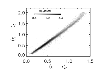
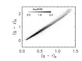
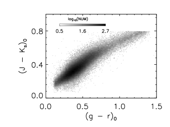
Figure 16.— Extinction corrected color-color relations in the KIC, after the zero-point corrections as described in Section 2.2. Only those with $\log{g}>3.5$ are shown.

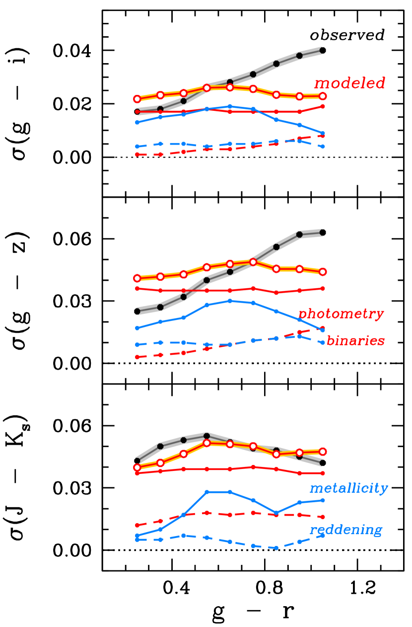
Figure 17.— Comparison between observed (thick black line with closed circles) and modeled (thick red line with open circles) dispersions of the color-color sequence as a function of $g\,-\,r$. The modeled dispersion is a quadrature sum of individual error contributions: photometric errors (red solid), unresolved binaries (red dashed), metallicity (blue solid), and reddening (blue dashed).

Figure 16 shows the observed color-color diagrams in the KIC, after the extinction corrections and the zero-point adjustment as described in Section 2.2. From Figure 16, we estimated the standard deviation of the color dispersion from a fiducial line (fit using a $5^{th}$ order polynomial) in $g\,-\,i$, $g\,-\,z$, and $J\,-\,K_{s}$ at each $g\,-\,r$ bin. These observed dispersions with good $T_{\rm eff}$ estimates are shown as solid black curves with closed circles in Figure 17. Here the criteria for the good $T_{\rm eff}$ are that the standard deviation of individual $T_{\rm eff}$ from three color indices ($g\,-\,r$, $g\,-\,i$, and $g\,-\,z$) is less than $130$ K or that the difference between SDSS and IRFM measurements is no larger than three times the random errors of these measurements (see also Section 4.2.4). There is a strong overlap between the two criteria. Since the formal random SDSS errors are of order $40$ K, and the systematics between the colors are typically at that level as well, differences of $130$ K represent clear evidence of a breakdown in the color-temperature relationships, likely from unresolved blends. Excluding extreme outliers is essential because they would otherwise dominate the dispersion measure, and we are interested in testing the properties of the majority of the sample.

Other lines in Figure 17 represent contributions from random photometric errors, unresolved binaries or photometric blends, metallicity, and dust extinction as described below. Red lines with open circles are the quadrature sum of all of these error sources.

We assumed $0.01$ mag errors in $gri$, $0.03$ mag errors in $z$, $0.024$ mag in $J$, and $0.028$ mag in $K_{s}$ to estimate color dispersions from photometric errors alone (red curve in Figure 17). To perform this simulation in $grizJK_{s}$, we combined our base model (Table 1) with our earlier set of isochrones in the 2MASS system (An et al., 2007b) at the same metallicity ([Fe/H]$=-0.2$) and age ($1$ Gyr) as those for the base isochrone. As with the binary simulations described in the previous section, we employed a $1$ Gyr old, solar metallicity Padova model (Girardi et al., 2004) to generate color-color sequences with a $50\%$ binary fraction based on the M35 mass function for secondaries. Again, running this isochrone in the simulation is not strictly consistent with the usage of our base model, but the relative effects induced by unresolved companions would be rather insensitive to the small metallicity difference. The dispersion induced by unresolved binaries is shown in a red dashed curve in Figure 17.

The KIC sample has a mean [Fe/H]$=-0.2$ with a standard deviation of $0.28$ dex. If the KIC [Fe/H] values are accurate enough for these stars, this metallicity spread would induce a significant spread in $T_{\rm eff}$. The color dispersion due to metal abundances was estimated by taking the color difference between our base model ([Fe/H]$=-0.2$) and the models at [Fe/H]$=+0.1$ and $-0.5$ as an effective $\pm 1\sigma$ uncertainty. The metallicity error contribution is shown in blue solid curves. The KIC sample has a wide range of reddening values ($0\lesssim E(B\,-\,V)\lesssim 0.2$). We took $0.02$ mag error as an approximate $\pm 1\sigma$ error in E$(B\,-\,V)$, roughly equivalent to a 15 % fractional uncertainty for a typical star. Stars on the simulated color-color sequence were randomly displaced from their original positions assuming this E$(B\,-\,V)$ dispersion. The resulting color dispersion is shown with the blue dashed curves in Figure 17.

In Figure 17 there is a color-dependent trend in the error budget, where observed color dispersion increases for cooler stars in $g\,-\,i$ and $g\,-\,z$. On the other hand, the simulated dispersions (open circles connected with solid red curves) are essentially flat. Our results are consistent with expectations in $J\,-\,K$; if anything, the random errors appear to be overstated. This is probably caused by correlated errors in $J$ and $K_{s}$, which were treated as uncorrelated in the temperature error estimates.

Based on this exercise, we conclude that our error model is reasonable for the hot stars in the sample, especially when the stars most impacted by blends are removed. There is excess color scatter for red stars, which correspond to effective temperatures below $\sim 5000$ K in our sample. About $16\%$ of the sample are found in this temperature domain. This could reflect contamination of the dwarf sample by giants, which have different color-color relationships; or a breakdown in the photometric error model for red stars. It would be useful to revisit this question when we have a solid estimate of the giant contamination fraction for the cool dwarfs in the sample.

4. The Revised $T_{\rm eff}$ Catalog

4.1. A Recipe for Estimating $T_{\rm eff}$

We present results for the long-cadence sample with the overall properties of the catalog and systematic error estimates in this section. We have not provided corrected values for the entire KIC, because the additional quality control is outside the scope of our effort. However, our method could be applied in general to the KIC, employing the following steps.

Table 7Catalog with Revised $T_{\rm eff}$

	SDSS				IRFM				KIC
KIC ID	$T_{\rm eff}$	$\sigma_{\rm tot}$	$\sigma_{\rm ran}$		$T_{\rm eff}$	$\sigma_{\rm tot}$	$\sigma_{\rm ran}$		$T_{\rm eff}$	$\log{g}$	[Fe/H]	$\Delta T_{\rm eff}$	flag
	(K)	(K)	(K)		(K)	(K)	(K)		(K)	(dex)	(dex)	(K)
757076	$5137$	$85$	$55$		$5150$	$98$	$94$		$5174$	$3.60$	$-0.08$	$0$	$0$
757099	$5523$	$97$	$34$		$5270$	$110$	$101$		$5589$	$3.82$	$-0.21$	$0$	$0$
757137	$4822$	$74$	$42$		$4536$	$101$	$99$		$4879$	$2.58$	$-0.08$	$49$	$0$
757218	$4728$	$79$	$17$		$4489$	$90$	$75$		$4555$	$2.28$	$-0.12$	$67$	$0$
757231	$4909$	$116$	$64$		$4974$	$111$	$89$		$4825$	$2.60$	$-0.08$	$24$	$0$

Note. — Only a portion of this table is shown here to demonstrate its form and content. A machine-readable version of the full table is available.

Note. — Effective temperatures presented here were computed at a fixed [Fe/H]$=-0.2$.

• Correct the KIC $griz$ photometry onto the SDSS DR8 system using equations 1–4.

• Apply the KIC extinctions and the extinction coefficients in Section 2 to obtain dereddened colors.

• Use our $griz$-$T_{\rm eff}$ polynomials (Table 2) or the original isochrone (Table 1) to obtain temperature estimates. If complementary IRFM estimates are desired, use the C10 polynomials (for $V_{T}JK_{s}$).

• Adjust hot-end temperatures above $6000$ K using equations 5–7. The polynomials in Table 2 are for the original SDSS temperature calibration (Table 1) without the hot-end adjustment described in Section 3.3.

• In Table 7 we adopted a metallicity [Fe/H]$=-0.2$ and a dispersion of $0.3$ dex for error purposes. We also adopted a fractional error of $15\%$ in the extinction.

• The SDSS temperatures are inferred from the weighted average of the independent color estimates using the photometric errors discussed in Section 2, and the random uncertainties are the maximum of the formal random errors and the dispersion in those inferred from different $griz$ colors.

• If the metallicity is known independent of the KIC, the SDSS temperatures can be corrected using the values in Table 3 and if desired the IRFM temperatures can be corrected for metallicity by adopting star-by-star metallicities in the C10 formulae.

• Apply gravity corrections in Table 4 for giants with $\log{g}{\rm(KIC)}\leq 3.5$.

• Outside the temperature range of the SDSS calibration, zero-point shifts of $223$ K at the hot end and $150$ K at the cool end should be applied to the KIC $T_{\rm eff}$ to avoid artificial discontinuities in the temperature scale at the edges of validity of the method.

• In our revised $T_{\rm eff}$ table, we did not apply statistical corrections for binaries, but the current Table 6 could be employed to do so, and this should be included in population studies.

• We expect about $4\%$ of the sample to have photometry impacted by blends. Such stars could be identified as those having an excess dispersion from individual SDSS colors on the order of $130$ K or more, and/or as those showing more than a $3\sigma$ deviation from the mean difference between the IRFM and SDSS temperatures.

4.2. Main $T_{\rm eff}$ Catalog

Our main result, the revised $T_{\rm eff}$ for $161,977$ stars in the long-cadence KIC, is presented in Table 7. All of our revised $T_{\rm eff}$ estimates in the catalog are based on the recalibrated $griz$ magnitudes in the KIC (Section 2.2). In addition to the $griz$-based SDSS $T_{\rm eff}$, Table 7 contains $(J\,-\,K_{s})$-based IRFM $T_{\rm eff}$ using the original C10 relation, and KIC values along with $\log{g}$ and [Fe/H] in the KIC. The null values in the SDSS $T_{\rm eff}$ column are those outside of the color range in the model ($4043$ K $<T_{\rm eff}<7509$ K). Similarly, the C10 IRFM $T_{\rm eff}$ are defined at $0.07\leq(J\,-\,K_{s})_{0}\leq 0.80$.

Table 8Statistical Properties of $T_{\rm eff}$

$\langle T_{\rm eff}\rangle$			IRFM $-$ KIC				SDSS $-$ KIC				SDSS $-$ IRFM				$T_{\rm eff}$(color) $-$ $T_{\rm eff}$($griz$)				SDSS
(KIC)	$\langle(g\,-\,r)_{0}\rangle$	${\rm N_{stars}}$	$\Delta T_{\rm eff}$	$\sigma$	$\sigma_{\rm prop}$		$\Delta T_{\rm eff}$	$\sigma$	$\sigma_{\rm prop}$		$\Delta T_{\rm eff}$	$\sigma$	$\sigma_{\rm prop}$		$g\,-\,r$	$g\,-\,i$	$g\,-\,z$		$\sigma_{griz}$	$\sigma_{\rm prop}$
dwarfs (KIC $\log{g}>3.5$)
$6597$	$0.13$	$1032$	$165$	$182$	$184$		$223$	$41$	$46$		$54$	$172$	$191$		$-9$	$-2$	$14$		$33$	$43$
$6501$	$0.15$	$1480$	$167$	$172$	$180$		$224$	$36$	$46$		$50$	$170$	$188$		$-11$	$-1$	$13$		$33$	$43$
$6393$	$0.18$	$2156$	$180$	$182$	$184$		$228$	$35$	$46$		$40$	$176$	$191$		$-15$	$-2$	$19$		$34$	$42$
$6296$	$0.21$	$3029$	$190$	$185$	$188$		$231$	$34$	$46$		$34$	$181$	$195$		$-18$	$-2$	$23$		$36$	$41$
$6201$	$0.24$	$4239$	$211$	$183$	$186$		$237$	$32$	$45$		$23$	$181$	$194$		$-20$	$-1$	$24$		$37$	$40$
$6095$	$0.27$	$6551$	$209$	$193$	$195$		$242$	$30$	$45$		$32$	$195$	$202$		$-24$	$-1$	$28$		$39$	$39$
$5995$	$0.30$	$8154$	$203$	$199$	$197$		$250$	$30$	$45$		$42$	$201$	$205$		$-28$	$-1$	$29$		$41$	$37$
$5899$	$0.33$	$9685$	$220$	$192$	$194$		$258$	$31$	$45$		$34$	$197$	$202$		$-31$	$0$	$30$		$43$	$36$
$5802$	$0.36$	$11632$	$225$	$194$	$193$		$266$	$32$	$44$		$35$	$199$	$202$		$-36$	$1$	$31$		$44$	$36$
$5697$	$0.39$	$12398$	$235$	$191$	$192$		$265$	$42$	$45$		$20$	$201$	$201$		$-41$	$2$	$37$		$44$	$35$
$5596$	$0.43$	$11492$	$240$	$188$	$187$		$244$	$44$	$43$		$-6$	$200$	$196$		$-41$	$3$	$33$		$42$	$34$
$5502$	$0.46$	$9946$	$234$	$180$	$181$		$227$	$45$	$41$		$-20$	$194$	$190$		$-40$	$3$	$31$		$42$	$32$
$5400$	$0.49$	$8914$	$230$	$176$	$176$		$216$	$44$	$39$		$-26$	$189$	$184$		$-35$	$2$	$27$		$38$	$30$
$5302$	$0.53$	$7370$	$214$	$170$	$168$		$206$	$47$	$37$		$-23$	$183$	$176$		$-34$	$2$	$27$		$38$	$29$
$5201$	$0.57$	$6119$	$195$	$157$	$158$		$203$	$49$	$35$		$-9$	$173$	$166$		$-30$	$1$	$25$		$37$	$27$
$5099$	$0.60$	$6112$	$184$	$149$	$149$		$201$	$50$	$34$		$1$	$166$	$156$		$-26$	$1$	$25$		$36$	$25$
$5002$	$0.65$	$4619$	$177$	$134$	$140$		$192$	$53$	$32$		$-3$	$156$	$147$		$-29$	$1$	$26$		$36$	$22$
$4901$	$0.70$	$3587$	$180$	$129$	$135$		$187$	$54$	$30$		$-11$	$149$	$142$		$-24$	$1$	$26$		$35$	$20$
$4804$	$0.75$	$2829$	$178$	$122$	$131$		$177$	$59$	$29$		$-23$	$145$	$138$		$-22$	$0$	$26$		$34$	$18$
$4703$	$0.81$	$1887$	$179$	$120$	$128$		$162$	$57$	$26$		$-39$	$137$	$134$		$-16$	$0$	$25$		$31$	$16$
$4605$	$0.86$	$1384$	$182$	$123$	$126$		$161$	$61$	$23$		$-36$	$140$	$130$		$-7$	$-2$	$19$		$27$	$15$
$4498$	$0.91$	$809$	$201$	$118$	$123$		$174$	$52$	$20$		$-26$	$127$	$127$		$5$	$-4$	$11$		$23$	$14$
$4396$	$0.98$	$1258$	$223$	$115$	$118$		$179$	$41$	$18$		$-45$	$118$	$121$		$7$	$-4$	$9$		$20$	$13$
$4302$	$1.06$	$1421$	$237$	$109$	$110$		$176$	$34$	$17$		$-69$	$102$	$113$		$7$	$-3$	$11$		$18$	$12$
$4200$	$1.14$	$1157$	$257$	$97$	$104$		$169$	$28$	$16$		$-95$	$94$	$107$		$11$	$-3$	$10$		$16$	$11$
$4099$	$1.21$	$1022$	$279$	$74$	$97$		$150$	$19$	$17$		$-134$	$73$	$101$		$26$	$-3$	$10$		$19$	$11$
giants (KIC $\log{g}\leq 3.5$)
$5292$	$0.51$	$35$	$246$	$204$	$122$		$216$	$38$	$35$		$-62$	$198$	$132$		$-5$	$-4$	$29$		$34$	$29$
$5184$	$0.56$	$175$	$167$	$111$	$112$		$214$	$41$	$36$		$30$	$132$	$121$		$-30$	$-2$	$37$		$39$	$27$
$5086$	$0.60$	$676$	$159$	$100$	$108$		$216$	$43$	$34$		$38$	$102$	$117$		$-30$	$-1$	$33$		$37$	$25$
$4995$	$0.65$	$2098$	$135$	$99$	$105$		$215$	$42$	$33$		$58$	$105$	$114$		$-34$	$1$	$32$		$38$	$23$
$4897$	$0.69$	$3376$	$129$	$96$	$101$		$220$	$41$	$32$		$68$	$101$	$110$		$-33$	$2$	$29$		$37$	$21$
$4800$	$0.74$	$4316$	$124$	$91$	$98$		$225$	$40$	$30$		$76$	$96$	$105$		$-30$	$3$	$26$		$36$	$19$
$4702$	$0.79$	$3435$	$118$	$91$	$94$		$236$	$39$	$28$		$93$	$95$	$101$		$-26$	$4$	$22$		$34$	$17$
$4599$	$0.85$	$3002$	$110$	$95$	$91$		$254$	$35$	$23$		$124$	$100$	$96$		$-18$	$5$	$16$		$28$	$16$
$4509$	$0.91$	$1148$	$71$	$106$	$87$		$261$	$32$	$20$		$174$	$112$	$91$		$-12$	$5$	$11$		$23$	$14$
$4401$	$0.97$	$930$	$58$	$97$	$84$		$294$	$27$	$17$		$227$	$103$	$87$		$-3$	$4$	$3$		$18$	$13$
$4307$	$1.03$	$861$	$64$	$80$	$81$		$313$	$27$	$16$		$239$	$86$	$84$		$3$	$4$	$-2$		$16$	$12$
$4202$	$1.10$	$665$	$97$	$53$	$79$		$313$	$30$	$14$		$208$	$58$	$81$		$12$	$3$	$-5$		$13$	$12$
$4105$	$1.20$	$631$	$169$	$29$	$80$		$321$	$148$	$14$		$129$	$87$	$83$		$-64$	$98$	$-5$		$15$	$11$

Note. — Statistical properties derived from the full long-cadence sample, after applying the hot $T_{\rm eff}$ corrections. No metallicity and binary corrections were applied.

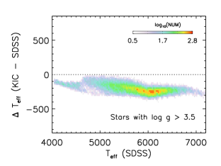
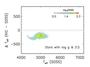
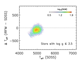
Figure 18.— Comparisons of $T_{\rm eff}$ using the final SDSS $T_{\rm eff}$ estimates. Comparisons are shown for the original KIC $T_{\rm eff}$ for dwarfs (top left) and giants (top right), and for the $(J\,-\,K_{s})$-based IRFM estimates for dwarfs (bottom left) and giants (bottom right).

Statistical properties of our final temperature estimates are listed in Table 8 for dwarfs and for giants, separately. The relative KIC, IRFM, and SDSS temperatures for dwarfs and giants in the final catalog are compared in Figure 18. These comparisons include the adjustment to the hot end published SDSS scale described in Section 3.3. We did not correct the IRFM temperature estimates for gravity effects in the giants. The discrepancy between the two scales for the cool giants is consistent with being caused by this effect, as can be seen from the gravity sensitivity of $(J\,-\,K_{s})$ in Figure 7.

Below we describe each column of Table 7, and provide a summary on how to correct $T_{\rm eff}$ for different $\log{g}$, binarity (blending), and metallicity.

4.2.1 Error Estimates in $T_{\rm eff}$

For the SDSS and IRFM, we estimated total ($\sigma_{\rm tot}$) and random ($\sigma_{\rm ran}$) errors for individual stars as follows. The random errors for the SDSS were taken from two approaches, tabulating whichever yields the larger value: a propagated error from the photometric precision and the one from measurements of $T_{\rm eff}$ from individual color indices ($g\,-\,r$, $g\,-\,i$, and $g\,-\,z$). For the former, we repeated our procedures of solving for $T_{\rm eff}$ with $0.01$ mag photometric errors in $gri$ and $0.03$ mag errors in $z$: we added corresponding $T_{\rm eff}$ errors from individual determinations. The random errors for the IRFM were estimated from the 2MASS-reported photometric errors in $J$ and $K_{s}$ (combined in quadrature).

In Table 7 we included systematic errors from $\pm 15\%$ error in the foreground dust extinction and $\pm 0.3$ dex error in [Fe/H] from our fiducial case ([Fe/H]$=-0.2$) for both SDSS and IRFM measurements. The total error ($\sigma_{\rm tot}$) is a quadrature sum of both random and systematic error components. The total errors are dominated by the extinction uncertainties, which relate to both galactic position and distance. The quoted values yield dispersions in temperature between YREC, IRFM, and spectroscopy consistent with the data. We present effective temperatures defined at a fixed [Fe/H]$=-0.2$. If it is desired to correct for metallicities different from this fiducial [Fe/H], $T_{\rm eff}$ corrections in Table 3 can be used.

4.2.2 Corrections for different $\log{g}$

Our application of the isochrone assumes that all of the stars are main-sequence dwarfs. To correct for differences between the KIC and the model $\log{g}$ values, we used $\log{g}$ sensitivities of the $griz$ colors using Castelli & Kurucz (2004) ATLAS9 models, as described in Section 3.2. Table 4 lists the correction factors in $T_{\rm eff}$ as a function of each color index over $\Delta\log{g}=0.5$–$3.0$ in a $0.5$ dex increment. For a given color in each of these color indices, a difference between the KIC and the model $\log{g}$ can be estimated ($\Delta\log{g}=\log{g}_{\rm KIC}\,-\,\log{g}_{\rm YREC}$), and the corresponding $\Delta T_{\rm eff}$ values in Table 4 can be found in $g\,-\,r$, $g\,-\,i$, and $g\,-\,z$, respectively. The mean $\Delta T_{\rm eff}$ correction was then added to the dwarf-based $T_{\rm eff}$ estimates. Our catalog (Table 7) lists SDSS $T_{\rm eff}$ estimates already corrected using these $\log{g}$ corrections for those with $\log{g}{\rm(KIC)}\leq 3.5$ at $T_{\rm eff}{\rm(SDSS)}<5300$ K. If it is desired to recover the dwarf-based solution, correction terms ($\Delta T_{\rm eff}$) in Table 7 should be subtracted from the listed $T_{\rm eff}{\rm(SDSS)}$.

4.2.3 Corrections for Binaries

As described in Section 3.5, unresolved binaries and blending can have an impact on the overall distribution of photometric $T_{\rm eff}$. If the population effect is of greater importance than individual $T_{\rm eff}$, correction factors in Table 6 should be added to the SDSS and IRFM $T_{\rm eff}$ (making them hotter) in Table 7. With $1\%-3\%$ errors in $griz$ photometry, it is difficult to distinguish between single stars with unresolved binaries and/or blended sources in the catalog.

4.2.4 Quality Control Flag

The last column in Table 7 shows a quality control flag. If the flag is set (${\tt flag}=1$), the SDSS $T_{\rm eff}$ values should be taken with care. The flag was set

• if the standard deviation of individual $T_{\rm eff}$ from three color indices ($g\,-\,r$, $g\,-\,i$, and $g\,-\,z$) exceeds $130$ K ($N=1,402$)

• or if the difference between SDSS and IRFM measurements is greater than $3\sigma$ random errors (summed in quadrature) with respect to the mean trend ($N=4,388$). Only those at $4700<T_{\rm eff}<7000$ K for dwarfs and $4700<T_{\rm eff}<5400$ K for giants were flagged this way, to avoid a biased $\Delta T_{\rm eff}$ distribution at the cool and hot temperature range (see Figure 18).

• or if any of the $griz$ measurements are not reported in the KIC ($N=257$).

In total, $5,798$ stars (about $4\%$ of $154,931$ stars with a valid SDSS $T_{\rm eff}$) were flagged this way.

4.3. IRFM $T_{\rm eff}$ from Tycho-2MASS System

Table 9Tycho-2MASS-based IRFM $T_{\rm eff}$

	$T_{\rm eff}(V_{T}-J)$				$T_{\rm eff}(V_{T}-H)$				$T_{\rm eff}(V_{T}-K_{s})$				$T_{\rm eff}(J-K_{s})$
KIC_ID	$T_{\rm eff}$	$\sigma_{\rm tot}$	$\sigma_{\rm ran}$		$T_{\rm eff}$	$\sigma_{\rm tot}$	$\sigma_{\rm ran}$		$T_{\rm eff}$	$\sigma_{\rm tot}$	$\sigma_{\rm ran}$		$T_{\rm eff}$	$\sigma_{\rm tot}$	$\sigma_{\rm ran}$
1026309	$4684$	$102$	$84$		$4607$	$90$	$72$		$4623$	$79$	$60$		$4469$	$103$	$96$
1160789	$4997$	$59$	$48$		$4915$	$47$	$37$		$4951$	$44$	$33$		$4866$	$122$	$120$
1717271	$4346$	$63$	$24$		$4279$	$65$	$27$		$4327$	$57$	$20$		$4267$	$105$	$95$
1718046	$4811$	$106$	$81$		$4708$	$86$	$62$		$4754$	$82$	$57$		$4625$	$112$	$105$
1718401	$\cdots$	$\cdots$	$\cdots$		$\cdots$	$\cdots$	$\cdots$		$\cdots$	$\cdots$	$\cdots$		$6531$	$164$	$161$

Note. — Only a portion of this table is shown here to demonstrate its form and content. A machine-readable version of the full table is available.

Note. — Effective temperatures presented here were computed at a fixed [Fe/H]$=-0.2$.

In addition to our main catalog in Table 7, we also present in Table 9 the IRFM $T_{\rm eff}$ in Tycho $V_{T}$ and 2MASS $JHK_{s}$ colors for $7,912$ stars. These stars are a subset of the long-cadence KIC sample, which are bright enough to have $V_{T}$ magnitudes, and can be used as an independent check on our $T_{\rm eff}$ scale (see lower left panel in Figure 6). The IRFM $T_{\rm eff}$ values are presented using $V_{T}\,-\,J$, $V_{T}\,-\,H$, $V_{T}\,-\,K_{s}$, and $J\,-\,K_{s}$, with both random $(\sigma_{\rm ran})$ and total $(\sigma_{\rm tot})$ errors. As in Table 7, random errors are propagated from photometric uncertainties, and total errors are a quadrature sum of random and systematic errors ($15\%$ error in reddening and $0.3$ dex error in [Fe/H]).

5. Summary and Future Directions

The Kepler mission has a rich variety of applications, all of which are aided by better knowledge of the fundamental stellar properties. We have focused on the effective temperature scale, which is a well-posed problem with the existing photometry. However, in addition to the revised KIC temperature there are two significant independent results from our investigation. We have identified a modest color-dependent offset between the KIC and SDSS DR8 photometry, whose origin should be investigated. Applying the relevant corrections to the KIC photometry significantly improves the internal consistency of temperature estimates. We have also verified that the independent temperature scales (Johnson-Cousins and SDSS) of An et al. and those from recent IRFM studies (Casagrande et al.) are in good agreement, permitting a cross-calibration of the latter to the SDSS filter system. Below we summarize our main results for the KIC, then turn to the major limitations of our main catalog, a brief discussion of the implications, and prospects for future improvements.

5.1. Summary

Our main result is a shift to higher effective temperatures than those included in the existing KIC. We have employed multiple diagnostic tools, including two distinct photometric scales and some high-resolution spectroscopy. In the case of cool (below $6000$ K) dwarfs, the various methods for assigning effective temperature have an encouraging degree of consistency. The Johnson-Cousins measurements of An et al. (2007a) are in good agreement with the independent IRFM temperatures from C10 in star clusters. In Table 5, for example, the $V\,-\,I_{c}$ results agree within 15 K for all clusters if we adopt the Sandquist (2004) dataset for M67. The SDSS-based A09 system is constructed to be on the same absolute scale as the An et al. (2007a) system, so a similar level of agreement is expected between the IRFM and the temperatures that we derive from the SDSS filters. A comparison of the IRFM and SDSS temperatures in the KIC confirms this pattern, with agreement to better than 100 K for the cool stars. Even this level of disagreement overestimates the underlying accord in the systems, because the IRFM ($J\,-\,K_{s}$) diagnostic that was available to us in the KIC has systematic offsets relative to other IRFM thermometers even in the open clusters. When we correct for these offsets, the agreement for cool stars between the SDSS-based method of A09 and the IRFM ($J\,-\,K_{s}$) temperatures is very good, with average differences below $25$ K and maximum differences below the $50$ K level. Our cool dwarf temperatures are also within $50$ K on average when compared to the spectroscopic results from B11. The spectroscopic sample of MZ11 is cooler at the $88$ K level, which we take as a measure of systematic uncertainties in the spectroscopic scale (See Bruntt et al., 2010, for a further comparison of the spectroscopic and fundamental temperature scales).

For hotter dwarfs the revised temperature estimates are higher than in the KIC, but the magnitude of the offset is not consistent between the two photometric scales and the spectroscopic data. Motivated by this offset, we adjusted the SDSS-based system of A09 to be cooler on average by 100 K between 6000 K and 7000 K on the IRFM system. The consistency between photometric and spectroscopic scales degrades for stars in this range. This could reflect defects in the fundamental temperature scale for hotter stars; the existing fundamental data for the IRFM include relatively few solar-abundance dwarfs above $6000$ K. There could also be errors in photometric or spectroscopic temperature estimates from the onset of rapid rotation above 6300 K, or color anomalies from chemically peculiar hot stars. On the spectroscopic side, it would be valuable to compare the atmospheric temperatures inferred from Boltzman and Saha constraints to fundamental ones; as discussed in C10, there can be significant systematic offsets between these scales for some systems. This issue deserves future scrutiny and additional fundamental data would be very helpful.

In the case of evolved stars we also found a hotter temperature scale than in the KIC. We had to employ theoretical estimates of gravity sensitivity, however, to temperature diagnostics derived for dwarfs. An extension of the fundamental work to giants has been performed for other colors in the past, and it would be beneficial to test the theoretical predictions against actual radius data.

5.2. Cautions and Caveats in Usage of the Catalog

There are some significant drawbacks of the existing catalog, and care is required in its proper application. Binary companions will modify the colors and temperatures of stars; we have provided tables for statistical corrections, but have not included this in the tabulated effective temperatures. Blending can also impact colors, and there is clear evidence of some blended objects in our comparison of the KIC to SDSS DR8 data with superior resolution. The major error source for the temperature estimates is the uncertainty in the extinction. We have adopted a global percentage value based on typical errors in extinction maps, but there could be larger local variations. The color combinations available to us have limited diagnostic power for star-by-star extinction and binary corrections. For population studies, the stars in the long-cadence KIC sample were selected for a planet transit survey, and do not represent an unbiased set of the underlying population.

The KIC abundance estimates have significant errors, largely because the filters with the greatest metallicity sensitivity were not available. As a result, we have adopted metallicity insensitive temperature diagnostics, but the temperatures should be corrected for individual metallicities if available. These effects are at the 100 K per dex level, and will therefore be smaller than the extinction uncertainties for most stars in the sample. The $\log{g}$ values for hot stars are not well-constrained in the KIC, but we have adopted KIC gravities for cool stars. Our results would be affected at a modest level by changes in the derived gravities, and the appropriate corrections should be made if precise values are available.

There are two open areas for further discussion as well: the appropriate temperature scale for the hot dwarfs and errors in the photometry. In the former case, we recommend adjustments above 6000 K to the SDSS scale. For the entire domain we also note inconsistencies between the $J\,-\,K_{s}$ calibration and the other color-temperature relationships in the IRFM. Even after putting the fundamental photometric temperature scale on a common system, however, there is a difference between it and the spectroscopic scale for stars above $6000$ K. Until it is resolved we recommend inclusion of systematic temperature errors in this domain. The impact of the $\log{g}$ determinations on the extinction estimates for the hot stars should be investigated as well. The gravity diagnostics for the hot stars are not well measured, and asteroseismic gravities confirm this expected lack of precision. The KIC catalog included this as an ingredient in the distance estimates, but it is difficult to reconstruct the weights and importance of this uncertainty after the fact. Star-by-star extinctions would be useful for this purpose.

The origin of the differences between the SDSS (DR8) and KIC photometry should also be tracked down, and there may be spatially dependent or magnitude dependent terms. We also noted some cases with severe internal inconsistency in the photometric temperature diagnostics, and flagged those which we identified. We believe that unresolved blends are a promising candidate, but further work on this front is warranted. In a small fraction of cases these photometric issues can cause severe errors in the temperatures. Effective temperatures for stars where different colors return very different estimates should be treated with caution.

Despite these reservations, we believe that the addition of temperatures more closely tied to the fundamental scale will significantly improve the reliability of inferences about the underlying stellar populations.

5.3. Implications and Future Directions

A shift to higher effective temperatures will have consequences for both planetary and stellar science. On the main sequence, hotter stars will be on average more massive and larger. This would imply larger planet radii on average for such objects. The radii of evolved stars require more information (especially from surface gravity effects), and the consequences of the temperature scale shift for them are more difficult to predict from first principles. Stars of known asteroseismic radius will be on average more luminous, which could partially explain discrepancies in the mass-radius relationship for evolved stars (Chaplin et al., 2011). Asteroseismic parameters defined with scaling relationships will also be impacted. A more precise absolute effective temperature scale will also permit more stringent constraints on asteroseismic properties from detailed modeling of the frequency spectrum (see Metcalfe et al., 2010).

However, the full potential will be realized as complementary information becomes available on the Kepler sample. Blue data (such as Johnson $UB$ or SDSS $u$) could be employed to infer more reliable photometric metallicities; Johnson-Cousins $UBV(RI)_{C}$ data would enable more reliable extinction estimates, binary discrimination, and broader application of the IRFM directly to stars in the sample. Photometric systems naturally designed for F-type stars, such as Strömgren, would be useful for addressing the temperature and surface gravity scales in that regime.

A more robust set of input data would provide an important control sample for the measured planet population; it will be challenging to obtain spectroscopic temperatures of both the planet candidates and the background stellar population. A better calibration of the fundamental temperature scale is possible once asteroseismic radii are combined with parallaxes in the Kepler field, either via Kepler data or through the Gaia mission. The time domain data from the satellite are exquisite; a proper application of complementary tools from stellar astrophysics is now essential to fully realize their considerable scientific promise.

Appendix A Erratum: “A Revised Effective Temperature Scale for the Kepler Input Catalog” (2012, ApJS, 199, 30)

A.1. Sign Errors in the Gravity Corrections

We derived surface gravity corrections to the color-temperature relationships for red giants. This step was required because we adopted a dwarf-based color calibration, and the theoretical correction is given in Figure 8. However, the sign of the correction was reversed in the note at the bottom of Table 4. In Table 7 the sense in which the corrections should have been applied is noted correctly, but the actual corrections used were reversed. In addition, null values ($-999$) in the gravity correction table were accidentally included in the interpolation by the sign flip error, which resulted in unreasonably large correction terms at the very cool end ($T_{\rm eff}\lesssim 4200$ K).

We have revised the data in Tables 4 and 7 accordingly, and updated the figures (Figures 8 and 18) and statistical properties (Table 8) that were impacted. Gravity terms were applied for stars with low gravities ($\log{g}\leq 3.5$), to correct for differences between the the Kepler Input Catalog (KIC) and the model $\log{g}$ values. The $T_{\rm eff}$ estimates for dwarfs with $\log{g}>3.5$ remain valid in the original version of Table $7$.

A revised version of the gravity corrections is found in Table 4, with the same form and content as in the original table, except its signs. Here, $\log{g}{\rm(YREC)}$ is the $\log{g}$ in our YREC model ($3^{\rm rd}$ column in Table 4). Negative values in the table mean that giants have lower $T_{\rm eff}$ than dwarfs at fixed colors. Therefore, $\Delta T_{\rm eff}$ values in Table 4 should be added to dwarf-based $T_{\rm eff}$ estimates, if one wishes to infer $T_{\rm eff}$ for giants or subgiants.

We also revised our scheme to handle the gravity corrections in the very cool end ($T_{\rm eff}\lesssim 4200$ K). A revised plot of the gravity corrections is presented in Figure 8. In this revision, a simple quadratic relation was used to extend theoretical $T_{\rm eff}$ corrections beyond theoretical computations, in a way that the correction terms become zero at $T_{\rm eff}\sim 4000$ K (see Figure $7$, where dwarf color-$T_{\rm eff}$ relations cross giant relations at $T_{\rm eff}\sim 4000$ K). However, only a minor fraction of stars in our sample ($\sim 400$ giants) are affected by this change.

A revised main catalog (Table 7) shows SDSS $T_{\rm eff}$ estimates, after correcting for the difference in gravity, at $\log{g}{\rm(KIC)}\leq 3.5$. For giants, the mean and median changes from the original version are $59$ K and $36$ K, respectively, at $T_{\rm eff}>4200$ K. The dwarf-based solution can be obtained by subtracting the tabulated correction terms ($\Delta T_{\rm eff}$) in Table 7.

Figure 18 is a replacement for the original figure, and shows comparisons of our revised $T_{\rm eff}$ with those of the KIC (top panels) and Infrared Flux Method (IRFM; bottom panels). Comparisons for dwarfs in the left panels are unaffected by the sign flips in the gravity corrections. However, an improved agreement is seen between the IRFM and SDSS (YREC) scales for red giants (lower right panel). The discrepancy with the original KIC remains, but the differences for cool giants are significantly smaller.

The corrected statistical properties of the temperature differences between SDSS, IRFM, and KIC estimates are shown in Table 8, a replacement for the original table. For hotter giants the differences from prior results are zero, while the magnitude of the error rises to $210$ K at the cool end of the calibration range. The weighted mean differences for giants are $-165$ K (a median difference of $-161$ K) for the KIC minus SDSS temperatures and $-47$ K (a median difference of $-42$ K) for the IRFM minus SDSS temperatures. The differences were $-252$ K (median $-215$ K) and $-109$ K (median $-92$ K), respectively, from prior results. A significant offset between the KIC and SDSS values remains, which is one of our main results in the paper.

The main focus of the original paper concerned the $T_{\rm eff}$ scale for dwarfs, which is not impacted. With the revised $\log{g}$ corrections, a smaller number of stars ($5,347$ versus $5,798$ among $154,931$ stars with a valid SDSS $T_{\rm eff}$) are now flagged as having internally inconsistent $T_{\rm eff}$ estimates, according to our quality criteria (Section 4.2.4). Comparisons of the revised $T_{\rm eff}$ for giants with spectroscopic samples in Figure 14 are unaffected, as the gravity corrections have correctly been applied in this case.

A.2. Detailed Steps to Compute Mean $T_{\rm eff}$ and its Errors

Regardless of the sign flip errors in the gravity corrections, we provide below detailed descriptions on how to obtain mean $T_{\rm eff}$ and its random and systematic errors using YREC isochrones in $griz$ passbands.

The mean $T_{\rm eff}$ can be determined in the following way. This compliments a description in the third step of “A Recipe for Estimating $T_{\rm eff}$” in Section 4.1 of the original paper. For a given set of $griz$ magnitudes, which were corrected for the photometry zero-point errors and interstellar extinctions in the previous steps, one can determine a mean distance modulus for each star using model magnitudes in $griz$:

$$(m\,-\,M)_{0}=\frac{\Sigma_{i}[(m_{{\rm obs},i}-m_{{\rm model},i})/\sigma^{2}_{i}]}{\Sigma_{i}(1/\sigma^{2}_{i})},$$ (A1)

where the subscript $i$ indicates each of the $griz$ passbands. The $m_{{\rm obs},i}$ and $\sigma_{i}$ are observed magnitude and its error ($0.01$ mag in $gri$ and $0.03$ mag in $z$) in each passband. The $m_{{\rm model},i}$ is the model magnitude in each passband from our base isochrone in Table $1$.

From this, one can compute a $\chi^{2}$ value of the model fit for each star as follows:

$$\chi^{2}=\Sigma_{i}\frac{[(m_{{\rm obs},i}-m_{{\rm model},i})-(m\,-\,M)_{0}]^{2}}{\sigma^{2}_{i}}.$$ (A2)

We searched for a minimum $\chi^{2}$ of the model fit in the entire mass grid of our base isochrone, and determined a mean $T_{\rm eff}$ as the one that gives the most consistent fit overall to the data in $griz$ passbands. The best-fitting $T_{\rm eff}$ is shown in the second column in Table 7.

Random errors in $T_{\rm eff}$ were obtained in the following way. We applied photometric errors to each passband ($\pm 0.01$ mag in $gri$ and $\pm 0.03$ mag in $z$), and computed $T_{\rm eff}$. Taking the mean difference from the original $T_{\rm eff}$ as an effective $1\sigma$ error, we added in quadrature $T_{\rm eff}$ errors from all photometric passbands in $griz$. We also computed a random error by taking a standard deviation of individual $T_{\rm eff}$ estimates from $g\,-\,r$, $g\,-\,i$, and $g\,-\,z$, respectively. We then took a larger one from the above two approaches as the size of a representative random source of error. This error is shown in the fourth column ($\sigma_{\rm ran}$) in Table 7.

Systematic errors in $T_{\rm eff}$ were estimated as follows. For the error in the reddening, we repeated computing $T_{\rm eff}$ with $15\%$ lower and higher $E(B\,-\,V)$ values than in the KIC, and took the mean difference from the original $T_{\rm eff}$ as an effective $\pm 1\sigma$ error. For the error from the metallicity, we computed $T_{\rm eff}$ from models at [Fe/H]$=-0.5$ and [Fe/H]$=+0.1$ (one can use our tabulated metallicity corrections in Table $3$), and took the mean difference from an original $T_{\rm eff}$ as an effective $\pm 1\sigma$ error in $T_{\rm eff}$. From both errors in reddening and metallicity, we obtained a total systematic error in $T_{\rm eff}$ by adding individual errors in quadrature. Based on both random and systematic errors, the total error was computed as a quadrature sum of these errors, and is tabulated in the $3^{\rm rd}$ column ($\sigma_{\rm tot}$) in Table 7.

Table 4Gravity Corrections

		$\log{g}$	$\log{g}{\rm(star)}-\log{g}{\rm(YREC)}$
$g-r$	$g-i$/$g-z$	(YREC)	$-0.5$	$-1.0$	$-1.5$	$-2.0$	$-2.5$	$-3.0$
$\Delta T_{\rm eff}$ when $T_{\rm eff}$ are estimated from $g-r$
$0.500$	$\cdots$	$4.57$	$0.0$	$0.0$	$0.0$	$0.0$	$0.0$	$0.0$
$0.550$	$\cdots$	$4.59$	$0.0$	$0.0$	$0.0$	$0.0$	$0.0$	$0.0$
$0.600$	$\cdots$	$4.61$	$-1.5$	$-2.2$	$-2.3$	$-2.0$	$-1.2$	$0.2$
$0.650$	$\cdots$	$4.62$	$-5.8$	$-8.1$	$-7.3$	$-4.5$	$0.2$	$7.2$
$0.700$	$\cdots$	$4.63$	$-11.2$	$-15.3$	$-12.9$	$-6.1$	$4.4$	$18.5$
$0.750$	$\cdots$	$4.64$	$-18.4$	$-26.6$	$-24.5$	$-13.8$	$3.8$	$25.7$
$0.800$	$\cdots$	$4.65$	$-28.2$	$-43.2$	$-44.3$	$-31.6$	$-7.3$	$22.8$
$0.850$	$\cdots$	$4.65$	$-36.2$	$-58.6$	$-65.1$	$-55.1$	$-29.0$	$6.6$
$0.900$	$\cdots$	$4.66$	$-41.2$	$-69.3$	$-81.0$	$-76.3$	$-54.2$	$-18.9$
$0.950$	$\cdots$	$4.66$	$-44.6$	$-77.2$	$-93.6$	$-94.7$	$-78.4$	$-45.1$
$1.000$	$\cdots$	$4.67$	$-47.1$	$-83.4$	$-103.8$	$-109.3$	$-97.9$	$-69.8$
$1.050$	$\cdots$	$4.67$	$-50.6$	$-88.9$	$-110.8$	$-118.8$	$-111.4$	$-88.2$
$1.100$	$\cdots$	$4.68$	$-51.5$	$-90.4$	$-111.8$	$-119.4$	$-114.0$	$-95.5$
$1.150$	$\cdots$	$4.69$	$-53.1$	$-90.2$	$-106.5$	$-109.9$	$-104.2$	$-88.6$
$1.200$	$\cdots$	$4.69$	$-48.4$	$-80.0$	$-87.8$	$-83.8$	$-75.8$	$-61.8$
$1.250$	$\cdots$	$4.70$	$-38.4$	$-56.8$	$-55.0$	$-44.8$	$-32.7$	$-18.7$
$1.300$	$\cdots$	$4.72$	$-17.5$	$-25.9$	$-21.6$	$-13.0$	$-2.7$	$7.8$
$1.350$	$\cdots$	$4.73$	$0.0$	$0.0$	$0.0$	$0.0$	$0.0$	$0.0$
$\Delta T_{\rm eff}$ from $g-i$
$0.500$	$0.655$	$4.57$	$0.0$	$0.0$	$0.0$	$0.0$	$0.0$	$0.0$
$0.550$	$0.725$	$4.59$	$0.0$	$0.0$	$0.0$	$0.0$	$0.0$	$0.0$
$0.600$	$0.795$	$4.61$	$-1.2$	$-1.8$	$-1.8$	$-1.4$	$-0.6$	$0.5$
$0.650$	$0.865$	$4.62$	$-5.2$	$-7.5$	$-6.5$	$-4.0$	$0.2$	$5.9$
$0.700$	$0.934$	$4.63$	$-10.3$	$-14.6$	$-13.3$	$-8.3$	$0.3$	$12.0$
$0.750$	$1.003$	$4.64$	$-16.9$	$-25.2$	$-25.8$	$-19.4$	$-7.0$	$10.3$
$0.800$	$1.071$	$4.65$	$-24.7$	$-38.7$	$-43.5$	$-37.4$	$-22.5$	$-0.9$
$0.850$	$1.138$	$4.65$	$-31.1$	$-50.8$	$-60.1$	$-57.1$	$-43.4$	$-21.5$
$0.900$	$1.205$	$4.66$	$-34.9$	$-58.6$	$-71.4$	$-72.3$	$-61.9$	$-42.8$
$0.950$	$1.272$	$4.66$	$-37.9$	$-65.1$	$-80.7$	$-85.2$	$-78.6$	$-63.0$
$1.000$	$1.341$	$4.67$	$-41.3$	$-70.9$	$-88.3$	$-95.3$	$-92.0$	$-79.2$
$1.050$	$1.411$	$4.67$	$-43.4$	$-74.3$	$-92.5$	$-101.1$	$-100.6$	$-90.4$
$1.100$	$1.483$	$4.68$	$-43.8$	$-75.3$	$-93.6$	$-102.7$	$-103.9$	$-95.9$
$1.150$	$1.559$	$4.69$	$-43.1$	$-73.7$	$-90.8$	$-98.7$	$-100.4$	$-94.2$
$1.200$	$1.639$	$4.69$	$-38.3$	$-66.2$	$-80.6$	$-85.9$	$-86.7$	$-82.0$
$1.250$	$1.724$	$4.70$	$-29.8$	$-52.7$	$-63.0$	$-63.2$	$-62.4$	$-58.5$
$1.300$	$1.816$	$4.72$	$-16.1$	$-31.1$	$-38.2$	$-34.7$	$-34.0$	$-30.9$
$1.350$	$1.920$	$4.73$	$-2.6$	$-6.0$	$-7.6$	$-6.1$	$-6.0$	$-5.2$
$\Delta T_{\rm eff}$ from $g-z$
$0.500$	$0.708$	$4.57$	$0.0$	$0.0$	$0.0$	$0.0$	$0.0$	$0.0$
$0.550$	$0.795$	$4.59$	$0.0$	$0.0$	$0.0$	$0.0$	$0.0$	$0.0$
$0.600$	$0.881$	$4.61$	$-0.8$	$-1.2$	$-1.1$	$-0.9$	$-0.4$	$0.4$
$0.650$	$0.966$	$4.62$	$-3.6$	$-5.1$	$-4.4$	$-2.5$	$0.3$	$4.4$
$0.700$	$1.050$	$4.63$	$-7.7$	$-11.2$	$-10.1$	$-6.3$	$-0.6$	$7.5$
$0.750$	$1.133$	$4.64$	$-13.5$	$-20.6$	$-20.7$	$-15.6$	$-7.5$	$4.2$
$0.800$	$1.215$	$4.65$	$-20.4$	$-32.5$	$-35.5$	$-30.7$	$-21.1$	$-6.5$
$0.850$	$1.294$	$4.65$	$-25.5$	$-41.7$	$-48.3$	$-46.4$	$-37.3$	$-22.4$
$0.900$	$1.373$	$4.66$	$-28.1$	$-47.0$	$-56.6$	$-58.3$	$-50.9$	$-37.5$
$0.950$	$1.452$	$4.66$	$-30.2$	$-51.6$	$-63.9$	$-68.4$	$-63.3$	$-51.8$
$1.000$	$1.533$	$4.67$	$-33.0$	$-56.5$	$-70.5$	$-76.7$	$-74.0$	$-64.3$
$1.050$	$1.616$	$4.67$	$-34.8$	$-59.9$	$-74.9$	$-82.2$	$-81.7$	$-73.9$
$1.100$	$1.703$	$4.68$	$-35.4$	$-61.3$	$-76.7$	$-84.6$	$-85.9$	$-80.0$
$1.150$	$1.794$	$4.69$	$-34.6$	$-60.1$	$-75.3$	$-83.2$	$-85.5$	$-81.3$
$1.200$	$1.891$	$4.69$	$-30.3$	$-53.7$	$-67.8$	$-74.9$	$-77.6$	$-75.2$
$1.250$	$1.995$	$4.70$	$-22.7$	$-42.1$	$-54.2$	$-59.5$	$-61.8$	$-61.0$
$1.300$	$2.110$	$4.72$	$-13.0$	$-25.9$	$-32.0$	$-40.3$	$-42.2$	$-41.6$
$1.350$	$2.241$	$4.73$	$-2.6$	$-5.3$	$-6.1$	$-8.9$	$-9.3$	$-9.2$

Note. — In the original version of Table 4, gravity corrections had sign flip errors. $\Delta T_{\rm eff}$ values in Table 4 should be added to dwarf-based $T_{\rm eff}$ estimates, if one wishes to infer $T_{\rm eff}$ for giants or subgiants.

Table 7Catalog with Revised $T_{\rm eff}$

	SDSS				IRFM				KIC
KIC_ID	$T_{\rm eff}$	$\sigma_{\rm tot}$	$\sigma_{\rm ran}$		$T_{\rm eff}$	$\sigma_{\rm tot}$	$\sigma_{\rm ran}$		$T_{\rm eff}$	$\log{g}$	[Fe/H]	$\Delta T_{\rm eff}$	Flag
	(K)	(K)	(K)		(K)	(K)	(K)		(K)	(dex)	(dex)	(K)
757076	$5137$	$85$	$55$		$5150$	$98$	$94$		$5174$	$3.60$	$-0.08$	$0$	$0$
757099	$5523$	$97$	$34$		$5270$	$110$	$101$		$5589$	$3.82$	$-0.21$	$0$	$0$
757137	$4724$	$74$	$42$		$4536$	$101$	$99$		$4879$	$2.58$	$-0.08$	$-49$	$0$
757218	$4594$	$79$	$17$		$4489$	$90$	$75$		$4555$	$2.28$	$-0.12$	$-67$	$0$
757231	$4861$	$116$	$64$		$4974$	$111$	$89$		$4825$	$2.60$	$-0.08$	$-24$	$0$

Note. — Only a portion of this table is shown here to demonstrate its form and content. A machine-readable version of the full table is available. In the original version of Table 7, there were sign flip errors in the gravity corrections ($\Delta T_{\rm eff}$), which affect SDSS $T_{\rm eff}$ for giants ($\log{g}\leq 3.5$) in the above table. Other columns are unaffected. Effective temperatures presented here were computed at a fixed [Fe/H]$=-0.2$.

Table 8Statistical Properties of $T_{\rm eff}$

$\langle T_{\rm eff}\rangle$			IRFM $-$ KIC				SDSS $-$ KIC				SDSS $-$ IRFM				$T_{\rm eff}$(color) $-$ $T_{\rm eff}$($griz$)				SDSS
(KIC)	$\langle(g\,-\,r)_{0}\rangle$	${\rm N_{stars}}$	$\Delta T_{\rm eff}$	$\sigma$	$\sigma_{\rm prop}$		$\Delta T_{\rm eff}$	$\sigma$	$\sigma_{\rm prop}$		$\Delta T_{\rm eff}$	$\sigma$	$\sigma_{\rm prop}$		$g\,-\,r$	$g\,-\,i$	$g\,-\,z$		$\sigma_{griz}$	$\sigma_{\rm prop}$
giants (KIC $\log{g}\leq 3.5$)
$5292$	$0.51$	$35$	$246$	$204$	$122$		$216$	$38$	$35$		$-62$	$198$	$132$		$-5$	$-4$	$29$		$34$	$29$
$5184$	$0.56$	$175$	$167$	$111$	$112$		$214$	$41$	$35$		$30$	$132$	$121$		$-31$	$-1$	$37$		$39$	$27$
$5086$	$0.60$	$676$	$159$	$100$	$108$		$215$	$45$	$34$		$36$	$104$	$117$		$-32$	$0$	$35$		$37$	$25$
$4995$	$0.65$	$2098$	$135$	$99$	$105$		$208$	$45$	$33$		$50$	$106$	$113$		$-38$	$1$	$36$		$38$	$23$
$4897$	$0.69$	$3376$	$129$	$96$	$101$		$207$	$44$	$32$		$52$	$103$	$110$		$-38$	$1$	$35$		$37$	$21$
$4800$	$0.74$	$4316$	$124$	$91$	$98$		$202$	$46$	$30$		$48$	$99$	$105$		$-38$	$1$	$36$		$36$	$19$
$4702$	$0.79$	$3435$	$118$	$91$	$94$		$192$	$51$	$27$		$39$	$101$	$101$		$-37$	$0$	$37$		$34$	$17$
$4599$	$0.85$	$3002$	$110$	$95$	$91$		$178$	$56$	$24$		$36$	$108$	$96$		$-30$	$-2$	$34$		$28$	$16$
$4509$	$0.91$	$1148$	$71$	$106$	$87$		$151$	$53$	$20$		$56$	$118$	$91$		$-25$	$-3$	$32$		$23$	$14$
$4401$	$0.97$	$930$	$58$	$97$	$84$		$148$	$46$	$17$		$75$	$109$	$87$		$-19$	$-5$	$29$		$18$	$13$
$4307$	$1.03$	$861$	$64$	$80$	$81$		$138$	$41$	$16$		$62$	$88$	$84$		$-16$	$-6$	$27$		$16$	$12$
$4202$	$1.10$	$665$	$97$	$53$	$79$		$123$	$32$	$14$		$20$	$60$	$81$		$-3$	$-7$	$19$		$13$	$12$
$4105$	$1.20$	$631$	$169$	$29$	$80$		$103$	$28$	$14$		$-60$	$33$	$83$		$22$	$-7$	$3$		$15$	$11$

Note. — We only present statistical properties for giants (KIC $\log{g}\leq 3.5$) in the revised Table 8. Results are the same for dwarfs (KIC $\log{g}>3.5$) in the original Table 8. Statistical properties derived from the full long-cadence sample, after applying the hot $T_{\rm eff}$ corrections. No metallicity and binary corrections were applied.

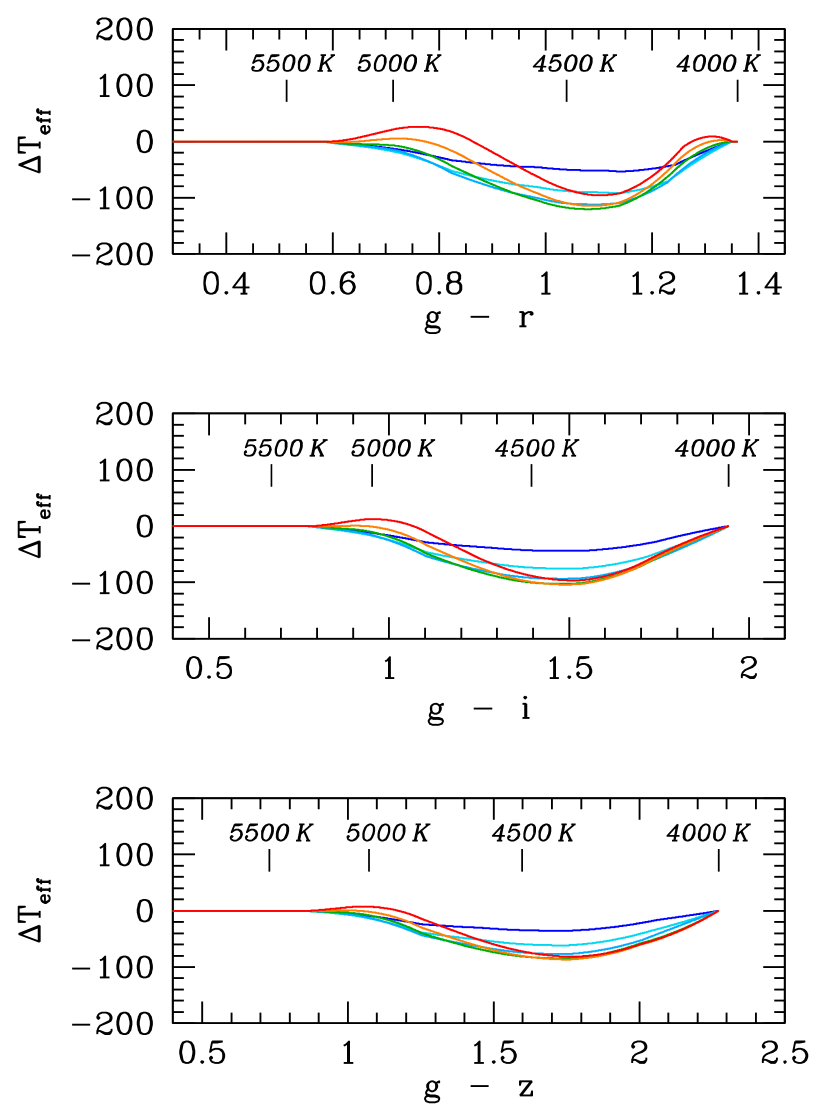
Figure 8.— Theoretical $T_{\rm eff}$ corrections for various $\Delta\log{g}$ values with respect to the fiducial isochrones. Corrections from $\Delta\log{g}=0.5$ (blue) to $\Delta\log{g}=3.0$ (red) with a $0.5$ dex increment are shown. The sense is that giants tend to have lower $T_{\rm eff}$ than dwarfs at fixed colors. A linear ramp was used to define smoothly varying $\Delta T_{\rm eff}$ over $4800$ K $<T_{\rm eff}<5800$ K. In this revision, a simple quadratic relation is used to extend theoretical $T_{\rm eff}$ corrections to the very cool end ($g\,-\,r\gtrsim 1.25$), where correction factors become zero at $T_{\rm eff}\sim 4000$ K. Only a minor fraction of giants in the sample ($\sim 400$ stars) are affected by this change.

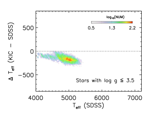
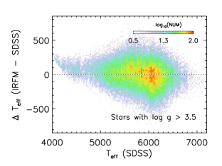
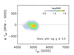
Figure 18.— Comparisons of $T_{\rm eff}$ using the final SDSS $T_{\rm eff}$ estimates. Comparisons are shown for the original KIC $T_{\rm eff}$ for dwarfs (top left) and giants (top right), and for the $(J\,-\,K_{s})$-based IRFM estimates for dwarfs (bottom left) and giants (bottom right). Comparisons for giants shown in the right panels are affected by the sign flip errors in the gravity corrections, but comparisons for dwarfs in the left panels are unaffected.

References

- Aihara et al. (2011) Aihara, H., et al. 2011, ApJS, 193, 29
- An et al. (2007a) An, D., Terndrup, D. M., & Pinsonneault, M. H. 2007a, ApJ, 671, 1640
- An et al. (2007b) An, D., Terndrup, D. M., Pinsonneault, M. H., Paulson, D. B., Hanson, R. B., & Stauffer, J. R. 2007b, ApJ, 655, 233
- An et al. (2008) An, D., et al. 2008, ApJS, 179, 326
- An et al. (2009a) An, D., et al. 2009a, ApJ, 700, 523 (A09)
- An et al. (2009b) An, D., et al. 2009b, ApJ, 707, L64
- Barrado y Navascués et al. (2001) Barrado y Navascués, D., Stauffer, J. R., Bouvier, J., & Martín, E. L. 2001, ApJ, 546, 1006
- Brown et al. (2011) Brown, T. M., Latham, D. W., Everett, M. E., & Esquerdo, G. A. 2011, AJ, 142, 112
- Bruntt et al. (2010) Bruntt, H., Bedding, T. R., Quirion, P.-O., et al. 2010, MNRAS, 405, 1907
- Bruntt et al. (2011) Bruntt, H. et al. 2011, MNRAS, submitted (B11)
- Cardelli et al. (1989) Cardelli, J. A., Clayton, G. C., & Mathis, J. S. 1989, ApJ, 345, 245
- Casagrande et al. (2010) Casagrande, L., Ramírez, I., Meléndez, J., Bessell, M., & Asplund, M. 2010, A&A, 512, A54 (C10)
- Casagrande et al. (2011) Casagrande, L. et al. 2011, A&A, 530, A138
- Castelli & Kurucz (2004) Castelli, F., & Kurucz, R. L. 2004, arXiv:astro-ph/0405087
- Chaplin et al. (2011) Chaplin, W.J. et al. 2011, Science, 332, 213
- Clem et al. (2008) Clem, J. L., Vanden Berg, D. A., & Stetson, P. B. 2008, AJ, 135, 682
- Girardi et al. (2002) Girardi, L., Bertelli, G., Bressan, A., Chiosi, C., Groenewegen, M. A. T., Marigo, P., Salasnich, B., & Weiss, A. 2002, A&A, 391, 195
- Girardi et al. (2004) Girardi, L., Grebel, E. K., Odenkirchen, M., & Chiosi, C. 2004, A&A, 422, 205
- Grevesse & Sauval (1998) Grevesse, N., & Sauval, A. J. 1998, Space Sci. Rev., 85, 161
- Lejeune et al. (1997) Lejeune, Th., Cuisinier, F. & Buser, R. 1997, A&AS, 125, 229
- Lejeune et al. (1998) Lejeune, Th., Cuisinier, F. & Buser, R. 1998, A&AS, 130, 65
- Marigo et al. (2008) Marigo, P., Girardi, L., Bressan, A., et al. 2008, A&A, 482, 883
- Metcalfe et al. (2010) Metcalfe, T. S., Monteiro, M. J. P. F. G., Thompson, M. J., et al. 2010, ApJ, 723, 1583
- Molenda-Żakowicz et al. (2007) Molenda-Żakowicz, J., Frasca, A., Latham, D.W. & Jerzykiewicz, M. 2007, Acta. Astron., 57, 301
- Molenda-Żakowicz et al. (2011) Molenda-Żakowicz, J., Latham, D. W., Catanzaro, G., Frasca, A., & Quinn, S. N. 2011, MNRAS, 412, 1210 (MZ11)
- Montgomery et al. (1993) Montgomery, K. A., Marschall, L. A., & Janes, K. A. 1993, AJ, 106, 181
- Nordstrom et al. (2004) Nordstrom, B., Mayor, M., Anderson, J., Holmberg, J., Pont, F., Jorgensen, B. R., Olsen, E.H., Udry, S. & Mowlavi, N. 2004, A&A, 418, 989
- Oke & Gunn (1983) Oke, J. B., & Gunn, J. E. 1983, ApJ, 266, 713
- Pinsonneault et al. (2003) Pinsonneault, M. H., Terndrup, D. M., Hanson, R. B., & Stauffer, J. R. 2003, ApJ, 598, 588
- Pinsonneault et al. (2004) Pinsonneault, M. H., Terndrup, D. M., Hanson, R. B., & Stauffer, J. R. 2004, ApJ, 600, 946
- Sandquist (2004) Sandquist, E. L. 2004, MNRAS, 347, 101
- Skrutskie et al. (2006) Skrutskie, M. F., et al. 2006, AJ, 131, 1163
- Stauffer et al. (2003) Stauffer, J. R., Jones, B. F., Backman, D., Hartmann, L. W., Barrado y Navascués, D., Pinsonneault, M. H., Terndrup, D. M., & Muench, A. A. 2003, AJ, 126, 833
- Stetson et al. (2003) Stetson, P. B., Bruntt, H., & Grundahl, F. 2003, PASP, 115, 413
- VandenBerg et al. (2010) VandenBerg, D. A., Casagrande, L., & Stetson, P. B. 2010, AJ, 140, 1020