Microlocal Analysis of an Ultrasound Transform with Circular Source and Receiver Trajectories

Abstract.

In this article, we consider a generalized Radon transform that comes up in ultrasound reflection tomography. In our model, the ultrasound emitter and receiver move at a constant distance apart along a circle. We analyze the microlocal properties of the transform $\mathcal{R}$ that arises from this model. As a consequence, we show that for distributions with support sufficiently inside the circle, $\mathcal{R}^{*}\mathcal{R}$ is an elliptic pseudodifferential operator of order $-1$ and hence all the singularities of such distributions can be recovered.

1. Introduction

Ultrasound reflection tomography (URT) is one of the safest and most cost effective modern medical imaging modalities (e.g. see [9, 10, 11, 12] and the references there). During its scanning process, acoustic waves emitted from a source reflect from inhomogeneities inside the body, and their echoes are measured by a receiver. This measured data is then used to recover the unknown ultrasonic reflectivity function, which is used to generate cross-sectional images of the body.

In a typical setup of ultrasound tomography, the emitter and receiver are combined into one device (transducer). The transducer emits a short acoustic pulse into the medium, and then switches to receiving mode, recording echoes as a function of time. Assuming that the medium is weakly reflecting (i.e. neglecting multiple reflections), and that the speed of sound propagation $c$ is constant, the echoes measured at time $t$ uniquely determine the integrals of the reflectivity function over concentric spheres centered at the transducer location and radii $r=ct/2$ (see Fig. 1 (a) below, [12] and the references there). By focusing the transducer one can consider echoes coming only from a certain plane, hence measuring the integrals of the reflectivity function in that plane along circles centered at the transducer location [11]. Moving the transducer along a curve on the edge of the body, and repeating the measurements one obtains a two-dimensional family of integrals of the unknown function along circles. Hence the problem of image reconstruction in URT can be mathematically reduced to the problem of inverting a circular Radon transform, which integrates an unknown function of two variables along a two-dimensional family of circles.

In the case when the emitter and receiver are separated, the echoes recorded by a transducer correspond to the integrals of the reflectivity function along confocal ellipses with foci corresponding to the locations of the emitter and receiver (see Fig. 1 (b)). While this more general setup has been gaining popularity in recent years (e.g. see [9, 10]), the mathematical theory related to elliptical Radon transforms is relatively undeveloped. In this paper we study the microlocal properties of this transform which integrates an unknown function along a family of ellipses.

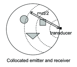
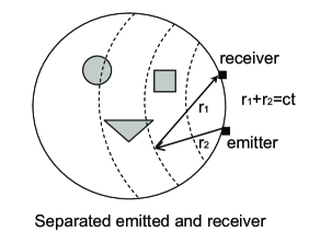
Figure 1. A sketch of integrating curves in URT

2. Definitions and Preliminaries

We will first define the elliptical Radon transform we consider, provide the general framework for the microlocal analysis of this transform, and show that our transform fits within this framework.

2.1. The Elliptical Transform

In URT the locations of the emitter and receiver are limited to a curve surrounding the support of the function to be recovered and the data taken can be modeled as integrals of the reflectivity function of the object over ellipses with foci being the transmitter and the receiver. In this paper we consider this curve to be a circle, which is both the simplest case mathematically and the one most often used in practice. By using a dilation, we can assume the circle has radius $r=1$. We also make the restriction that the source and detector rotate around the circle a fixed distance apart. We denote the fixed difference between the polar angles of emitter and receiver by $2\alpha$, where $\alpha\in(0,\pi/2)$ (see Fig. 2) and define

$$a=\sin\alpha,\qquad b=\cos\alpha.$$ (2.1)

As we will see later our main result relies on the assumption that the support of the function is small enough. More precisely, we will assume our function is supported in the ball

$$\mathrm{D}_{b}=\{x\in{\mathbb{R}}^{2}\hskip 0.85358pt\big{|}\hskip 0.85358pt|x|<b\}.$$

We parameterize the trajectories of the emitter and receiver, respectively, as

$$\gamma_{T}(s) =(\cos(s-\alpha),\sin(s-\alpha))$$

$$\gamma_{R}(s) =(\cos(s+\alpha),\sin(s+\alpha))\quad\text{for $s\in[0,2\pi].$}$$

Thus, the emitter and receiver rotate around the unit circle and are always $2a$ units apart. For $s\in[0,2\pi]$ and $L>2a$, let

$$E(s,L)=\{x\in{\mathbb{R}}^{2}\hskip 0.85358pt\big{|}\hskip 0.85358pt|x-\gamma_{T}(s)|+|x-\gamma_{R}(s)|=L\}.$$

Note that the center of the ellipse $E(s,L)$ is $(b\cos s,b\sin s)$ and $L$ is the diameter of the major axis of $E(s,L)$, the so called major diameter. This is why we require $L$ to be greater than the distance between the foci, $2a$. Note that $E(0,L)=E(2\pi,L)$ and so $[0,2\pi]$ can be viewed as the unit circle.

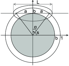
Figure 2. A sketch of the domain and the notations

Let

$$Y=\{(s,L)\hskip 0.85358pt\big{|}\hskip 0.85358pts\in[0,2\pi],\ L>2a\},$$

then $Y$ is the set of parameters for the ellipses.

Definition 2.1.

Let $(s,L)\in Y$. The elliptical Radon transform of a locally integrable function $f:{\mathbb{R}}^{2}\to\mathbb{R}$ is defined as

$$\mathcal{R}f(s,L)=\int\limits_{x\in E(s,L)}f(x)\mathrm{d}l(x)$$

where $\mathrm{d}l$ is the arc length measure on the ellipse $E(s,L)$.

The backprojection transform is defined for $g\in C_{c}(Y)$ as

$$\mathcal{R}^{*}g(x)=\int_{s\in[0,2\pi]}g(s,|x-\gamma_{R}(s)|+|x-\gamma_{T}(s)|)\mathrm{d}s$$

where the positive smooth measure $\mathrm{d}s$ is chosen so that $\mathcal{R}^{*}$ is the $L^{2}$ adjoint of $\mathcal{R}$. Note that $\mathcal{R}^{*}$ integrates over a compact set, $[0,2\pi]$ (or the circle), and so $\mathcal{R}^{*}$ can be composed with $\mathcal{R}$. Using the parametrization of ellipses $(s,L)$ one sees that $\mathcal{R}^{*}g(x)$ integrates (with a smooth measure) over the set of all ellipses passing through $x$.

We now briefly discuss the general framework of Guillemin and Sternberg into which our elliptical Radon transform falls. We use this to understand the microlocal analysis of $\mathcal{R}$. We begin with some general notation we will use when we discuss microlocal analysis.

2.2. Microlocal Definitions

Let $X$ and $Y$ be smooth manifolds and let

$${\mathcal{C}}\subset T^{*}(Y)\times T^{*}(X),$$

then we let

$${\mathcal{C}}^{\prime}=\{(y,\eta,x,\xi)\hskip 0.85358pt\big{|}\hskip 0.85358pt(y,\eta,x,-\xi)\in{\mathcal{C}}\}.$$

The transpose relation is ${\mathcal{C}}^{t}\subset T^{*}(X)\times T^{*}(Y)$:

$${\mathcal{C}}^{t}=\{(x,\xi,y,\eta)\hskip 0.85358pt\big{|}\hskip 0.85358pt(y,\eta,x,\xi)\in{\mathcal{C}}\}$$

If ${\mathcal{D}}\subset T^{*}(X)\times T^{*}(Y)$, then the composition ${\mathcal{D}}\circ{\mathcal{C}}$ is defined

$${\mathcal{D}}\circ{\mathcal{C}} =\{(x^{\prime},\xi^{\prime},x,\xi)\hskip 0.85358pt\big{|}\hskip 0.85358pt\exists(y,\eta)\in T^{*}(Y)$$

$$\qquad\text{with }(x^{\prime},\xi^{\prime},y,\eta)\in{\mathcal{D}},\ (y,\eta,x,\xi)\in{\mathcal{C}}\}.$$

2.3. The Radon Transform and Double Fibrations

Guillemin first put the Radon transform into a microlocal framework, and we will use this approach to prove Theorem 3.1. These results were first given in the technical report [4] (some of which appeared in [5]), then outlined in [6, pp. 336-337, 364-365]. The dependence on the measures and details of the proofs for the case of equal dimensions were given in [13]. Guillemin used the ideas of push-forwards and pullbacks to define Radon transforms in [4] and he used these ideas to define Fourier integral operators (FIOs) [4, 6]. Finally Guillemin summarized this material in [5].

Given smooth connected manifolds $X$ and $Y$ of the same dimension, let $Z\subset Y\times X$ be a smooth connected submanifold of codimension $k<\dim(X)$. We assume that the natural projections

$${\begin{matrix}&Z&\\ &{\hbox to0.0pt{\hss$\raisebox{6.0pt}{\hbox{\hbox{$\scriptstyle{\pi_{L}}$}}}$}{\swarrow}\ \qquad{\mathbf{\searrow}}\hbox to0.0pt{$\raisebox{6.0pt}{\hbox{\hbox{$\scriptstyle{\pi_{R}}$}}}$\hss}}&\\ {Y}&&{X}&\end{matrix}}$$ (2.2)

are both fiber maps. In this case, we call (2.2) a double fibration.

Following Guillemin and Sternberg, we assume that $\pi_{R}$ is a proper map; that is, the fibers of $\pi_{R}:Z\to X$ are compact. The double fibration allows us to define a Radon transform as follows. For each $y\in Y$ let

$$E(y)=\pi_{R}\left(\pi_{L}^{-1}(\{y\})\right),$$

then the sets $E(y)$ are all diffeomorphic to the fiber of the fibration $\pi_{L}:Z\to Y$. For each $x\in X$ let

$$F(x)=\pi_{L}\left(\pi_{R}^{-1}(\{x\})\right),$$

and the sets $F(x)$ are all diffeomorphic to the fiber of $\pi_{R}:Z\to X$. Since $\pi_{R}$ is proper, the sets $F(x)$ are compact. By choosing smooth nowhere zero measures on $Z$, $X$, and on $Y$, one can then define a smooth nowhere zero measure $\mu_{y}$ on $E(y)$ and $\mu_{x}$ on $F(x)$ and a Radon transform

$$Rf(y)=\int_{x\in E(y)}f(x)\mathrm{d}\mu_{y}(x)$$

and the dual transform is

$$R^{*}g(x)=\int_{y\in F(x)}g(y)\mathrm{d}\mu_{x}(y)$$

[6] (see also [13, p. 333]). Since the sets $F(x)$ are compact, one can compose $R^{*}$ and $R$ for $f\in C_{c}(X)$. If $\pi_{R}$ is not a proper map, then one needs cutoff functions to compose $R^{*}$ with $R$. We assume $E(y_{1})=E(y_{2})$ if and only if $y_{1}=y_{2}$ and similarly for $F$.

Guillemin showed ([4, 5] and with Sternberg [6]) that $R$ is a Fourier integral distribution associated with integration over $Z$ and canonical relation ${\mathcal{C}}=(N^{*}(Z){\setminus\{\boldsymbol{0}}\})^{\prime}$. To understand the properties of $R^{*}R$, one must investigate the mapping properties of ${\mathcal{C}}$. Let $\Pi_{L}:{\mathcal{C}}\to T^{*}(Y)$ and $\Pi_{R}:{\mathcal{C}}\to T^{*}(X)$ be the natural projections. Then we have the following diagram:

$${\begin{matrix}&{\mathcal{C}}&\\ &{\hbox to0.0pt{\hss$\raisebox{6.0pt}{\hbox{\hbox{$\scriptstyle{\Pi_{L}}$}}}$}{\swarrow}\ \qquad{\mathbf{\searrow}}\hbox to0.0pt{$\raisebox{6.0pt}{\hbox{\hbox{$\scriptstyle{\Pi_{R}}$}}}$\hss}}&\\ {T^{*}(Y)}&&{T^{*}(X)}&\end{matrix}}$$ (2.3)

This diagram is the microlocal version of (2.2).

Definition 2.2 ([4, 5]).

Let $X$ and $Y$ be manifolds with $\dim(Y)=\dim(X)$ and let ${\mathcal{C}}\subset(T^{*}(Y)\times T^{*}(X)){\setminus\{\boldsymbol{0}}\}$ be a canonical relation. Then, ${\mathcal{C}}$ satisfies the Bolker Assumption if

$$\Pi_{Y}:{\mathcal{C}}\to T^{*}(Y)$$

is an injective immersion.

This definition was originally proposed by Guillemin [4],[5, p. 152], [6, p. 364-365] because a similar assumption for the Radon transform on finite sets implies $R^{*}R$ is injective in this case. Guillemin proved that if the measures that define the Radon transform are smooth and nowhere zero, and if the Bolker Assumption holds (and $R$ is defined by a double fibration for which $\pi_{R}$ is proper), then $R^{*}R$ is an elliptic pseudodifferential operator.

In the definition in [4, 13], the dimensions of $X$ and $Y$ are equal, but in [5], $\dim(Y)\geq\dim(X)$. We use the former definition since, in our case, $\dim(Y)=\dim(X)$. Since we assume $\dim(Y)=\dim(X)$, if $\Pi_{Y}:{\mathcal{C}}\to T^{*}(Y)$ is an injective immersion, then $\Pi_{Y}$ maps to $T^{*}(Y){\setminus\{\boldsymbol{0}}\}$ and $\Pi_{X}$ is also an immersion [7]. Therefore, $\Pi_{X}$ maps to $T^{*}(X){\setminus\{\boldsymbol{0}}\}$. So, under the Bolker Assumption, ${\mathcal{C}}\subset(T^{*}(Y){\setminus\{\boldsymbol{0}}\})\times(T^{*}(X){\setminus\{\boldsymbol{0}}\})$ and so $R$ is a Fourier integral operator according to the definition in [14].

For our transform $\mathcal{R}$, the incidence relation is

$$Z=\{(s,L,x)\subset Y\times\mathrm{D}_{b}\hskip 0.85358pt\big{|}\hskip 0.85358ptx\in E(s,L)\}.$$ (2.4)

The double fibration is

$${\begin{matrix}&Z&\\ &{\hbox to0.0pt{\hss$\raisebox{6.0pt}{\hbox{\hbox{$\scriptstyle{\pi_{L}}$}}}$}{\swarrow}\ \qquad{\mathbf{\searrow}}\hbox to0.0pt{$\raisebox{6.0pt}{\hbox{\hbox{$\scriptstyle{\pi_{R}}$}}}$\hss}}&\\ {Y}&&{\mathrm{D}_{b}}&\end{matrix}}$$ (2.5)

and both projections are fiber maps. Note that the fibers of $\pi_{L}$ are ellipses, $E(s,L)=\pi_{R}(\pi_{L}^{-1}(\{(s,L)\})$. Furthermore, the fibers of $\pi_{R}$ are diffeomorphic to $[0,2\pi]$ or the circle, so $\pi_{R}$ is proper. Therefore $\mathcal{R}$ and $\mathcal{R}^{*}$ satisfy the conditions outlined above so that Guillemin and Sternberg’s framework can be applied.

3. The Main Result

We now state the main result of this article.

Theorem 3.1.

Let $\alpha>0$ be a constant and let $\gamma_{T}(s)=(\cos(s-\alpha),\sin(s-\alpha))$ and $\gamma_{R}(s)=(\cos(s+\alpha),\sin(s+\alpha))$ for $s\in[0,2\pi]$ be the trajectories of the emitter and receiver respectively. Denote by $\mathcal{E}^{\prime}(\mathrm{D}_{b})$ the space of compactly supported distributions supported in the disc, $\mathrm{D}_{b}$, of radius $b$ centered at $0$, where $b=\cos\alpha$. The elliptical Radon transform $\mathcal{R}$ when restricted to the domain $\mathcal{E}^{\prime}(\mathrm{D}_{b})$ satisfies the microlocal conditions in Section 2.3, and $\mathcal{R}$ is an elliptic Fourier integral operator (FIO) of order $-1/2$. Let ${\mathcal{C}}\subset T^{*}(Y)\times T^{*}(\mathrm{D}_{b})$ be the canonical relation associated to $\mathcal{R}$. Then, ${\mathcal{C}}$ satisfies the Bolker Assumption (Definition 2.2).

As a consequence of this result, we have the following corollary.

Corollary 3.1.

The composition of $\mathcal{R}$ with its $L^{2}$ adjoint $\mathcal{R}^{*}$ when restricted as a transformation from ${\mathcal{E}}^{\prime}(\mathrm{D}_{b})$ to ${\mathcal{D}}^{\prime}(\mathrm{D}_{b})$ is an elliptic pseudo-differential operator of order $-1$.

Remark 3.2.

This corollary shows that, for $\operatorname{supp}f\subset\mathrm{D}_{b}$, the singularities of $\mathcal{R}^{*}\mathcal{R}f$ are at the same locations and co-directions as the singularities of $f$, that is, the wavefront sets are the same. In other words, $\mathcal{R}^{*}\mathcal{R}$ reconstructs all the singularities of $f$. If $D$ is an elliptic differential operator on $Y$, then one can create an elliptic local reconstruction operator $\mathcal{R}^{*}D\mathcal{R}$ that will emphasize singularities. REU research student Howard Levinson [8] refined and implemented an algorithm of Prof. Quinto’s of this form and the algorithm does show all the singularities of $f$. Because of the derivative, the algorithm highlights boundaries, and this type of algorithm generalizes Lambda Tomography [3, 2].

4. Proofs of Theorem 3.1 and Corollary 3.1

Proof of Theorem 3.1.

First, we will calculate ${\mathcal{C}}=(N^{*}(Z){\setminus\{\boldsymbol{0}}\})^{\prime}$ where $Z$ is given by (2.4). Then most of the proof is devoted to showing that ${\mathcal{C}}$ satisfies the Bolker Assumption.

Since $Z$ is defined by the equation

$$L-|x-\gamma_{R}(s)|-|x-\gamma_{T}(s)|=0,$$

the differential of the function is a basis for $N^{*}(Z)$. That differential is

$$=-\left(\frac{x\cdot\gamma_{R}^{\prime}(s)}{|x-\gamma_{R}(s)|}+\frac{x\cdot\gamma_{T}^{\prime}(s)}{|x-\gamma_{T}(s)|}\right)\mathrm{d}s+\mathrm{d}L$$

$$\qquad-\left(\frac{x-\gamma_{R}(s)}{|x-\gamma_{R}(s)|}+\frac{x-\gamma_{T}(s)}{|x-\gamma_{T}(s)|}\right)\mathrm{d}x.$$

Note that we are using the fact that $\gamma_{R}(s)$ and $\gamma_{R}^{\prime}(s)$ are orthogonal (as are $\gamma_{T}(s)$ and $\gamma_{T}^{\prime}(s)$). Therefore, ${\mathcal{C}}=\left(N^{*}(Z){\setminus\{\boldsymbol{0}}\}\right)^{\prime}$ is

$${\mathcal{C}}=\Bigg{\{}\Bigg{(}s,L,\omega\left(-\left(\frac{x\cdot\gamma_{R}^{\prime}(s)}{|x-\gamma_{R}(s)|}+\frac{x\cdot\gamma_{T}^{\prime}(s)}{|x-\gamma_{T}(s)|}\right)\mathrm{d}s+\mathrm{d}L\right),$$ (4.1)

$$\qquad\qquad x,\omega\left(\frac{x-\gamma_{R}(s)}{|x-\gamma_{R}(s)|}+\frac{x-\gamma_{T}(s)}{|x-\gamma_{T}(s)|}\right)\mathrm{d}x\Bigg{)}$$

$$\qquad\qquad\qquad\qquad\hskip 0.85358pt\big{|}\hskip 0.85358pt(s,L,x)\in Z,\ \omega\in\mathbb{R}\setminus\{0\}\Bigg{\}}.$$

The Schwartz kernel of $\mathcal{R}$ is integration on $Z$ (e.g., [13, Proposition 1.1]) and so is a Fourier integral distribution associated to ${\mathcal{C}}$ [5].

Now we show that the projection $\Pi_{L}$ satisfies the Bolker Assumption. If $\lambda\in{\mathcal{C}}$ the projection is given by (4.1)

$$\Pi_{L}(\lambda)=\left(s,L,\omega\left(-\left(\frac{x\cdot\gamma_{R}^{\prime}(s)}{|x-\gamma_{R}(s)|}+\frac{x\cdot\gamma_{T}^{\prime}(s)}{|x-\gamma_{T}(s)|}\right)\mathrm{d}s+\mathrm{d}L\right)\right).$$

From this, we have determined, $s$, $L$, and $\omega$ and we need to find $x$ knowing that $x\in E(s,L)$.

The easiest way to do this is to develop coordinates, first on the ellipses, then on $Z$, and finally on ${\mathcal{C}}$.

We will reduce to the case $s=\pi/2$, so first we give coordinates on the ellipse $E(\pi/2,L)$ (see Figure 3), which has foci $(\pm a,b)$: for $\phi\in[0,2\pi]$ and $L>2a$ we define

$$\begin{gathered}x^{\prime}=x^{\prime}(L,\phi)=(a\cosh\rho\cos\phi,b+a\sinh\rho\sin\phi)\\ \text{where}\ \ \rho=\arccos(2L/a).\end{gathered}$$ (4.2)

Figure 3. Elliptic Coordinate System. The radius of the circle in the figure is $b$.

Note that the ellipse $E(s,L)$ meets the ball $\mathrm{D}_{b}$ if and only if $L\in(2a,2\sqrt{a^{2}+4b^{2}})$, and for each $L\in(2a,2\sqrt{a^{2}+4b^{2}})$, there is an interval $(\phi_{\min}(L),\phi_{\max}(L))$ with $\pi<\phi_{\min}(L)<\phi_{\max}(L)<2\pi$ such that $x^{\prime}(L,\phi)\in\mathrm{D}_{b}$ if and only if $\phi\in(\phi_{\min}(L),\phi_{\max}(L))$.

Next we let $T_{\theta}$ be the counterclockwise rotation about the origin through $\theta$ radians. For $(s,L)\in Y$, this gives coordinates on the ellipse $E(s,L)$

$$x(s,L,\phi)=T_{s-\pi/2}\left(x^{\prime}(L,\phi)\right)$$

since $T_{s-\pi/2}$ rotates $\gamma_{R}(\pi/2)$ to $\gamma_{R}(s)$ and rotates $\gamma_{T}(\pi/2)$ to $\gamma_{T}(s)$. This rotation preserves distances and so it does not change the major diameter of the ellipse, $L$. Furthermore, for $\phi\in(\phi_{\min}(L),\phi_{\max}(L))$, $x(s,L,\phi)\in\mathrm{D}_{b}$.

We get coordinates on $Z$ as follows. Let

$$\tilde{Z}=\{(s,L,\phi)\hskip 0.85358pt\big{|}\hskip 0.85358pts\in[0,2\pi],\ L\in(2a,2\sqrt{a^{2}+4b^{2}}),$$

$$\phi\in(\phi_{\min}(L),\phi_{\max}(L))\}.$$

This provides local coordinates above $\mathrm{D}_{b}$ on $Z$:

$$\tilde{Z}\ni(s,L,\phi)\mapsto z(s,L,\phi)=\left(s,L,x(s,L,\phi)\right).$$

Finally, this gives coordinates on ${\mathcal{C}}$:

$$\lambda(s,L,\phi,\omega) =(s,L,\omega\left(-\left(\frac{x\cdot\gamma_{R}^{\prime}(s)}{|x-\gamma_{R}(s)|}+\frac{x\cdot\gamma_{T}^{\prime}(s)}{|x-\gamma_{T}(s)|}\right)\mathrm{d}s+\mathrm{d}L\right),$$

$$\qquad\qquad x,\omega\left(\frac{x-\gamma_{R}(s)}{|x-\gamma_{R}(s)|}+\frac{x-\gamma_{T}(s)}{|x-\gamma_{T}(s)|}\right)\mathrm{d}x\big{)}$$

$$\text{where}\ \ (s,L,\phi,\omega)\in\tilde{Z}\times(\mathbb{R}\setminus\{0\}),$$

$$\text{and}\ x=x(s,L,\phi)$$

and this gives $\Pi_{L}$ in coordinates as

$$\Pi_{L}(\lambda(s,L,\phi,\omega)) =\Big{(}s,L,-\omega\left(\frac{x\cdot\gamma_{R}^{\prime}(s)}{|x-\gamma_{R}(s)|}+\frac{x\cdot\gamma_{T}^{\prime}(s)}{|x-\gamma_{T}(s)|}\right)\mathrm{d}s$$

$$\qquad+\omega\mathrm{d}L\Big{)}.$$

Using a series of estimates, we will show the following claim.

Claim 4.1.

For $(s,L,\phi)\in\tilde{Z}$, the derivative of

$$\frac{x(s,L,\phi)\cdot\gamma_{R}^{\prime}(s)}{|x(s,L,\phi)-\gamma_{R}(s)|}+\frac{x(s,L,\phi)\cdot\gamma_{T}^{\prime}(s)}{|x(s,L,\phi)-\gamma_{T}(s)|}$$ (4.3)

with respect to $\phi$ is never zero.

This claim shows that $\Pi_{L}$ is injective for the following reasons. Since $s,L$ and $\omega\neq 0$ are given from the projection $\Pi_{L}$, to show $\Pi_{L}$ is injective, all we need to show is that for fixed $(s,L)$ with $s\in[0,2\pi]$ and $L\in(2a,2\sqrt{a^{2}+4b^{2}}),$ (4.3) determines $\phi\in{(\phi_{\min}(L),\phi_{\max}(L))}$ uniquely. However, Claim 4.1 shows for fixed $(s,L)$ and $\phi$ in the interval ${(\phi_{\min}(L),\phi_{\max}(L))}$ that (4.3) is either strictly increasing or strictly decreasing. Since ${(\phi_{\min}(L),\phi_{\max}(L))}$ is an interval, this will show that (4.3) is an injective function of $\phi$ and therefore $\Pi_{L}$ is injective.

Next, we will use Claim 4.1 to argue that $\Pi_{L}$ is an immersion. Since $s,L$ and $\omega\neq 0$ are given directly from the projection $\Pi_{L}$, writing out the derivative matrix of $\Pi_{L}$ shows that one only needs to prove for $(s,L,\phi)\in\tilde{Z}$ and $\omega\neq 0$ that the derivative of (4.3) with respect to $\phi$ is nowhere zero. This again follows from the claim.

Proof of Claim 4.1.

We prove this by making a reduction to $s=\pi/2$ and then by a series of estimates.

Using rotation invariance: we apply $T_{\pi/2-s}$ on ${\mathbb{R}}^{2}$, and use the facts that distances and dot products are preserved (so e.g., $x\cdot\gamma_{R}^{\prime}(s)=x^{\prime}\cdot\gamma_{R}^{\prime}(\pi/2)$ and $|x-\gamma_{R}(s)|=|x^{\prime}-\gamma_{R}(\pi/2)|$) where

$$\begin{gathered}T_{\pi/2-s}(x(s,L,\phi))=x^{\prime}(L,\phi),\\ T_{\pi/2-s}(\gamma_{R}(s))=\gamma_{R}(\pi/2)=(-a,b),\\ T_{\pi/2-s}(\gamma_{R}^{\prime}(s))=\gamma_{R}^{\prime}(\pi/2)=(-b,-a))\\ T_{\pi/2-s}(\gamma_{T}(s))=\gamma_{T}(\pi/2)=(a,b),\\ T_{\pi/2-s}(\gamma_{T}^{\prime}(s))=\gamma_{T}^{\prime}(\pi/2)=(-b,a)\end{gathered}$$

This gives the simplified expression that is equal to (4.3):

$$S(L,\phi)=\left(\frac{x^{\prime}(L,\phi)\cdot(-b,-a)}{|x^{\prime}(L,\phi)-(-a,b)|}+\frac{x^{\prime}(L,\phi)\cdot(-b,a)}{|x^{\prime}(L,\phi)-(a,b)|}\right).$$

We have reduced showing $\Pi_{L}$ is an injective immersion to showing

$$\begin{gathered}\frac{\partial}{\partial\phi}S(L,\phi)\neq 0\\ \text{ for }L\in(2a,2\sqrt{a^{2}+4b^{2}}),\ \phi\in{(\phi_{\min}(L),\phi_{\max}(L))}.\end{gathered}$$

Using (4.2) we obtain

$$\begin{gathered}|x^{\prime}(L,\phi)-(-a,b)|=\sqrt{a^{2}(\cosh\rho\cos\phi+1)^{2}+a^{2}\sinh^{2}\rho\sin^{2}\phi}\\ =a(\cosh\rho+\cos\phi),\end{gathered}$$

$$\begin{gathered}|x^{\prime}(L,\phi)-(a,b)|=\sqrt{a^{2}(\cosh\rho\cos\phi-1)^{2}+a^{2}\sinh^{2}\rho\sin^{2}\phi}\\ =a(\cosh\rho-\cos\phi)\end{gathered}$$

and

$$S(L,\phi) =\frac{-b\cosh\rho\cos\phi-b-a\sinh\rho\sin\phi}{\cosh\rho+\cos\phi}$$

$$+\frac{-b\cosh\rho\cos\phi+b+a\sinh\rho\sin\phi}{\cosh\rho-\cos\phi}.$$

Adding these two fractions, and simplifying the expression yields the following:

$$S(L,\phi)=H(\rho,\phi)=\displaystyle{\frac{2\sinh\rho\,\cos\phi\;(a\sin\phi-b\sinh\rho)}{(\cosh\rho+\cos\phi)(\cosh\rho-\cos\phi)}}$$

Our problem therefore is reduced to showing that $\frac{\partial}{\partial\phi}H(\rho,\phi)\neq 0$.

Denote $t=\cos\phi$, then $\sin\phi=-\sqrt{1-t^{2}}$, since $\phi\in[\pi,2\pi]$.

Consider a new function $\tilde{H}(t)$ defined as follows (the term $-2\sinh\rho$ does not matter):

$$\tilde{H}(t)=\displaystyle{\frac{b\,\sinh\rho t+at\sqrt{1-t^{2}}}{\cosh^{2}\rho-t^{2}}}.$$

$$\tilde{H}^{\prime}(t) =\frac{1}{\left(\cosh^{2}\rho-t^{2}\right)^{2}}\Big{[}2t\left(bt\sinh\rho+at\sqrt{1-t^{2}}\right)$$

$$\quad+\left(b\,\sinh\rho+a\sqrt{1-t^{2}}-\displaystyle\frac{at^{2}}{\sqrt{1-t^{2}}}\right)\left(\cosh^{2}\rho-t^{2}\right)\Big{]}.$$

Denoting the numerator of the above expression by $N$, and distributing the product we get

$$N =\cosh^{2}\rho\left(b\,\sinh\rho+a\sqrt{1-t^{2}}-\frac{at^{2}}{\sqrt{1-t^{2}}}\right)$$ (4.4)

$$\qquad+t^{2}\left(b\sinh\rho+a\sqrt{1-t^{2}}+\frac{at^{2}}{\sqrt{1-t^{2}}}\right)$$

$$=\left(\cosh^{2}\rho+t^{2}\right)\left(b\sinh\rho+a\sqrt{1-t^{2}}\right)-\left(\cosh^{2}\rho-t^{2}\right)\frac{at^{2}}{\sqrt{1-t^{2}}}.$$

Denoting

$$k=\sinh\rho,\ \ \text{we have}\ \ \cosh^{2}\rho=1+k^{2},$$

and

$$N =\sqrt{1-a^{2}}\,k\,(1+k^{2})+a(1+k^{2})\sqrt{1-t^{2}}+\sqrt{1-a^{2}}\;k\,t^{2}$$

$$\qquad+at^{2}\sqrt{1-t^{2}}+\frac{at^{4}}{\sqrt{1-t^{2}}}-\frac{a(1+k^{2})t^{2}}{\sqrt{1-t^{2}}}$$

Notice that all terms in the above expression are non-negative except the last one. Hence, in order to show that $N>0$ it is enough to show that $N_{1}>0$, where

$$N_{1}=a(1+k^{2})\sqrt{1-t^{2}}+at^{2}\sqrt{1-t^{2}}+\displaystyle\frac{at^{4}}{\sqrt{1-t^{2}}}-\displaystyle\frac{a(1+k^{2})t^{2}}{\sqrt{1-t^{2}}}.$$

Since multiplication by $\sqrt{1-t^{2}}$ does not change the algebraic sign, $N>0$ if and only if $\sqrt{1-t^{2}}\;N_{1}>0$, which is equivalent to

$$t^{2}\leq\displaystyle\frac{1+k^{2}}{1+2k^{2}}.$$ (4.5)

Definition 4.1.

We will call the pair $(\rho,\phi)$ admissible if the point defined by elliptic coordinates $(\rho,\phi)$ is located inside $D(0,b)$, the disc of radius $b$ centered at the origin.

We need to show that $N>0$ for all admissible pairs $(\rho,\phi)$.

Lemma 4.2.

If $|\cos\phi|>b$ then $(\rho,\phi)$ is not admissible for any $\rho>0$.

Proof.

Recall the coordinate system $(\rho,\phi)$ (see Fig. 3) for $x=(x_{1},x_{2})$ defined by

$$\left\{\begin{array}[]{l}x_{1}=a\cosh\rho\cos\phi\\ x_{2}=b+a\sinh\rho\sin\phi\end{array}\right.$$ (4.6)

where $a>0$ is fixed, $\rho>0$, and $\phi\in[0,2\pi]$. It is easy to notice that the coordinate curves (hyperbolas) corresponding to fixed values of $\phi$ intersect the disc $D(0,b)$ only for limited values of $\phi$. To find the range of these values consider the following system of equations:

$$\left\{\begin{array}[]{rcl}\left(\displaystyle\frac{x_{1}}{a\cos\phi}\right)^{2}-\left(\displaystyle\frac{x_{2}-b}{a\sin\phi}\right)^{2}&=&1,\;\;\phi\neq\displaystyle\frac{k\pi}{2},\;\;k=0,\ldots,4\\ \\ x_{1}^{2}+x_{2}^{2}&=&b^{2}.\end{array}\right.$$

Simplifying the system one gets a quadratic equation with respect to $(x_{2}-b)$

$$(x_{2}-b)^{2}+2b\sin^{2}\phi(x_{2}-b)+a^{2}\,\sin^{2}\phi\;\cos^{2}\phi=0,$$

which does not have any real roots if $|\tan\phi|<\displaystyle\frac{a}{b}$. Recalling that $b=\sqrt{1-a^{2}}$ we conclude that the hyperbolas corresponding to coordinate curves with constant $\phi$ intersect the domain of the function support $D(0,b)$ only when $|t|\leq b=\sqrt{1-a^{2}}$. ∎

Lemma 4.3.

If $\cosh^{2}\rho>\displaystyle\frac{4-3a^{2}}{a^{2}}$ then $(\rho,\phi)$ is not admissible for any $\phi$.

Proof.

From equations (4.6) it is easy to notice that the coordinate curves (ellipses) corresponding to fixed values of $\rho$ do not intersect the disc $D(0,-b,b)$ if $\rho$ is large. Namely, the largest value of $\rho$ for which the corresponding ellipse intersects the disc satisfies the equation $2b=a\sinh\rho$. Since $\cosh^{2}\rho=1+\sinh^{2}\rho$, and $b^{2}=1-a^{2}$ we get that

$$\cosh^{2}\rho\leq\displaystyle\frac{4-3a^{2}}{a^{2}}$$

for each coordinate ellipse that intersects the disc. ∎

Proposition 4.1.

If $\alpha>0.8$, then for all admissible pairs $(\rho,\phi)$ we have $N>0$.

Proof.

Recall from Lemma 4.3 that for admissible pairs $k^{2}+1\leq\displaystyle\frac{4-3a^{2}}{a^{2}}$, hence $0<k\leq\displaystyle\frac{2\sqrt{1-a^{2}}}{a}$. Consider the right hand side of equation (4.5)

$$f(k)=\frac{1+k^{2}}{1+2k^{2}}.$$

The function $f(k)$ is monotonically decreasing and for admissible pairs reaches its minimum

$$f(k_{\mathrm{min}})=\displaystyle\frac{4-3a^{2}}{8-7a^{2}},\;\;k_{\mathrm{min}}=\displaystyle\frac{2\sqrt{1-a^{2}}}{a}.$$

Hence, if we show that under the conditions of the theorem

$$t^{2}<\displaystyle\frac{4-3a^{2}}{8-7a^{2}}$$ (4.7)

then by equation (4.5) and the preceding argument $N>0$. At the same time by Lemma 4.2 we know that $t^{2}<1-a^{2}$. So if $a>0$ satisfies

$$1-a^{2}<\displaystyle\frac{4-3a^{2}}{8-7a^{2}},$$ (4.8)

then (4.7) is satisfied. To finish the proof, notice that the hypothesis of the proposition $\alpha>0.8$ implies (4.8). ∎

Proposition 4.2.

If $\alpha<1.2$, then for all admissible pairs $(\rho,\phi)$ we have $N>0$.

Proof.

From Lemma 4.2, we need to consider only those pairs $(\rho,\phi)$ for which $|t|\leq b$, where $t=\cos\phi$. We will show that $N$ is positive for this range of $t$.

The term $N$ in (4.4) can be rewritten as

$$N(t)=b\sqrt{1-t^{2}}\sinh\rho(\cosh^{2}\rho+t^{2})+a(\cosh^{2}\rho-t^{2}(\cosh^{2}\rho+\sinh^{2}\rho))$$ (4.9)

Using the fact that $b\geq\lvert t\rvert$, we have $\sqrt{1-t^{2}}\geq\sqrt{1-b^{2}}=a$ and we substitute this into (4.9) and use the fact that $b=\sqrt{1-a^{2}}$ to get

$$N(t)\geq ba\sinh\rho(\cosh^{2}\rho+t^{2})+a(\cosh^{2}\rho-t^{2}(\cosh^{2}\rho+\sinh^{2}\rho).$$

Factoring $a$, we are left with wanting to show that

$$b\sinh\rho(\cosh^{2}\rho+t^{2})+\cosh^{2}\rho-t^{2}(\cosh^{2}\rho+\sinh^{2}\rho)\geq 0.$$

Isolating $t^{2}$, we need to show that

$$\frac{(b\sinh\rho+1)\cosh^{2}\rho}{\cosh^{2}\rho+\sinh^{2}\rho-b\sinh\rho}\geq t^{2}.$$ (4.10)

(Note that the term $\cosh^{2}\rho+\sinh^{2}\rho-b\sinh\rho$ is always positive.) We show that for $b\geq\frac{1}{2\sqrt{2}}$, the left hand side of (4.10) is greater than $1$. Solving the inequality by let $x=\sinh\rho$ we get the quadratic inequality

$$bx^{2}-x+2b\geq 0\qquad\text{ with roots }\ x=\frac{1\pm\sqrt{1-8b^{2}}}{2b}.$$

There are no roots if $1<8b^{2}$ or $1/(2\sqrt{2})<b$. Since $b=\cos\alpha$, this corresponds to $\alpha<1.21$ radians. ∎

We have now proved Claim 4.1, and from the discussion following this claim, we have that $\Pi_{L}$ is an injective immersion: the Bolker Assumption holds.∎

Now that we know the Bolker Assumption holds, as mentioned after Definition 2.2, the projections $\Pi_{L}$ and $\Pi_{R}$ map away from $\boldsymbol{0}$. Therefore, $\mathcal{R}$ is a Fourier integral operator [14]. Since the measure of integration on the ellipses, arc length, is nowhere zero in $\mathrm{D}_{b}$, $\mathcal{R}$ is elliptic. The order of $\mathcal{R}$ is given by $(\dim(Y)-\dim(Z))/2$ (see e.g., [5, Theorem 1] which gives the order of $\mathcal{R}^{*}\mathcal{R}$). In our case, $Z$ has dimension $3$ and $Y$ has dimension $2$, hence $\mathcal{R}$ has order $-1/2$.

∎

Proof of Corollary 3.1.

The proof follows from Guillemin’s result [5, Theorem 1] as a consequence of Theorem 3.1. We will outline his proof that $\mathcal{R}^{*}\mathcal{R}$ is an elliptic pseudodifferential operator since the proof for our transform is simple and instructive.

By Theorem 3.1, $\mathcal{R}$ is an elliptic Fourier integral operator associated with ${\mathcal{C}}$. By the standard calculus of FIO, $\mathcal{R}^{*}$ is an elliptic FIO associated to ${\mathcal{C}}^{t}$. Note that we can compose $\mathcal{R}^{*}$ and $\mathcal{R}$ because $\mathcal{R}^{*}$ integrates over $[0,2\pi]$ (in general, because $\pi_{R}$ is proper).

Because the Bolker Assumption holds above $\mathrm{D}_{b}$, ${\mathcal{C}}$ is a local canonical graph and so the composition $\mathcal{R}^{*}\mathcal{R}$ is a FIO for functions supported in $\mathrm{D}_{b}$. Now, because of the injectivity of $\Pi_{Y}$, ${\mathcal{C}}^{t}\circ{\mathcal{C}}\subset\Delta$ where $\Delta$ is the diagonal in $(T^{*}(\mathrm{D}_{b}){\setminus\{\boldsymbol{0}}\})^{2}$ by the clean composition of Fourier integral operators [1].

To show ${\mathcal{C}}=\Delta$, we need to show $\Pi_{R}:{\mathcal{C}}\to T^{*}(\mathrm{D}_{b}){\setminus\{\boldsymbol{0}}\}$ is surjective. This will follow from (4.1) and a geometric argument. Let $(x,\xi)\in T^{*}(\mathrm{D}_{b}){\setminus\{\boldsymbol{0}}\}$. We now prove there is a $(s,L)\in Y$ such that the ellipse $E(s,L)$ is conormal to $(x,\xi)$. First note that any ellipse $E(s,L)$ that contains $x$ must have $L=|x-\gamma_{R}(s)|+|x-\gamma_{T}(s)|$. As $s$ ranges from $0$ to $2\pi$ the normal line at $x$ to the ellipse $E(s,|x-\gamma_{R}(s)|+|x-\gamma_{T}(s)|)$ at $s$ rotates completely around $2\pi$ radians and therefore for some value of ${s_{0}}\in[0,2\pi]$ $E({s_{0}},|x-\gamma_{R}({s_{0}})|+|x-\gamma_{T}({s_{0}})|)$ must be conormal $(x,\xi)$. Since the ellipse is given by the equation $L=|x-\gamma_{R}(s)|+|x-\gamma_{T}(s)|$, its gradient is normal to the ellipse at $x$; conormals co-parallel this gradient are exactly of the form $\xi=\omega\left(\frac{x-\gamma_{R}({s_{0}})}{|x-\gamma_{R}({s_{0}})|}+\frac{x-\gamma_{T}({s_{0}})}{|x-\gamma_{T}({s_{0}})|}\right)\mathbf{dx}$ for some $\omega\neq 0$. Using (4.1), we see that for this ${s_{0}}$, $x$, $\omega$ and $L=|x-\gamma_{R}({s_{0}})|+|x-\gamma_{T}({s_{0}})|$, there is a $\lambda\in{\mathcal{C}}$ with $\Pi_{R}(\lambda)=(x,\xi)$. This finishes the proof that $\Pi_{R}$ is surjective. Note that one can also prove this using the fact that $\pi_{R}$ is a fibration (and so a submersion) and a proper map, but our proof is elementary. This shows that $\mathcal{R}^{*}\mathcal{R}$ is an elliptic pseudodifferential operator viewed as an operator from $\mathcal{E}^{\prime}(D_{b})\to\mathcal{D}^{\prime}(D_{b})$. Because the order of $\mathcal{R}^{*}$ and $\mathcal{R}$ are $-1/2$, the order of $\mathcal{R}^{*}\mathcal{R}$ is $-1$. ∎

5. Acknowledgements

All authors thank the American Mathematical Society for organizing the Mathematical Research Communities Conference on Inverse Problems that encouraged our research collaboration. The first and third author thank MSRI at Berkeley for their hospitality while they discussed these results. The first author was supported in part by DOD CDMRP Synergistic Idea Award BC063989/W81XWH-07-1-0640, by Norman Hackerman Advanced Research Program (NHARP) Consortium Grant 003656-0109-2009 and by NSF grant DMS-1109417. The second author was supported in part by NSF Grants DMS-1028096 and DMS-1129154 (supplements to the third author’s NSF Grant DMS-0908015) and DMS-1109417. Additionally he thanks Tufts University for providing an excellent research environment and the University of Bridgeport for the support he received as a faculty member there. The third author was supported in part by NSF Grant DMS-0908015.

References

- [1] J.J. Duistermaat and V. Guillemin. The spectrum of positive elliptic operators and periodic bicharacteristics. Inv. Math., 29:39–79, 1975.
- [2] Adel Faridani, David Finch, E. L. Ritman, and Kennan T. Smith. Local tomography, II. SIAM J. Appl. Math., 57:1095–1127, 1997.
- [3] Adel Faridani, E. L. Ritman, and Kennan T. Smith. Local tomography. SIAM J. Appl. Math., 52:459–484, 1992.
- [4] Victor Guillemin. Some remarks on integral geometry. Technical report, MIT, 1975.
- [5] Victor Guillemin. On some results of Gelfand in integral geometry. Proceedings Symposia Pure Math., 43:149–155, 1985.
- [6] Victor Guillemin and Shlomo Sternberg. Geometric Asymptotics. American Mathematical Society, Providence, RI, 1977.
- [7] Lars Hörmander. Fourier Integral Operators, I. Acta Mathematica, 127:79–183, 1971.
- [8] Howard Levinson. Algorithms for Bistatic Radar and Ultrasound Imaging. Senior Honors Thesis (Highest Thesis Honors), Tufts University, pages 1–48, 2011.
- [9] Serge Mensah and Emilie Franceschini. Near-field ultrasound tomography. The Journal of the Acoustical Society of America, 121(3):1423–1433, 2007.
- [10] Serge Mensah, Emilie Franceschini, and Marie-Christine Pauzin. Ultrasound mammography. Nuclear Instruments and Methods in Physics Research Section A: Accelerators, Spectrometers, Detectors and Associated Equipment, 571(1-2):52 – 55, 2007. Proceedings of the 1st International Conference on Molecular Imaging Technology - EuroMedIm 2006.
- [11] Stephen J. Norton. Reconstruction of a two-dimensional reflecting medium over a circular domain: Exact solution. The Journal of the Acoustical Society of America, 67(4):1266–1273, 1980.
- [12] Stephen J. Norton and Melvin Linzer. Ultrasonic reflectivity imaging in three dimensions: Exact inverse scattering solutions for plane, cylindrical, and spherical apertures. Biomedical Engineering, IEEE Transactions on, BME-28(2):202 –220, feb. 1981.
- [13] Eric Todd Quinto. The dependence of the generalized Radon transform on defining measures. Trans. Amer. Math. Soc., 257:331–346, 1980.
- [14] F. Treves. Introduction to Pseudodifferential and Fourier integral operators, Volumes 1 & 2. Plenum Press, New York, 1980.