Limit cycles by FEM for a one - parameter dynamical system associated to the Luo - Rudy I model

Abstract

An one - parameter dynamical system is associated to the mathematical problem governing the membrane excitability of a ventricular cardiomyocyte, according to the Luo-Rudy I model. Limit cycles are described by the solutions of an extended system. A finite element method time approximation (FEM) is used in order to formulate the approximate problem. Starting from a Hopf bifurcation point, approximate limit cycles are obtained, step by step, using an arc-length-continuation method and Newton’s method. Some numerical results are presented.
Key words: limit cycle, finite element method time approximation, Luo-Rudy I model, arc-length-continuation method, Newton’s method.
2000 AMS subject classifications: 37N25 37G15 37M20 65L60 90C53 37J25.

1 Introduction

The well-known Hodgkin-Huxley model of the squid giant axon ([16]) represented a huge leap forward compared to earlier models of excitable systems built from abstract sets of equations or from electrical circuits including non-linear components, e.g. [33]. The pioneering work of the group of Denis Noble made the transition from neuronal excitability models, characterized by Na+ and K+ conductances with fast gating kinetics, to cardiomyocyte electrophysiology models, a field expanding steadily for over five decades ([23]). Nowadays, complex models accurately reproducing transmembrane voltage changes as well as ion concentration dynamics between various subcellular compartments and buffering systems are incorporated into detailed anatomical models of the entire heart ([24]). The Luo-Rudy I model of isolated guinea pig ventricular cardiomyocyte ([21]) was developed in the early 1990s starting from the Beeler-Reuter model ([1]). It includes more recent experimental data related to gating and permeation properties of several types of ion channels, obtained in the late 1980s with the advent of the patch-clamp technique ([22]). The model comprises only three time and voltage-dependent ion currents (fast sodium current, slow inward current, time-dependent potassium current) plus three background currents (time-independent and plateau potassium current, background current), their dynamics being described by Hodgkin-Huxley type equations. This apparent simplicity, compared to more recent multicompartment models, renders it adequate for mathematical analysis using methods of linear stability and bifurcation theory.

Nowadays, there exist numerous software packages for the numerical study of finite - dimensional dynamical systems, for example MATCONT, CL_-MATCONT, CL_-MATCONTM ([7], [15]), AUTO [8]. In [19], [8], [7], [15], the periodic boundary value problems used to locate limit cycles are approximated using orthogonal collocation method. Finite differences method is also considered. In this paper, limit cycles are obtained for the dynamical system associated to the Luo-Rudy I model by using finite element method time approximation (FEM).

2 Luo-Rudy I model

The mathematical problem governing the membrane excitability of a ventricular cardiomyocyte, according to the Luo-Rudy I model ([21]), is a Cauchy problem

$$u(0)=u_{0}\,,$$ (1)

for the system of first order ordinary differential equations

$$\frac{du}{dt}=\mathcal{F}(\eta,u)\,,$$ (2)

where $u$ $=$ $(u_{1},\ldots,u_{8})$ $=$ $(V$, $[Ca]_{i}$, $h$, $j$, $m$, $d$, $f$, $X)$, $\eta$ $=$ $(\eta_{1},\ldots,\eta_{13})$ $=$ $(I_{st}$, $C_{m}$, $g_{Na}$, $g_{si}$, $g_{Kp}$, $g_{b}$, $[Na]_{0}$, $[Na]_{i}$, $[K]_{0}$, $[K]_{i}$, $PR_{NaK}$, $E_{b}$, $T)$, $M=\mathbb{R}^{8}$, $\mathcal{F}:\mathbb{R}^{13}\times M\rightarrow M$, $\mathcal{F}=(\mathcal{F}_{1},\ldots,\mathcal{F}_{8})$,

$$\mathcal{F}_{1}(\eta,u)=-\frac{1}{\eta_{2}}[I_{st}+\eta_{3}{u}_{3}{u}_{4}{u}_{5}^{3}({u}_{1}-E_{Na}(\eta_{7},\eta_{8},\eta_{13}))$$

$$\qquad+\eta_{4}{u}_{6}{u}_{7}({u}_{1}-c_{1}+c_{2}\ln{u}_{2})$$

$$\qquad+g_{K}(\eta_{10})X_{i}({u}_{1})({u}_{1}-E_{K}(\eta_{7},\eta_{8},\eta_{9},\eta_{10},\eta_{11},\eta_{13})){u}_{8}$$

$$\qquad+g_{K1}(\eta_{10})K1_{\infty}(\eta_{9},\eta_{10},\eta_{13},{u}_{1})({u}_{1}-E_{K1}(\eta_{9},\eta_{10},\eta_{13}))$$

$$\qquad+\eta_{5}Kp({u}_{1})({u}_{1}-E_{Kp}(\eta_{9},\eta_{10},\eta_{13}))+\eta_{6}({u}_{1}-\eta_{12})]\,,$$

$$\mathcal{F}_{2}(\eta,u)=-c_{3}\eta_{4}{u}_{6}{u}_{7}({u}_{1}-c_{1}+c_{2}\ln{u}_{2})+c_{4}(c_{5}-{u}_{2})\,,$$

$$\mathcal{F}_{\ell}(\eta,u)=\alpha_{\ell}({u}_{1})-(\alpha_{\ell}({u}_{1})+\beta_{\ell}({u}_{1}))u_{\ell}\,,\ \ell=3,\ldots,8\,.$$

For the definition of variables $V$, $[Ca]_{i}$, $h$, $j$, $m$, $d$, $f$, $X$, parameters $I_{st}$, $C_{m}$, $g_{Na}$, $g_{si}$, $g_{Kp}$, $g_{b}$, $[Na]_{0}$, $[Na]_{i}$, $[K]_{0}$, $[K]_{i}$, $PR_{NaK}$, $E_{b}$, $T$, constants $c_{1},\ldots,c_{5}$, functions $g_{K}$, $E_{Na}$, $E_{K}$, $E_{K1}$, $E_{Kp}$, $K1_{\infty}$, $X_{i}$, $Kp$, $\alpha_{\ell}$, $\beta_{\ell}$, default values of parameters and initial values of variables in the Luo-Rudy I model, the reader is referred to [21]. The reader is also referred to [20] for the continuity of the model, and to [4] for the treatment of the vector field $\mathcal{F}$ singularities. $\mathcal{F}$ is of class $C^{2}$ on the domain of interest.

3 The one - parameter dynamical system associated to the Luo - Rudy I model

We performed the study of the dynamical system associated with the Cauchy problem (1), (2) by considering only the parameter $\eta_{1}=I_{st}$ and fixing the rest of parameters. Denote $\lambda=\eta_{1}=I_{st}$ and $\eta_{\ast}$ the vector of the fixed values of $\eta_{2},\ldots,\eta_{13}$. Let $F:\mathbb{R}\times M\rightarrow M$, $F(\lambda,u)=\mathcal{F}(\lambda,\eta_{\ast},u)$, $F=(F_{1},\ldots,F_{8})$.

Consider the dynamical system associated with the Cauchy problem (1), (3), where

$$\frac{du}{dt}=F(\lambda,u)\,.$$ (3)

The equilibrium points of this problem are solutions of the equation

$$F(\lambda,u)=0\,.$$ (4)

The existence of the solutions and the number were established by graphical representation in [4], for the domain of interest. The equilibrium curve (the bifurcation diagram) was obtained in [4], via an arc-length-continuation method ([13]) and Newton’s method ([12]), starting from a solution obtained by solving a nonlinear least-squares problem ([13]) for a value of $\lambda$ for which the system has one solution. In [4], the results are obtained by reducing (4) to a system of two equations in $(u_{1},u_{2})$ $=$ $(V,[Ca]_{i})$. Here, we used directly (4).

4 Extended system method for limit cycles

The extended system in $(\lambda,T,u)$

$$\frac{du}{d\tau}-TF(\lambda,u)=0\,,$$

$$u(0)-u(1)=0\,,$$

$$\int\limits_{0}^{1}<u(t),\frac{dw(t)}{dt}>dt=0\,$$

is introduced, in [19], [8], [7], to locate limit cycles of a general problem (1), (3). $T$ is the unknown period of the cycle. $w$ is a component of a known reference solution $(\hat{\lambda},\hat{T},w)$ of (4). The system (4) becomes determined in a continuation process.

In our case, $<u,v>$ $=$ $\sum\limits_{i=1}^{8}u_{i}v_{i}$ and $\|u\|$ $=$ $\sqrt{\sum\limits_{i=1}^{8}u_{i}^{2}}$ for $u,v$ $\in$ $\mathbb{R}^{8}$.

In order to approximate and solve (4) by finite element method time approximation (FEM), let us obtain the weak form of (4) in the sequel.

Let

$$X=\{x\in L^{2}(0,1;\mathbb{R}^{8});\,\frac{dx}{dt}\in L^{2}(0,1;\mathbb{R}^{8}),$$

$$\qquad x=(x_{1},\ldots,x_{8}),\,x_{i}(0)=x_{i}(1),\,i=1,\ldots,8\}\,.$$

$$V=\{v\in L^{2}(0,1;\mathbb{R});\,\frac{dv}{dt}\in L^{2}(0,1;\mathbb{R}),\,v(0)=v(1)\}\,.$$

The weak form of (4) is the problem in $(\lambda,T,u)$ $\in$ $\mathbb{R}$ $\times$ $\mathbb{R}$ $\times$ $X$

$$\int\limits_{0}^{1}u_{i}(\tau)\ \frac{dv(\tau)}{d\tau}\ d\tau+T\int\limits_{0}^{1}F_{i}(\lambda,u(\tau))v(\tau)d\tau=0\,,$$

$$\qquad\forall v\in V,\,i=1,\ldots,8\,,$$

$$\int\limits_{0}^{1}<u(t),\frac{dw(t)}{dt}>dt=0\,.$$

5 Arc-length-continuation method for (4)

Following the usual practice ([17], [18], [7], [8], [12], [13], [14], [15], [19], [25], [27], [28], [29]), we also use an arc-length-continuation method in order to formulate an algorithm to solve (4) approximatively.

Glowinski ([13], following H.B.Keller [17], [18]) and Doedel ([8], where also Keller’s name is cited) chose a continuation equation written in our case as

$$\int\limits_{0}^{1}\|\frac{du(t)}{ds}\|^{2}dt+(\frac{dT}{ds})^{2}+(\frac{d\lambda}{ds})^{2}=1\,,$$ (7)

where $s$ is the curvilinear abscissa.

Let $(\lambda^{0},u^{0})$ be a Hopf bifurcation point, $\pm\beta^{0}i$ a pair of purely imaginary eigenvalues of of the Jacobian matrix $D_{u}F(\lambda^{0},u^{0})$, and a nonzero complex vector $g^{0}=g_{r}^{0}+ig_{i}^{0}$. $(\lambda^{0},u^{0})$ is located on the equilibrium curve during a continuation procedure using some test functions ([19], [14], [7]). $(\lambda^{0},\beta^{0},u^{0},g_{r}^{0},g_{i}^{0})$ $\in$ $\mathbb{R}$ $\times$ $\mathbb{R}$ $\times$ $\mathbb{R}^{8}$ $\times$ $\mathbb{R}^{8}\times\mathbb{R}^{8}$ is the solution of the extended system ([27], [28], [29])

$$\left[\begin{array}[]{l}F(\lambda,u)\\ D_{u}F(\lambda,u)g_{r}+\beta g_{i}\\ D_{u}F(\lambda,u)g_{i}-\beta g_{r}\\ g_{r,k}-1\\ g_{i,k}\end{array}\right]=0\,,$$ (8)

where $k$ is a fixed index of $g_{r}$ and of $g_{i}$, $1\leq k\leq 8$.

To solve (4), the extended system formed by (4) and (7), parametrized by $s$, was considered. Let $\triangle s$ be an arc-length step and $\lambda^{n}\cong u(\lambda\triangle s)$, $T^{\,n}\cong T(n\triangle s)$, $u^{n}\cong u(n\triangle s)$. We have the algorithm (following the cases from [13], [8], [28], [29]):

1. take the Hopf bifurcation point $(\lambda^{0},u^{0})$ and $T^{\,0}=2\pi/\beta^{0}$; retain $g_{r}^{0}$, $g_{i}^{0}$;

2. for $n=0$, $(\lambda^{1},T^{\,1},u^{1})$ $\in$ $\mathbb{R}$ $\times$ $\mathbb{R}$ $\times$ $X$ is obtained ([8], [29]) by (5),

$$\int\limits_{0}^{1}\sum\limits_{i=1}^{8}u^{1}_{i}(t)\>\frac{d\phi_{i}(t)}{dt}\ dt=0\,\,,$$ (9)

and

$$\int\limits_{0}^{1}\sum\limits_{i=1}^{8}(u^{1}_{i}(t)-u^{0}_{i}(t))\phi_{i}(t)\ dt=\triangle s\,,$$ (10)

where

$$\phi(t)=\sin(2\pi t)g_{r}^{0}+\cos(2\pi t)g_{i}^{0}\,,$$ (11)

using Newton’s method with the initial iteration

$$(u^{1})^{0}(t)=u^{0}+\triangle s\,\phi(t)\,,\quad(T^{\,1})^{0}=T^{\,0}\,,\quad(\lambda^{1})^{0}=\lambda^{0}\,.$$ (12)

3. for $n\geq 1$, assuming that $(\lambda^{n-1}$, $T^{\,n-1}$, $u^{n-1})$, $(\lambda^{n}$, $T^{\,n}$, $u^{n})$ are known, $(\lambda^{n+1}$, $T^{\,n+1}$, $u^{n+1})$ $\in$ $\mathbb{R}$ $\times$ $\mathbb{R}$ $\times$ $X$ is obtained by (5), (14), and (5), where

$$\int\limits_{0}^{1}u_{i}^{n+1}(\tau)\ \frac{dv(\tau)}{d\tau}\ d\tau+T^{\,n+1}\int\limits_{0}^{1}F_{i}(\lambda^{n+1},u^{n+1}(\tau))v(\tau)d\tau=0\,,$$

$$\qquad\forall v\in V,\,i=1,\ldots,8\,,$$

$$\int\limits_{0}^{1}\sum\limits_{i=1}^{8}u^{n+1}_{i}(t)\>\frac{du^{n}_{i}(t)}{dt}\ dt=0\,\,,$$ (14)

$$\int\limits_{0}^{1}\sum\limits_{i=1}^{8}(u^{n+1}_{i}(t)-u^{n}_{i}(t))\frac{u^{n}_{i}(t)-u^{n-1}_{i}(t)}{\triangle s}\ dt$$

$$\qquad+(T^{\,n+1}-T^{\,n})\frac{T^{\,n}-T^{\,n-1}}{\triangle s}+(\lambda^{n+1}-\lambda^{n})\frac{\lambda^{n}-\lambda^{n-1}}{\triangle s}=\triangle s\,,$$

using Newton’s method with the initial iteration

$$((\lambda^{n+1})^{0},(T^{\,n+1})^{0},(u^{n+1})^{0})=(\lambda^{n},T^{\,n},u^{n}).\,.$$ (16)

6 Newton’s method for the steps of the algorithm from the end of section 5

In (5) ($n\geq 1$), let us denote $\lambda^{\ast}$ $=$ $\lambda^{n}$, $T^{\,\ast}$ $=$ $T^{\,n}$, $u^{\ast}$ $=$ $u^{n}$, $\lambda^{\ast\ast}$ $=$ $\frac{\lambda^{n}-\lambda^{n-1}}{\triangle s}$, $T^{\,\ast\ast}$ $=$ $\frac{T^{\,n}-T^{\,n-1}}{\triangle s}$, $u^{\ast\ast}$ $=$ $\frac{u^{n}-u^{n-1}}{\triangle s}$. We write (5), (9), (10) (the iteration $n=0$) in the same general form as (5), (14), (5). So denote $u^{\ast}$ $=$ $u^{0}$, $u^{\ast\ast}$ $=$ $\phi$ and consider $\lambda^{\ast}$ $=$ $\lambda^{0}$, $T^{\,\ast}$ $=$ $T^{\,0}$, $\lambda^{\ast\ast}=0$, $T^{\,\ast\ast}=0$ in (5) and consider $u^{\ast}$ $=$ $u^{0}$ $=$ $\phi$ in (14).

Each step of the algorithm at the end of section 5, given $(\lambda^{\ast}$, $T^{\,\ast}$, $u^{\ast})$, $(\lambda^{\ast\ast}$, $T^{\,\ast\ast}$, $u^{\ast\ast})$, calculates $(\lambda^{n+1}$, $T^{\,n+1}$, $u^{n+1})$ $\in$ $\mathbb{R}$ $\times$ $\mathbb{R}$ $\times$ $X$, $n\geq 0$, by (5),

$$\int\limits_{0}^{1}\sum\limits_{i=1}^{8}u^{n+1}_{i}(t)\,\frac{du^{\ast}_{i}(t)}{dt}\ dt=0\,\,,$$ (17)

and

$$\int\limits_{0}^{1}\sum\limits_{i=1}^{8}(u^{n+1}_{i}(t)-u^{\ast}_{i}(t))u^{\ast\ast}_{i}(t)\ dt$$

$$\qquad+(T^{\,n+1}-T^{\,\ast})T^{\,\ast\ast}+(\lambda^{n+1}-\lambda^{\ast})\lambda^{\ast\ast}=\triangle s\,.$$

Newton’s method applied (5), (17) and (6), for $n\geq 0$, leads to: let $((\lambda^{1})^{0}$, $(T^{\,1})^{0}$, $(u^{1})^{0})$, given by (12), be an initial iteration ($m=0$) if $n=0$; let $((\lambda^{n+1})^{0}$, $(T^{\,n+1})^{0}$, $(u^{n+1})^{0})$, given by (16), be an initial iteration ($m=0$) if $n\geq 1$; calculate $(\lambda^{n+1}$, $T^{\,n+1}$, $u^{n+1})$ as the solution of the algorithm: for $m\geq 0$, $((\lambda^{n+1})^{m+1}$, $(T^{\,n+1})^{m+1}$, $(u^{n+1})^{m+1})$ $=$ $(\lambda^{m+1}$, $T^{\,m+1}$, $u^{m+1})$ $\in$ $\mathbb{R}$ $\times$ $\mathbb{R}$ $\times$ $X$ is obtained by

$$\int\limits_{0}^{1}u_{i}^{m+1}(\tau)\ \frac{dv(\tau)}{d\tau}\ d\tau+T^{\,m+1}\int\limits_{0}^{1}F_{i}(\lambda^{m},u^{m}(\tau))v(\tau)d\tau\,,$$

$$+T^{\,m}\int\limits_{0}^{1}DF_{i}(\lambda^{m},u^{m}(\tau))(\lambda^{m+1},u^{m+1}(\tau))v(\tau)d\tau$$

$$=T^{\,m}\int\limits_{0}^{1}DF_{i}(\lambda^{m},u^{m}(\tau))(\lambda^{m},u^{m}(\tau))v(\tau)d\tau\,,$$

$$\qquad\forall v\in V,\,i=1,\ldots,8\,,$$

$$\int\limits_{0}^{1}\sum\limits_{i=1}^{8}u^{m+1}_{i}(t)\,\frac{du^{\ast}_{i}(t)}{dt}\ dt=0\,\,,$$ (20)

$$\int\limits_{0}^{1}\sum\limits_{i=1}^{8}u^{m+1}_{i}(t)u^{\ast\ast}_{i}(t)\ dt+T^{\,m+1}T^{\,\ast\ast}+\lambda^{m+1}\lambda^{\ast\ast}$$

$$\qquad=\int\limits_{0}^{1}\sum\limits_{i=1}^{8}u^{\ast}_{i}(t)u^{\ast\ast}_{i}(t)\ dt+T^{\,\ast}T^{\,\ast\ast}+\lambda^{\ast}\lambda^{\ast\ast}+\triangle s\,.$$

7 Approximation of problem (6), (20), (6) by finite element method time approximation

In order to perform this approximation, let us divide the interval $[0,1]$ in $N+1$ subintervals $K=K_{j}=[t_{j},t_{j+1}]$, $0\leq j\leq N$, where $0=t_{0}<t_{1}<\ldots<t_{N+1}=1$. The sets $K$ represent a triangulation $\mathcal{T}_{h}$ of $[0,1]$.

Let us approximate the spaces $V$ and $X$ by the spaces

$$V_{h}=\{v:[0,1]\rightarrow\mathbb{R};\,v\in C[0,1],\,v(0)=v(1),\,v|_{K}\in P_{k}(K),\,\forall K\in\mathcal{T}_{h}\}\,,$$

$$X_{h}=\{x:[0,1]\rightarrow\mathbb{R}^{8};\,x=(x_{1},\ldots,x_{8}),\,x_{i}\in V_{h},\,i=1,\ldots,8\}\,,$$

respectively, where $P_{k}(K)$ is the space of polynomials in $t$ of degree less than or equal to $k$ defined on $K$, $k\geq 2$.

Let $k=2$. An element $K\in\mathcal{T}_{h}$ has three nodal points. To obtain a function $u_{h}$ $\in$ $X_{h}$ reduces to obtain a function $v_{h}$ $\in$ $V_{h}$. In order to obtain a function $v_{h}$ $\in$ $V_{h}$, we use a basis of functions of $V_{h}$. Let $J_{K}=\{1,2,3\}$ be the local numeration for the nodes of $K$, where $1,3$ correspond to $t_{j},t_{j+1}$ respectively and $2$ corresponds to a node between $t_{j}$ and $t_{j+1}$. Let $\{\psi_{i},i\in J_{K}\}$ be the local quadratic basis of functions on $K$ corresponding to the local nodes. Let $J=\{1,\ldots,2N+1\}$ be the global numeration for the nodes of $[0,1]$. The two numerations are related by a matrix $L$ whose elements are the elements $j\in J$. Its rows are indexed by the elements $K\in\ \mathcal{T}_{h}$ (by the number of the element $K$ in a certain fixed numeration with elements from the set $\{1,\ldots,N\}$) and its columns, by the local numeration $i\in J_{K}$, that is $j=L(K,i)$. A function $v_{h}$ $\in$ $V_{h}$ is defined by its values $v_{j}$ from the nodes $j\in J$,

$$v_{h}(t)=\sum_{K\in\ \mathcal{T}_{h}}\;\sum_{i\in\ J_{K},\;j=L(K,i)}v_{j}\,\psi_{i}(t)\,,$$ (22)

and a function $u_{h}$ $\in$ $X_{h}$ is defined by its values $u_{j}$ from the nodes $j\in J$,

$$u_{h}(t)=\sum_{K\in\ \mathcal{T}_{h}}\;\sum_{i\in\ J_{K},\;j=L(K,i)}u_{j}\,\psi_{i}(t)\,.$$ (23)

So, an unknown function $u_{h}$ $=$ $((u_{h})_{1}$, $\ldots$, $(u_{h})_{8})$ is reduced to the unknowns $u_{j}$, $u_{j}$ $=$ $((u_{j})_{1}$, $\ldots$, $(u_{j})_{8})$, $j\in J$.

In (6), (20), (6), approximate $(\lambda^{m+1}$, $T^{\,m+1}$, $u^{m+1})$ $\in$ $\mathbb{R}$ $\times$ $\mathbb{R}$ $\times$ $X$ by $(\lambda^{m+1}$, $T^{\,m+1}$, $u^{m+1}_{h})$ $\in$ $\mathbb{R}$ $\times$ $\mathbb{R}$ $\times$ $X_{h}$. Taking $u^{m+1}_{h}=u_{h}$, $u_{h}$ given by (23), and $v=\psi_{\ell}$, for all $\ell\in J_{K}$, for all $K\in\ \mathcal{T}_{h}$, we obtain the discrete variant of problem (6), (20), (6) as the following problem in $(\lambda$, $T$, $u_{1}$, $\ldots$, $u_{2N+1})$ $\in$ $\mathbb{R}$ $\times$ $\mathbb{R}$ $\times$ $\mathbb{R}^{8\cdot(2N+1)}$, written suitable for the assembly process,

$$\sum_{K\in\ \mathcal{T}_{h}}\{\;\sum_{i\in\ J_{K},\;j=L(K,i)}(u_{j}^{m+1})_{n}\int\limits_{K}\psi_{i}(\tau)\>\frac{\psi_{\ell}\,(\tau)}{d\tau}\;d\tau$$

$$\qquad+\,T^{\,m+1}\int\limits_{K}F_{i}(\lambda^{m},u^{m}_{h}(\tau))\;\psi_{\ell}\;d\tau$$

$$\qquad+\,T^{\,m}\sum_{i\in\ J_{K},\;j=L(K,i)}<u_{j}^{m+1},\int\limits_{K}(D_{u}F_{n}(\lambda^{m},u^{m}_{h}(\tau))\psi_{i}(\tau))\,\psi_{\ell}\;d\tau>$$

$$\qquad+\lambda^{m+1}\int\limits_{K}(D_{\lambda}F_{n}(\lambda^{m},u^{m}_{h}(\tau)))\;\psi_{\ell}\;d\tau\;\}$$

$$=\,T^{\,m}\sum_{K\in\ \mathcal{T}_{h}}\{\;\int\limits_{K}(D_{u}F_{n}(\lambda^{m},u^{m}_{h}(\tau))u^{m}_{h}(\tau))\,\psi_{\ell}\;d\tau$$

$$\qquad+\int\limits_{K}(D_{\lambda}F_{n}(\lambda^{m},u^{m}_{h}(\tau))\lambda^{m})\;\psi_{\ell}\;d\tau\;\}\,,\,n=1,\ldots,8\,,$$

$$\qquad u_{0}^{m+1}=u_{2N+1}^{m+1}\,,$$ (25)

$$\sum_{K\in\ \mathcal{T}_{h}}\;\sum_{i\in\ J_{K},\;j=L(K,i)}\;<u_{j}^{m+1},\int\limits_{K}\psi_{i}(\tau)\,\frac{du^{\ast}_{h}(\tau)}{d\tau}\ d\tau>\,=\,0\,\,,$$ (26)

$$\sum_{K\in\ \mathcal{T}_{h}}\;\sum_{i\in\ J_{K},\;j=L(K,i)}\;<u_{j}^{m+1},\int\limits_{K}\psi_{i}(\tau)\,u^{\ast\ast}_{h}(\tau)\ d\tau>$$

$$\qquad+T^{\,m+1}T^{\,\ast\ast}+\lambda^{m+1}\lambda^{\ast\ast}$$

$$\qquad=\sum_{K\in\ \mathcal{T}_{h}}\int\limits_{K}<u^{\ast}_{h}(\tau),u^{\ast\ast}_{h}(\tau)>\;d\tau+T^{\,\ast}T^{\,\ast\ast}+\lambda^{\ast}\lambda^{\ast\ast}+\triangle s\,,$$

for all $\ell\in J_{K}$, for all $K\in\ \mathcal{T}_{h}$.

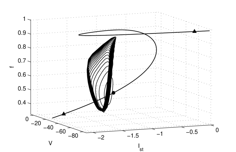
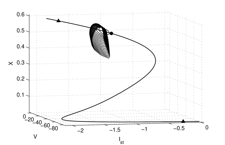
Figure 1: Two projections of limit cycles and of a part of the equilibrium curve (marked by ”$\blacktriangle$”). The Hopf bifurcation point is marked by ”$\bullet$”.

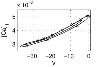
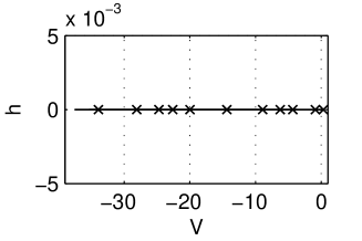
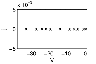
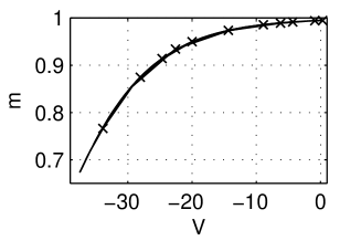
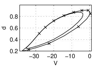
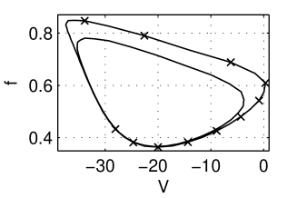
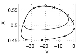
Figure 2: Projections of two limit cycles calculated for $I_{st}$ $=$ $-1.2000465026$ and for $I_{st}$ $=$ $-1.2000183729$ (marked by ”x”) (20 elements, 41 nodes).

8 Numerical results

Based on [30] and on the computer programs for [2] and [3], relations (7), (25), (26), (7) and the algorithm at the end of section 5 furnished the numerical results of this section.

Let $(\lambda^{0},u^{0})$ be the Hopf bifurcation point located during the construction of the equilibrium curve by a continuation procedure in [5]. The solution $(\lambda^{0},\beta^{0},u^{0},g_{r}^{0},g_{i}^{0})$ of (8), calculated in [5], is $\lambda^{0}$ $=$ $-1.0140472901$, $\beta^{0}$ $=$ $0.0162886062$, $u^{0}$ $=$ $(-24.3132508542$, $0.0034641214$, $0.0$, $0.0$, $0.9176777444$, $0.5025242162$, $0.4920204612$, $0.5071561613)$, $g_{r}^{0}$ $=$ $(1.0$, $0.0000468233$, $0.0$, $0.0$, $0.0093195354$, $0.0198748652$, $-0.0072420216$, $0.0001706577)$, $g_{i}^{0}$ $=$ $(0.0$, $0.0000029062$, $0.0$, $0.0$, $-0.0000171311$, $-0.0118192370$, $0.0136415789$, $-0.0017802907)$. (The eigenvalues of the Jacobian matrix $D_{u}F(\lambda^{0},u^{0})$, calculated by the QR algorithm, are $\pm\,0.0162886062\,i$, $-8.8611865338$, $-0.1026761869$, $-0.0647560667$, $-0.0024565181$, $-1.7398266947$, $-0.2049715178$). These data are considered in the step 1 of the algorithm at the end of section 5.

We took $C_{m}=1$, $g_{Na}=23$, $g_{si}=0.09$, $g_{K}=0.282$, $g_{K1}=0.6047$, $g_{Kp}=0.0183$, $G_{b}=0.03921$, $[Na]_{0}=140$, $[Na]_{i}=18$, $[K]_{0}=5.4$, $[K]_{i}=145$, $PR_{NaK}=0.01833$, $E_{b}=-59.87$, $T=310$.

In order to solve (4) numerically by the algorithm at the end of section 5 and by (7), (25), (26), (7), we performed calculations using $\triangle s$ $=$ $1.0$ and 500 iterations in the continuation process. Integrals $\int\limits_{K}f(\tau)\;d\tau$ were calculated using Gauss integration formula with three integration points.

Figure 1 and 2 present some results obtained using 20 elements $K$ (41 nodes) ($N=20$, $J=\{1,\ldots,41\}$ in section 7). The curves of the projections of the limit cycles, on the planes indicates in figure, are plots generated from values calculated in the nodes, corresponding to a fixed value of the parameter.

Two projections of some limit cycles and of a part of the equilibrium curve (marked by ”$\blacktriangle$”) are presented in figure 1. The Hopf bifurcation point is marked by ”$\bullet$”.

In figure 2, there are represented the projections of the plots of two limit cycles calculated for $I_{st}$ $=$ $-1.2000465026$ (iteration 148) and for $I_{st}$ $=$ $-1.2000183729$ (iteration 248, marked by ”x” in figure).

The results obtained are relevant from a biological point of view, pointing to unstable electrical behavior of the modeled system in certain conditions, translated into oscillatory regimes such as early afterdepolarizations ([32]) or self-sustained oscillations ([4]), which may in turn synchronize, resulting in life-threatening arrhythmias: premature ventricular complexes or torsades-de-pointes, degenerating in rapid polymorphic ventricular tacycardia or fibrillation ([26]).

Acknowlegdements: This research was partially supported from grant PNCDI2 61-010 to M-LF by the Romanian Ministry of Education, Research, and Innovation.

References

- [1] G. W. Beeler , H. Reuter, Reconstruction of the action potential of ventricular myocardial fibres, J. Physiol. 268(1977), 177-210.
- [2] C. L. Bichir, A.Georgescu, Approximation of pressure perturbations by FEM, Scientific Bulletin of the Piteşti University, the Mathematics-Informatics Series, 9 (2003), 31-36.
- [3] C. L. Bichir, A numerical study by FEM and FVM of a problem which presents a simple limit point, ROMAI J., 4, 2(2008), 45-56, http://www.romai.ro, http://rj.romai.ro.
- [4] C. L. Bichir, B. Amuzescu, A. Georgescu, M. Popescu, Ghe. Nistor, I. Svab, M. L. Flonta, A. D. Corlan, Stability and self-sustained oscillations in a ventricular cardiomyocyte model, submitted to Interdisciplinary Sciences - Computational Life Sciences, Springer.
- [5] C. L. Bichir, A. Georgescu, B. Amuzescu, Ghe. Nistor, M. Popescu, M. L. Flonta, A. D. Corlan, I. Svab, Limit points and Hopf bifurcation points for a one - parameter dynamical system associated to the Luo - Rudy I model, submitted to Mathematics and its Applications, http://www.mathematics-and-its-applications.com.
- [6] C. Cuvelier, A.Segal, A.A.van Steenhoven, Finite Element Methods and Navier-Stokes Equations, Reidel, Amsterdam, 1986.
- [7] A. Dhooge, W. Govaerts, Yu.A. Kuznetsov, W. Mestrom, A.M. Riet, B. Sautois, MATCONT and CL-MATCONT: Continuation toolboxes in MATLAB, 2006, http://www.matcont.ugent.be/manual.pdf
- [8] E. Doedel, Lecture Notes on Numerical Analysis of Nonlinear Equations, 2007, http://cmvl.cs.concordia.ca/publications/notes.ps.gz, from the Home Page of the AUTO Web Site, http://indy.cs.concordia.ca/auto/.
- [9] A.Georgescu, M.Moroianu, I.Oprea, Bifurcation Theory. Principles and Applications, Applied and Industrial Mathematics Series, 1, University of Piteşti, 1999.
- [10] W. J. Gibb , M. B. Wagner, M. D. Lesh, Effects of simulated potassium blockade on the dynamics of triggered cardiac activity, J. theor. Biol 168(1994), 245-257.
- [11] V.Girault, P.-A.Raviart, Finite Element Approximation of the Navier-Stokes Equations, Springer, Berlin, 1979.
- [12] V.Girault, P.-A.Raviart, Finite Element Methods for Navier-Stokes Equations.Theory and Algorithms, Springer, Berlin, 1986.
- [13] R.Glowinski, Numerical Methods for Nonlinear Variational Problems, Springer, New York, 1984.
- [14] W.J.F. Govaerts, Numerical methods for Bifurcations of Dynamical Equilibria, SIAM, Philadelphia, 2000.
- [15] W. Govaerts, Yu. A. Kuznetsov R. Khoshsiar Ghaziani, H.G.E. Meijer, Cl-MatContM: A toolbox for continuation and bifurcation of cycles of maps, 2008, http://www.matcont.ugent.be/doc-cl-matcontM.pdf
- [16] A. L. Hodgkin, A. F. Huxley, A quantitative description of membrane current and its application to conduction and excitation in nerve, J. Physiol., 117 (1952), 500-544.
- [17] H.B.Keller, Numerical Solution of Bifurcation Eigenvalue Problems, in Applications in Bifurcation Theory, ed. by P.Rabinowitz, Academic, New York, 1977.
- [18] H.B.Keller, Global Homotopies and Newton Methods, in Recent Advances in Numerical Methods, ed. by C. de Boor, G.H.Golub, Academic, New York, 1978.
- [19] Yu. A. Kuznetsov, Elements of Applied Bifurcation Theory, Springer, New York, 1998.
- [20] L. Livshitz, Y. Rudy, Uniqueness and stability of action potential models during rest, pacing, and conduction using problem - solving environment, Biophysical J., 97 (2009), 1265-1276.
- [21] C.H. Luo, Y. Rudy, A model of the ventricular cardiac action potential. Depolarization, repolarization, and their interaction, Circ. Res., 68 (1991), 1501-1526.
- [22] E. Neher, B. Sakmann, Single-channel currents recorded from membrane of denervated frog muscle fibres, Nature, 260 (1976), 799-802.
- [23] D. Noble, Modelling the heart: insights, failures and progress, Bioessays, 24 (2002), 1155-1163.
- [24] D. Noble, From the Hodgkin-Huxley axon to the virtual hear, J. Physiol., 580 (2007), 15-22. Epub 2006 Oct 2005.
- [25] T.S.Parker, L.O.Chua, Practical Numerical Algorithms for Chaotic Systems, Springer, New York, 1989.
- [26] D. Sato, L. H. Xie, A. A. Sovari, D. X. Tran, N. Morita, F. Xie, H. Karagueuzian, A. Garfinkel, J. N. Weiss, Z. Qu , Synchronization of chaotic early afterdepolarizations in the genesis of cardiac arrhythmias, Proc. Natl. Acad. Sci. USA, 106 (2009), 2983-2988. Epub 2009 Feb 2913.
- [27] R. Seydel, Numerical computation of branch points in nonlinear equations, Numer. Math., 33 (1979), 339-352.
- [28] R. Seydel, Nonlinear Computation, invited lecture and paper presented at the Distinguished Plenary Lecture session on Nonlinear Science in the 21st Century, 4th IEEE International Workshops on Cellular Neural Networks and Applications, and Nonlinear Dynamics of Electronic Systems, Sevilla, June, 26, 1996.
- [29] R. Seydel, Practical Bifurcation and Stability Analysis, Springer, New York, 2010.
- [30] C. Taylor, T.G. Hughes, Finite Element Programming of the Navier-Stokes Equations, Pineridge Press, Swansea, U.K., 1981.
- [31] R.Temam, Navier-Stokes equations. Theory and numerical analysis, North-Holland, Amsterdam, 1979.
- [32] D. X, Tran, D. Sato, A. Yochelis, J. N. Weiss, A. Garfinkel, Z. Qu, Bifurcation and chaos in a model of cardiac early afterdepolarizations, Phys. Rev. Lett., 102:258103 (2009). Epub 252009 Jun 258125.
- [33] B. Van der Pol, J. Van der Mark, The heartbeat considered as a relaxation oscillation and an electrical model of the heart, Phil. Mag. (suppl.), 6 (1928), 763-775.