Occupation number-based energy functional for nuclear masses

Abstract

We develop an energy functional with shell-model occupations as the relevant degrees of freedom and compute nuclear masses across the nuclear chart. The functional is based on Hohenberg-Kohn theory with phenomenologically motivated terms. A global fit of the 17-parameter functional to nuclear masses yields a root-mean-square deviation of $\chi=1.31$ MeV. Nuclear radii are computed within a model that employs the resulting occupation numbers.

I Introduction

Nuclear theory seeks to formulate a consistent framework for nuclear structure and reactions. Nuclear density functional theory (DFT) is a particularly useful tool for describing the ground-state properties of nuclei across the nuclear chart Goriely et al. (2002); Bender et al. (2003); Lunney et al. (2003); Stoitsov et al. (2003). This approach is based on the pioneering works of Skyrme Skyrme (1956) and Vautherin Vautherin and Brink (1972); Vautherin (1973) and might theoretically be based on the theorems by Hohenberg and Kohn Hohenberg and Kohn (1964). It has been applied through the self-consistent mean-field computations with density-dependent energy functionals Kohn and Sham (1965). Formally, the energy-density functional results from the Legendre transform of the ground-state energy as a functional of external one-body potentials Lieb (1983). While DFT allows for a simple solution to the quantum many-body problem, the construction of the functional itself poses a challenge Bertsch et al. (2007); Stoitsov et al. (2011). Various efforts aim at constraining the functional from microscopic interactions Stoitsov et al. (2010) or devising a systematic approach Carlsson et al. (2008). In this paper we explore the development of an energy functional that employs shell-model occupations instead of the nuclear density. The minimization of this functional is technically simpler than DFT, and global mass-table fits of the functional require only modest computational resources.

In nuclear physics, energy-density functional theory is a practical tool that is popular because of its computational simplicity and success Bender et al. (2003); Stone and Reinhard (2007). The universality of the functional (i.e., the possibility to study nucleons in external potentials) is seldom used Gandolfi et al. (2011). This distinguishes nuclear DFT from DFT in Coulomb systems and makes alternative formulations worth studying. For computational simplicity, we would like to maintain the framework of an energy functional. However, there is no need to focus only on functionals of the density. The description and interpretation of nuclear systems are often based on shell-model occupation numbers rather than densities Mayer and Jensen (1955). For instance, in nuclear structure one is often as much interested in the occupation of a given shell-model orbital or the isospin-dependence of the effective single-particle energies as in the shape of the density distribution. This approach is natural for shell-model Hamiltonians that are based on single-particle orbitals. The purpose of this paper is to develop a nuclear energy functional constructed in a shell-model framework. We show that an occupation number-based functional can be employed in global mass-table computations and can perform at a competitive level, with a reasonable number of parameters and relatively short computation time.

Many approaches to the nuclear energy-density functional are empirical Dobaczewski et al. (1984); Oliveira et al. (1988); Anguiano et al. (2001); Duguet et al. (2002), but guidance can be found from analytical solutions to simpler models. The complete ground-state energy of a quantum many-body system as a functional of any external potential is available for only a few solvable or weakly interacting systems. Furnstahl and colleagues Furnstahl et al. (2007); Puglia et al. (2003); Bhattacharyya and Furnstahl (2005) derived energy-density functionals for dilute Fermi gases with short-ranged interactions. For Fermi gases in the unitary regime, simple scaling arguments suggest the form of the energy-density functional Carlson et al. (2003); Papenbrock (2006); Bhattacharyya and Papenbrock (2006); Bulgac (2007). We similarly use scaling arguments in the development of our functional.

In recent years, significant progress has been made in developing global nuclear energy-density functionals; see, for example, Refs. Goriely et al. (2009); Kortelainen et al. (2010). The Skyrme-Hartree-Fock-Bogoliubov mass functionals by Goriely et al. Goriely et al. (2009) achieve a least-squares error of about $\chi=0.58$ MeV with 14 parameters fit to nuclei with $N,Z\geq 8$. The 12-parameter UNEDF functionals UNEDFnb and UNEDF0 of Ref. Kortelainen et al. (2010) have a least-squares deviation of $\chi=0.97$ MeV and $\chi=1.46$ MeV, respectively, when fit to a set of 72 even-even nuclei. The fitted functionals, when applied to 520 even-even nuclei of a mass table, yield least-squares deviations of $\chi=1.45$ MeV and $\chi=1.61$ MeV, respectively. The refit Bertsch et al. (2005) of the Skyrme functional Sly4 to even-even nuclei exhibits a root-mean-square deviation of about $\chi=1.7$ MeV. For a recent review on this matter, we refer the reader to Ref. Stone and Reinhard (2007). The work presented here provides an approach based on Hohenberg-Kohn DFT, utilizing degrees of freedom that are natural to the nuclear shell-model, and gives a global description of the nuclear chart for all nuclei with $N,Z\geq 8$.

We emphasize the difference between an energy functional for nuclear masses and a mass formula. Mass formulae, such as the finite-range droplet model (FRDM) Möller et al. (1995) and Duflo-Zuker mass formula Duflo and Zuker (1995), calculate nuclear masses from an assumed nuclear structure. The mass formula by Duflo-Zuker, for instance, computes the binding energy in terms of the shell-model occupations. The occupations are parameters—not variables—and their values are taken from the noninteracting shell-model (with modifications due to deformations). The form of the Duflo-Zuker mass formula is motivated by semiclassical scaling arguments, which ensure that the binding energy scales linearly with the mass number in leading order; see Ref. Mendoza-Temis et al. (2010) for details. The Duflo-Zuker mass formula achieves an impressive root-mean-square deviation of $\chi=0.35$ MeV with 28 fit parameters. In an occupation number-based energy functional, the ground-state energy results from a minimization of a functional, and the occupation numbers are variables that minimize the functional. In other words, the structure of a nucleus results from the minimization of a functional and is not assumed. In our phenomenological construction of an occupation number-based energy functional, we employ several scaling arguments and terms from the Duflo-Zuker mass formula. Recently, the energy functional (in terms of occupation numbers) was constructed for the pairing Hamiltonian Papenbrock and Bhattacharyya (2007); Lacroix and Hupir (2010); Hupin and Lacroix (2011) and the three-level Lipkin model Bertolli and Papenbrock (2008); Lacroix (2009). The analytical insights gained from these simple models also enter the construction of terms for our occupation number-based functional.

This paper is organized as follows. In Sect. II we introduce the form of the energy functional and discuss the relevant terms. In Sects. II.3 and III we provide a statistical analysis of the functional and a description of the minimization routines used. We study the performance of the functional in calculating nuclear ground-state energies and radii in Sect. IV. We conclude with a summary in Sect. V.

II Occupation Number-based Energy Functional

In this section, we introduce the theoretical foundation for functionals based on occupation numbers and discuss the terms that enter the functional.

II.1 Theoretical Basis

We first clarify our work within Hohenberg-Kohn DFT Hohenberg and Kohn (1964). According to Hohenberg and Kohn, for a many-body system with density $\rho$ in an external potential $v$ there exists a functional of the density $\mathcal{F_{HK}}(\rho)$ independent of $v$ such that the ground-state energy is

$$E_{\rm g.s.}=\min\left\{\mathcal{F_{HK}}+\int d^{3}{\bf r}~{}v({\bf r})\rho({\bf r})\right\}.$$ (1)

Here the minimization is performed over all one-body densities $\rho({\bf r})$.

Current nuclear DFT models, such as HFB-17 Goriely et al. (2009), are based on Skyrme forces and employ densities $\rho(\bf{r})$ and currents depending on spatial coordinates. The use of such objects seems a natural choice, particularly in quantum chemistry and condensed matter systems where one is interested in the electronic structure in the presence of ions. For atomic nuclei, however, other representations might also be interesting or more natural, and we consider functionals based on occupations of shell-model orbitals.

To present our concept formally, we consider the ground-state energy $E(\varepsilon_{\alpha})$ of an $A$-body system described by a shell-model Hamiltonian with single-particle energies $\varepsilon_{\alpha}$, $\alpha=1,2,3,\ldots$,

$$\sum_{\alpha}\varepsilon_{\alpha}a_{\alpha}^{\dagger}a_{\alpha}+\hat{V}.$$ (2)

Here, $a_{\alpha}^{\dagger}$ creates a fermion in the shell-model orbital $\alpha$, and $\hat{V}$ is the nuclear interaction. The ground-state energy is a (complicated) function of the single-particle energies, and the occupation number of the orbital with label $\beta$ is

$$n_{\beta}\equiv\frac{\partial}{\partial\varepsilon_{\beta}}E(\varepsilon_{\alpha}).$$ (3)

A Legendre transformation of the function $E(\varepsilon_{\alpha})$ yields the occupation number-based energy functional Lieb (1983)

$$\mathcal{F}(n_{\alpha})=E(\varepsilon_{\alpha}(n_{\beta}))-\sum_{\alpha}n_{\alpha}\varepsilon_{\alpha}(n_{\beta}).$$ (4)

From a technical point of view, the one-body potential—or the mean-field— has been employed as an external potential in DFT. Thus, there is a formal analogy between Hohenberg-Kohn DFT and occupation number functionals. The Hohenberg-Kohn theorems remain valid when we exchange $v(\bf{r})\leftrightarrow\varepsilon_{\alpha}$ and $\rho({\bf r})\leftrightarrow n_{\alpha}$. However, the explicit construction of the occupation number-based energy functional as a Legendre transform is possible only for exactly solvable systems Papenbrock and Bhattacharyya (2007); Bertolli and Papenbrock (2008). In the following section, we employ primarily phenomenological arguments for the terms that enter the functional.

II.2 Form of the Functional

The occupation number-based functional is guided by semiclassical scaling arguments that guarantee nuclear saturation Duflo and Zuker (1995); Mendoza-Temis et al. (2010). In the harmonic oscillator basis, a nucleus of $A$ nucleons has about $A^{1/3}$ occupied shells below the Fermi level, and about $A^{2/3}$ nucleons are in the highest energetic, completely filled shell. We are interested in expressing the functional as a sum of simple functions that depend on occupation numbers. Consider, for example, the energy from a harmonic mean-field potential for the protons. Let $z_{p}$ denote the proton occupation number of the $p$th oscillator shell. The maximum occupation of the $p$th shell is

$$pz_{p}\sim p^{3},$$ (5)

where $\sim$ indicates “scales as.” We use semiclassical arguments to enforce saturation. The total energy of the harmonic mean-field scales as

$$\sum_{p}pz_{p} \simeq \int_{0}^{A^{1/3}}dp~{}p^{3}$$ (6)

$$\sim A^{4/3}.$$ (7)

Thus, the multiplication of such an energy term with a factor of $A^{-1/3}$ ensures saturation, that is, a scaling of the energy with $A$ in leading order. The simple arguments based on filling the major shells of the spherical harmonic oscillator yield incorrect shell closures. As a remedy, we follow Duflo and Zuker Duflo and Zuker (1995) and consider shells where the high-$j$ intruder orbital of the shell $p+1$ enters the shell $p$. Since a single $j$ orbital of the shell $p$ holds on the order of $p$ nucleons—while a major shell holds about $p^{2}$ nucleons—our scaling arguments are unchanged. In the modified shell-model, the resulting shell closures have occupation numbers

$$2,6,14,28,50,82,126,184,....$$ (8)

In what follows, we employ a model space consisting of 15 major shells. The shell $p$ has a dimension $d_{p}=(p+1)(p+2)$, (i.e., it can hold up to $d_{p}$ protons and $d_{p}$ neutrons). We employ suitable factors of $d_{p}$ and $p$ to ensure saturation.

We write the functional as a sum of macroscopic Coulomb and pairing terms plus a microscopic interaction $\mathcal{F}(n,z)$ that depends on the occupations $z_{p}$ of proton shells and $n_{p}$ of neutron shells

$$F(c;n,z)=c_{c}\frac{Z(Z-1)}{A^{1/3}}+c_{P}\frac{\delta}{\sqrt{A}}+\mathcal{F}(c;n,z).$$ (9)

Here, $\delta$ is 1, 0, and -1 for even-even, odd mass, and odd-odd nuclei, respectively, and $Z$ is the charge number. The 17 fit parameters of the full functional are denoted as the shorthand coefficients

$$c\equiv\{c_{1},c_{2},\ldots,c_{11},c_{c},c_{P},c_{s},c_{as},c_{ss},\tilde{c}_{s}\},$$ (10)

while

$$z \equiv \{z_{1},z_{2},\ldots\}$$ (11)

$$n \equiv \{n_{1},n_{2},\ldots\}$$ (12)

denote the occupations of proton and neutron shells, respectively. The microscopic functional $\mathcal{F}(c;n,z)$ has the form

$$\mathcal{F}(c;n,z) = \hbar\omega\bigg{(}V+T_{\rm kin}+I_{\rm 2B}+D$$ (13)

$$+D_{\rm 4B}+\mathcal{T}+M_{\rm 4Bex}+L_{\rm val}\bigg{)}$$

$$+\hbar\tilde{\omega}(\tilde{D}_{\rm 2B}+L+\tilde{L}).$$

Below, we explain the individual terms entering the functional. The functions $\hbar\omega$ and $\hbar\tilde{\omega}$ are

$$\hbar\omega(c_{s},c_{as},c_{ss}) = 1-c_{s}A^{-1/3}$$ (14)

$$-\frac{c_{as}}{1+c_{ss}A^{-1/3}}\frac{T(T+1)}{A^{2}},$$

$$\hbar\tilde{\omega}(\tilde{c}_{s}) = 1+\tilde{c}_{s}A^{-1/3},$$ (15)

and they account for a smooth dependence on the mass and the isospin $T=N-Z$ (with $N$ being the neutron number). Each of the terms of the functional (13) scales at most as $A$. Thus, the functions (14) and (15) include smooth surface corrections. The last term of Eq. (14) provides both a volume- and surface-symmetry correction Danielewicz and Lee (2009); Nikolov et al. (2011).

We now discuss the individual terms of the functional (13). We begin with the volume terms that scale as $A$. These are

$$V \equiv c_{1}A,$$ (16)

$$T_{\rm kin} \equiv c_{2}A^{-1/3}\sum_{p}p(z_{p}+n_{p}),$$ (17)

$$I_{\rm 2B} \equiv c_{3}A^{-1/3}\sum_{p}\bigg{(}\frac{z_{p}(z_{p}-1)}{p}$$ (18)

$$+\frac{n_{p}(n_{p}-1)}{p}+\frac{2n_{p}z_{p}}{p}\bigg{)},$$

$$D \equiv c_{4}\sum_{p}\left(\frac{\sqrt{d_{p}}}{2}-\frac{2}{d_{p}^{3/2}}(z_{p}-d_{p}/2)^{2}\right)$$ (19)

$$\times\sum_{q}\left(\frac{\sqrt{d_{q}}}{2}-\frac{2}{d_{q}^{3/2}}(n_{q}-d_{q}/2)^{2}\right),$$

$$D_{\rm 4B} \equiv c_{6}\sum_{p}\frac{z_{p}(d_{p}-z_{p})n_{p}(d_{p}-n_{p})}{d_{p}^{3}},$$ (20)

$$L \equiv c_{7}\sum_{p}\bigg{(}\sqrt{(z_{p}+\varepsilon)(n_{p}+1)}$$ (21)

$$+\sqrt{(n_{p}+\varepsilon)(z_{p}+1)}\bigg{)},$$

$$\mathcal{T} \equiv c_{9}\sum_{p}\sqrt{(n_{p}-z_{p})^{2}+\varepsilon^{2}}.$$ (22)

Note that $\varepsilon=10^{-3}$ is a regularization parameter in Eqs. (16)-(22), to ensure differentiability. The term $V$ of Eq. (16) is a smooth volume term and accounts for the bulk energy. The term $T_{\rm kin}$ of Eq. (17) contains a contribution of the single-particle kinetic energies. This term exhibits shell effects and thereby corrects the smooth behavior of the volume term $V$. Effects of two-body interactions are captured by the terms beginning with Eq. (18). The two-body term $I_{\rm 2B}$ is motivated by the monopole Hamiltonian in the mass formula by Duflo and Zuker Duflo and Zuker (1995). Here, the fermionic nature in the proton-proton and neutron-neutron interaction is evident.

The term $D$ of Eq. (19) is technically a two-, three- and four-body interaction and serves to include deformation effects. The form of this term has a linear onset for almost-empty and almost-filled shells and assumes its maximum at mid-shell with half-filled occupations. In practice, this term behaves similar to the function $\min(n_{p},d_{p}-n_{p})$ but does not suffer from discontinuity and lack of differentiability. Similarly, the four-body term $D_{\rm 4B}$ of Eq. (20) also accounts for deformation effects.

The term of Eq. (21) is motivated by the analytical results in Refs. Bertolli and Papenbrock (2008); Papenbrock and Bhattacharyya (2007). For a two-level system with interactions between the levels, the minimum energy results in a fractional occupation of the higher level due to a square root singularity in the functional. Such square root terms are present in the functional of the three-level Lipkin model Bertolli and Papenbrock (2008) and the pairing Hamiltonian Papenbrock and Bhattacharyya (2007); Lacroix and Hupir (2010). The inclusion of these analytically motivated terms considerably improves the functional’s reproduction of experimental energies.

The term $\mathcal{T}$ of Eq. (22) is an isospin term and includes the isospin contributions of individual orbitals. Not surprisingly, Eq. (22) turns out to be relevant for the accurate descriptions of nuclei far from the $N=Z$ line. For computational purposes Eq. (22) is written in square roots rather than absolute values. For $|n_{p}-z_{p}|\gg\varepsilon$ we have $\sqrt{(n_{p}-z_{p})^{2}+\varepsilon^{2}}\simeq|n_{p}-z_{p}|$, and this term is thus practically a differentiable approximation of the absolute value.

The volume terms of Eqs. (16) to (22) also have surface corrections due to the discrete sums. However, we also need to include surface corrections independent of the volume terms. Technically, surface terms scale as $A^{2/3}$. We employ

$$\tilde{D}_{\rm 2B} \equiv c_{5}\sum_{p}\left(\frac{z_{p}(d_{p}-z_{p})}{d_{p}^{3/2}}+\frac{n_{p}(d_{p}-n_{p})}{d_{p}^{3/2}}\right),$$ (23)

$$\tilde{L} \equiv c_{8}A^{-2/3}\sum_{p}\left(z_{p}\sqrt{z_{p}+1}+n_{p}\sqrt{n_{p}+1}\right),$$ (24)

$$M_{\rm 4Bex} \equiv c_{10}\sum_{p}\frac{1}{p^{23}}\bigg{[}(z_{p}(z_{p}-1)(z_{p}-2)(z_{p}-3))^{3}$$ (25)

$$+(n_{p}(n_{p}-1)(n_{p}-2)(n_{p}-3))^{3}\bigg{]},$$

$$L_{\rm val} \equiv c_{11}\bigg{(}\sqrt{(d_{f}-n_{f})n_{f+1}+\varepsilon^{2}}$$ (26)

$$+\sqrt{(d_{f}-z_{f})z_{f+1}+\varepsilon^{2}}\bigg{)}.$$

The term $\tilde{D}_{\rm 2B}$ of Eq. (23) accounts for microscopic pairing contributions. Its form is motivated by Talmi’s seniority model Talmi (1962), again with a maximum contribution at mid-shell as with the volume term of Eq. (19). Likewise, the term $\tilde{L}$ of Eq. (24) is a surface correction term to the volume term (21).

The term in Eq. (25) accounts for higher-order effects and resulted from an efficient scheme to identify relevant contributions that we describe in Sect. II.4. The powers of $p$ ensure the desired $A^{2/3}$ scaling.

The term $L_{\rm val}$ of Eq. (26) is unique as it involves only the highest occupied shell ($p=f$) in the noninteracting shell-model; that is, it treats the shell immediately below (with occupation $n_{f}$) and above (with occupation $n_{f+1}$) the Fermi surface. In the naive shell-model, these shells contain about $A^{2/3}$ nucleons, and $L_{\rm val}$ thus is a surface term. This term accounts for energy from particle-hole excitations and turns out to be useful. We note that the forms of Eqs. (16)-(26) are symmetric about exchange of protons and neutrons, $z_{p}\leftrightarrow n_{p}$. Therefore, the only isospin breaking term of our functional is the Coulomb term of Eq. (9).

II.3 Numerical Implementation

We consider one of the $N_{\rm pts}$ nuclei of the nuclear chart and label it by $i$. This nucleus has neutron number $N_{i}$ and proton number $Z_{i}$. The minimization of the functional (9) with respect to the occupations $n,z$ yields the ground-state energy

$$E_{i}(c;n^{*}(c),z^{*}(c)) = \min_{n,z\in\mathcal{D}_{i}}F(c;n,z).$$ (27)

We refer to this minimization as the lower-level optimization. In Eq. (27), $n^{*}(c),z^{*}(c)$ denote the optimal occupation numbers (we suppress that they depend on the label $i$) and are taken from the domain

$$\mathcal{D}_{i}=\bigg{\{}(n,z):$$

$$\sum_{p}n_{p}=N_{i};\sum_{p}z_{p}=Z_{i};0\leq n_{p},z_{p}\leq d_{p}\bigg{\}}.$$

From a mathematical point of view, we deal with an optimization problem that includes linear equality constraints and bound constraints. The functional (9) is nonlinear but twice continuously differentiable in the occupation numbers $n,z$ over the domain $\mathcal{D}$. Furthermore, given the coefficients $c$, we have algebraic derivatives of $F$ with respect to $n,z$ and can use these to solve each lower-level problem. We used the sequential quadratic programming (SQP) routine FFSQP Zhou et al. (1997) to solve the constrained optimization problem (27).

We provided FFSQP with analytical expressions for the gradient of $F$ with respect to $n$ and $z$. These gradients are used by FFSQP to build second-order approximations of the objective while remaining within the constrained domain $\mathcal{D}_{i}$. The value of $F$ is iteratively reduced until further local decreases would be infeasible with respect to $\mathcal{D}_{i}$. This provides a local minimum in the neighborhood of our starting point at the naive level-filling. We found that the additional effort of employing the derivatives with respect to the occupation numbers provided significant advantages, in terms of speed and stability, over other optimization routines such as COBYLA Powell (1994), that do not require derivatives to be available.

As a starting point, we provide FFSQP with the occupation numbers $n$ and $z$ corresponding to the naive level filling, which are feasible for the domain $\mathcal{D}_{i}$. In practice, a local solution is found within about a dozen function and gradient calls.

The fit coefficients $c$ are then determined by minimizing the sum of squared residuals

$$\chi^{2}(c)=\frac{1}{N_{\rm pts}}\sum_{i=1}^{N_{\rm pts}}\left[E_{i}(c;n^{*}(c),z^{*}(c))-E_{i}^{\rm exp}\right]^{2}$$ (29)

as a function of $c$. Here, $E_{i}^{\rm exp}$ denotes the measured ground-state energy of the nucleus $i$. Technically, we deal with a multi-level optimization problem because each of the theoretical energies $E_{i}$ is a solution of a lower-level optimization of the functional (9) over the occupation numbers $n$ and $z$. Obtaining the occupations from an optimization is in contrast to the mass formula Duflo and Zuker (1995), where occupations are fixed and input by hand. We refer to the optimization of the coefficients $c$ as the upper-level optimization problem. This problem is solved with the program POUNDerS (Practical Optimization Using No Derivatives for sums of Squares), and details are presented in Sect. III.

Note the computational complexity present in the minimization of the chi-square (29). For each of the $N_{\rm pts}$ nuclei we must perform a lower-level minimization of the functional to determine occupation numbers that minimize the functional and yield the ground-state energy $E_{i}$. The occupation numbers resulting from this lower-level optimization can be very sensitive to the coefficients $c$ of the functional, which in turn are determined in the upper-level chi-square minimization. To reduce the wall clock time of each $\chi^{2}$ evaluation, we can perform the lower-level minimizations in parallel, using as many as $N_{\rm pts}$ processors. Further details of the $\chi^{2}$ minimization are presented in Sect. III.

The computation of ground-state energies via the functional (9) with coupled minimizations differs considerably from the uncoupled case. If the proton and neutron occupations are kept fixed to the naive level filling, Eq. (9) becomes a mass formula. Performing a chi-square fit with this fixed filling yields coefficients $c$ that can then be used when minimizing the functional with respect to occupations (that is, the lower-level minimization is done independently of the upper-level minimization). The resulting error, $\chi=3.38$ MeV, is one order of magnitude larger than the residual error of the mass formula by Duflo and Zuker Duflo and Zuker (1995). When including the lower-level optimization in the chi-square fit (and hence dealing with a multi-level optimization), we obtain a considerably reduced $\chi=1.31$ MeV.

II.4 Determination of Relevant Terms

Unfortunately, there is no recipe available for the construction of the occupation-number-based energy functional, and the reader may wonder how we arrived at the particular form (13) of the functional. As described in Sect. II.2, the guiding principles are saturation, mean-field arguments, and insights from analytically solvable systems. However, these arguments do not fully constrain the functional, and we need a more systematic approach to identify terms that should enter into the functional.

Bertsch et al. Bertsch et al. (2005) employed the singular value decomposition and studied the statistical importance of various linear combinations of terms that enter the functional. This method identifies the relative importance of possible combinations of terms and truncates search directions that are flat in the parameter space. Along these ideas, we employ a method that chooses new functional terms based on their correlation to terms already present. New terms are chosen to provide a relatively independent “search direction” in the parameter space of the coefficients $c$ in which the $\chi^{2}$ of Eq. (29) is minimized. This approach is presented in detail in Subsect. II.4.1.

In mass formulae, the addition of new terms (and new fitting parameters) yields a chi-square that is a monotone decreasing function with the number of fit parameters. For a functional, however, matters are different. Here, the addition of a new term to the functional guarantees a lowered chi-square only if the term has a perturbatively small effect. This point is discussed in Subsect. II.4.2.

II.4.1 Correlation Test

We first describe our method for selecting new terms to be included in the functional, beyond those strongly motivated by scaling arguments, mean-field arguments, and solutions to simple analytic systems. We seek a systematic method for determining new terms that will provide further insight into the physical system and decrease the overall chi-square.

Consider the addition of a term $c_{f}f$, with new fit parameter $c_{f}$, to the functional

$$F_{0}(c;n,z)=$$ (30)

$$c_{c}\frac{Z(Z-1)}{A^{1/3}}+c_{P}\frac{\delta}{\sqrt{A}}+\sum_{\alpha=1}^{M}c_{\alpha}f_{\alpha}(n^{*}(c),z^{*}(c)).$$

This functional contains $M$ terms depending on occupation numbers, $n^{*},z^{*}$ denoting the occupation numbers that minimize $F_{0}$ for a given nucleus. The occupation numbers depend on the nucleus $i$ under consideration, but we suppress this dependency. One can expect that the addition of the term $c_{f}f$ to $F_{0}$ will be useful in lowering the chi-square only when it is independent of the $M$ terms already included in the functional.

For identification of a new search direction we compute the correlation coefficient

$$R_{f_{\alpha},f} = \frac{\mbox{cov}(f_{\alpha},f)}{s_{f_{\alpha}}s_{f}}.$$ (31)

Here the covariance is

$$\mbox{cov}(f_{\alpha},f)=\langle f_{\alpha}f\rangle-\langle f_{\alpha}\rangle\langle f\rangle,$$ (32)

and the average $\langle\cdot\rangle$ is computed with respect to the $N_{\rm pts}$ nuclei of the nuclear chart. Similarly, the standard deviations are

$$s_{f}=\sqrt{\langle f^{2}\rangle-\langle f\rangle^{2}}\mbox{ and }s_{f_{\alpha}}=\sqrt{\langle{f_{\alpha}}^{2}\rangle-\langle{f_{\alpha}}\rangle^{2}}.$$ (33)

In the computation of the averages, the terms $f$ and $f_{\alpha}$ are evaluated at the occupations $(n^{*}(c),z^{*}(c))$ that minimize Eq. (30). Here $(n^{*}(c),z^{*}(c))$ depend on the coefficients $c$ that minimize the $\chi^{2}$ based on the energies in Eq. (30). We note that the correlation coefficient is independent of the size of the coefficient $c_{f}$ of the new term under consideration, though dependent on the other fit coefficients $c$ through the optimal occupations $(n^{*}(c),z^{*}(c))$. Should the correlation be sufficiently low for all included terms, the new term $c_{f}f$ becomes a candidate and is tested for its performance in lowering the $\chi$ value.

This approach allows us to probe many different forms of functional terms and then scan through several hundred iterations without the time-consuming and computationally expensive aspects of performing a full minimization of the chi-square for each new term under question. In this way, we systematically grow the functional term by term. We started from an initial base of about 350 different terms and found that only 18 of them were weakly correlated to the existing terms and had the potential to significantly decrease the least-squares error. Of these 18 terms, 15 were seen to be simply higher-order corrections of three primary forms. We further reduced the set of possible terms through physical arguments and preliminary fits. This approach showed Eq. (22) to be the best choice for lowering our least-squares deviation. Equations (25) and (26) were determined similarly, from very large sets of possible terms. In this way we successfully lowered the functional’s least-squares error to a meaningful $\chi=1.31$ MeV with 17 fit parameters.

II.4.2 Perturbative Test

Assume again that our functional $F_{0}$ is as in Eq. (30), and that we consider the addition of a new term $c_{f}f$ (with the new fit coefficient $c_{f}$ taken to be the mean value of the currently determined fit coefficients, where there are no statistical outliers). We will consider the general case where the new term $f$ depends also on the fit coefficients $c$ of $F_{0}$. In what follows, we consider a single nucleus with the ground-state energy

$$E_{0}\equiv F_{0}(c;n^{*},z^{*})$$ (34)

obtained from the functional $F_{0}$. Let us assume that

$$f(c;n^{*},z^{*})\ll E_{0}.$$ (35)

Thus, the new term is perturbatively small (assuming that the new fit coefficient $c_{f}$ is of “natural” order one). Furthermore, we make the assumption that $f$ is of “natural” size and perturbatively small in a neighborhood of $(n^{*},z^{*})$ (i.e., its derivatives in this neighborhood are of the same order as $f$). We consider $F=F_{0}+c_{\rm new}f_{\rm new}$, and it is clear that the minimum of $F$ will be found at some new occupations $n^{*}+\delta n,z^{*}+\delta z$ with corrections $\delta n$ and $\delta z$ that are much smaller than $n^{*}$ and $z^{*}$, respectively. We expand

$$\min_{n,z\in\mathcal{D}_{i}}\Big{(}F_{0}(c;n,z)+c_{f}f(c;n,z)\Big{)}$$ (36)

$$= F_{0}(c;n^{*}+\delta n,z^{*}+\delta z)+c_{f}f(c;n^{*}+\delta n,z^{*}+\delta z)$$

$$\approx F_{0}(c;n^{*},z^{*})+c_{f}f(c;n^{*},z^{*})$$

$$+\sum_{p}\frac{\partial F_{0}}{\partial n_{p}}\bigg{|}_{n^{*},z^{*}}\delta n_{p}+\sum_{p}\frac{\partial F_{0}}{\partial z_{p}}\bigg{|}_{n^{*},z^{*}}\delta z_{p}$$

$$+c_{f}\sum_{p}\frac{\partial f}{\partial n_{p}}\bigg{|}_{n^{*},z^{*}}\delta n_{p}+c_{f}\sum_{p}\frac{\partial f}{\partial z_{p}}\bigg{|}_{n^{*},z^{*}}\delta z_{p}$$

$$\approx F_{0}(c;n^{*},z^{*})+c_{f}f(c;n^{*},z^{*}),$$

and the approximation is due to our limitation to first-order corrections. Note that we have expanded to first-order in smallness, eliminating terms that go as derivatives of $f$ since $|f^{\prime}\delta n|\ll|F_{0}|$ and $|f^{\prime}\delta p|\ll|F_{0}|$. The derivatives of the functional $F_{0}$ with respect to the occupation numbers vanish at the optimum occupation numbers $(n^{*},z^{*})$, where it is understood that the variation is only with respect to those occupation numbers that are not at any of the boundaries (i.e., those occupation numbers for which $n^{*}_{j}\neq 0$ or $d_{j}$ and $z^{*}_{j}\neq 0$ or $d_{j}$), and that the variation fulfills the equality constraints. Technically speaking, these are the reduced derivatives Mielke and Theil (2004). Thus, in leading order of perturbation theory, the functional is simply a mass formula (as it is evaluated at the leading-order occupations), and the chi-square fit cannot yield an increased root-mean-square error for the ground-state energies. In the worst case, $c_{f}=0$ will result from the fit. Thus, only the addition of terms to the functional that cause perturbatively small changes to the occupation numbers are expected to result in a decreased chi-square.

For quickly evaluating a new candidate term $f$ to be added to the functional, we begin by treating the full functional as a mass formula. That is, we freeze the proton and neutron occupations at the optimal values determined prior to the addition of the new term and approximate the ground-state energy in the presence of the new term as

$$E_{i}(c;n^{*},z^{*})\approx F(c;n^{*},z^{*})+c_{f}f_{\rm new}(n^{*},z^{*}).$$ (37)

We evaluate the energy (37) for each nucleus $i$, perform a $\chi^{2}$ minimization of the resulting mass formula (37), and obtain a new set of test coefficients, $c_{\rm test}$. Using these coefficients we recalculate the occupations $n^{*}_{\rm test},z^{*}_{\rm test}$ and the ground-state energies

$$E_{i}(c_{\rm test};n^{*}_{\rm test},z^{*}_{\rm test})=$$ (38)

$$\min_{n,z\in\mathcal{D}_{i}}\Big{(}F(c_{\rm test};n,z)+c_{f}f(c_{\rm test};n,z)\Big{)}$$

that minimize the functional. The computation of the corrections $(\delta n,\delta z)\approx(n^{*}_{\rm test}-n^{*},z^{*}_{\rm test}-z^{*})$ to the occupation numbers shows whether the new term is perturbative in character and can thus be expected to lower the chi-square.

II.5 Model for Nuclear Radii

In DFT the radius $r$ of a nucleus is computed from the density $\rho({\bf r})$ as

$$\langle r^{2}\rangle=\frac{1}{A}\int d{\bf r}^{3}~{}{\bf r}^{2}\rho({\bf r}).$$ (39)

In constructing the functional we employed a harmonic oscillator basis for the shell-model and the scaling arguments. Consequently, we also employ it for the computation of $\langle r^{2}\rangle$. The expectation value of the radius squared in the harmonic oscillator shell with principal quantum number $\nu$ and angular momentum $\lambda$ is

$$\langle\nu\lambda|r^{2}|\nu\lambda\rangle=\ell^{2}(2\nu+\lambda+3/2).$$ (40)

Here, $\ell$ is the oscillator length and is set to $\sqrt{492.5A^{1/3}}$ fm, and $m$ is the mass of the proton. We use $p=2\nu+\lambda$ and thus find for the expectation value of the charge radius squared

$$\langle r^{2}\rangle=\frac{\ell^{2}}{Z}\sum_{p}z_{p}(p+3/2).$$ (41)

In computing charge radii, we must account for the finite size of the nucleons Friar et al. (1997),

$$\langle r_{ch}^{2}\rangle=\langle r_{p}^{2}\rangle+\langle r_{ch,p}^{2}\rangle+\frac{N}{Z}\langle r_{ch,n}^{2}\rangle.$$ (42)

Here, the proton and neutron charge radii are $\sqrt{\langle r_{ch,p}^{2}\rangle}=0.877$ fm, $\langle r_{ch,n}^{2}\rangle=-0.1161$ fm², respectively.

We follow Ref. Duflo (1994) and compute the charge radius within the following model:

$$\mathcal{V}=v_{1}+v_{2}r^{3}+v_{3}\frac{N-Z}{r}+v_{4}\frac{(N-Z)^{2}}{r^{3}}$$ (43)

$$r_{\rm fit}(v;z)=v_{5}\mathcal{V}^{1/3}+v_{6}.$$ (44)

Here $r=\sqrt{\langle r_{ch}^{3}\rangle}$, and the coefficients $v$ parameterize the model. We perform a $\chi^{2}$ fit of the radii to determine the coefficients $v\equiv(v_{1},\ldots,v_{6})$ in Eqs. (43) and (44), whereby we minimize

$$\chi_{r}^{2}(v)=\frac{1}{N_{\rm pts}}\sum_{i=1}^{N_{\rm pts}}\left(r_{{\rm fit},i}(v;z)-r_{i}^{\rm exp}\right)^{2}.$$ (45)

III Minimization of the Functional

The POUNDerS algorithm was developed for nonlinear least-squares problems where the derivatives of the residuals are unavailable. A summary of the algorithm in the context of DFT can be found in Kortelainen et al. (2010).

For fixed $n$ and $z$, the derivatives $\nabla_{c}E_{i}^{\rm th}(c;n,z)$ are known and continuous except when $c_{ss}=-A^{1/3}$ for some nucleus; see Eq. (14). However, the form of the nonlinear lower-level minimization in Eq. (27) does not satisfy standard regularity conditions that would ensure existence and continuity of the derivatives $\frac{\partial n^{*}(c)}{\partial c_{j}}$ and $\frac{\partial z^{*}(c)}{\partial c_{j}}$ (see, e.g., Robinson (1980)). Thus, unavailability of the residual derivatives in our case comes from the dependence of the optimal occupation numbers $n^{*},z^{*}$ on the coefficients $c$.

From a theoretical standpoint POUNDerS requires continuously differentiable residuals. For this functional, however, we found that a smooth model-based method accounting for the problem structure yielded better coefficients in fewer simulations than do optimization algorithms that can explicitly treat the nonsmoothness. A similar result was found for many of the piecewise smooth problems in Moré and Wild (2009).

To minimize Eq. (29), the POUNDerS used in Kortelainen et al. (2010) was modified to account for known partial derivatives with respect to some of the coefficients. The optimal occupations $\{n^{*}(c)\},\{z^{*}(c)\}$ are independent of the three coefficients ($c_{c},c_{P},c_{1}$) because the corresponding terms in the functional Eq. (13) do not involve $n,z$. Hence we can algebraically compute the (continuous) derivatives

$$\frac{\partial E_{i}^{\rm th}}{\partial c_{j}},\,\frac{\partial^{2}E_{i}^{\rm th}}{\partial c_{j}\partial c_{k}},\qquad j,k\in\{c,P,1\}.$$ (46)

The unavailability of derivatives makes optimization significantly more challenging. Over the course of the optimization, POUNDerS effectively builds up coarse approximations to first- and second-order derivatives of the residuals by interpolating the residuals at previously evaluated coefficient values. Knowing the residual derivatives of 3 of the 17 coefficients effectively lowers the dimension of the difficult derivative-free optimization problem, resulting in fewer evaluations of $\chi^{2}$.

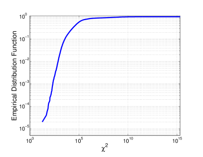
Figure 1: (Color online) $\log-\log$ empirical cumulative distribution function showing the probability of randomly finding a value below the given $\chi^{2}$ value in the hypercube $[-1,1]^{17}$.

To guard against the effects of multiple local $\chi^{2}$ minimizers and discontinuities of the computed energies, we found that a sufficient strategy was periodic restarting of POUNDerS in neighborhoods of mild size. This allows the local algorithm to occasionally look beyond the smaller neighborhood it has focused on. While it is impossible to guarantee that $\chi^{2}$ has been globally minimized, the local solution reported in the next section is significantly better than the $\chi^{2}$ values found for other coefficients. Based on $50,000$ $c$ values uniformly drawn from the hypercube $[-1,1]^{17}$, Fig. 1 shows that roughly $0.01\%$ of $c$ have $\chi^{2}\leq 10^{2}$ and roughly $50\%$ have $\chi^{2}\geq 10^{5}$. This shows that by taking into account the structure of $\chi^{2}$ and the availability of some derivatives, with POUNDerS we were able to find a proverbial “needle in a haystack” with $\chi\approx 1$.

IV Results

We now analyze the results of the functional based on coefficients $c$ determined by the $\chi^{2}$ fit (29) of the energy calculations to experimental data.

IV.1 Energy

We fit our functional to a set of 2,049 nuclei from the 2003 atomic data evaluation Audi et al. (2003) whose uncertainty in the binding energy is below 200 keV. The resulting fit produces a least-squares error of $\chi=1.31$ MeV, and the fit coefficients in units of MeV are

$$c_{c} = -0.619948,$$

$$c_{p} = 11.170908,$$

$$c_{s} = 0.891816,$$

$$c_{as} = 7.434098,$$

$$c_{ss} = 0.397623,$$

$$c_{2} = 23.174559,$$

$$c_{3} = 0.233345,$$

$$c_{4} = 0.493533,$$

$$c_{5} = -10.678202,$$

$$c_{6} = -0.353447,$$

$$c_{1} = -7.672829,$$

$$\tilde{c}_{s} = -0.429029,$$

$$c_{8} = 7.333364,$$

$$c_{7} = 0.112605,$$

$$c_{9} = 0.382828,$$

$$c_{10} = -4.107110,$$

$$c_{11} = 1.383515.$$

Our root-mean-square deviation is competitive with current Skryme force-based functionals Kortelainen et al. (2010). While the current least-squares deviation is greater than the best achieved by a mean-field based functional Goriely et al. (2009), we provide a novel mass functional that uses the orbital occupations of nucleons as the relevant degrees of freedom.

Figure 2 shows an $N$ vs. $Z$ chart of the fit nuclei with color representing the difference $E^{\rm th}-E^{\rm exp}$ between the energies computed from the functional and the experimental data for the 2,049 nuclei employed in the fit. The differences are a smooth function of the neutron and proton numbers. Figures 3 and 4 display the energy differences as functions of $N$ and $Z$. There are still systematic deviations associated with shell oscillations. Recall that the shell closures are input to our functional through the choice of the single-particle degrees of freedom. Thus, the shell oscillations reflect smaller deficiencies associated with the description of nuclear deformation.

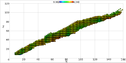
Figure 2: (Color online) Chart of 2,049 well-measured nuclei from the 2003 atomic data evaluation in Ref. Audi et al. (2003), color showing the difference $E^{\rm th}-E^{\rm exp}$ between the calculated energy and experimental energy. The energy difference exhibits a smooth behavior across the whole chart. Some overbinding is seen in the area of very heavy nuclei and tin isotopes. Color ranges from -9.962 MeV (blue) to 4.340 MeV (red).

Figure 3: Energy difference $E^{\rm th}-E^{\rm exp}$ as a function of $N$ for the same nuclei as in Fig. 2. The small oscillations around zero indicate a good description of nuclear shell structure.

Figure 4: Energy difference $E^{\rm th}-E^{\rm exp}$ as a function of $Z$ for the same nuclei as in Fig. 2. The small oscillations around zero indicate a good description of nuclear shell structure.

To test the extrapolation properties of our functional, we fit the functional to a smaller set of 1,837 nuclei taken from the 1993 atomic evaluation data set Audi and Wapstra (1993). For this data set, the root-mean-square error is $\chi=1.38$ MeV. This least-squares deviation is close to that from a fit to the larger set of 2,049 nuclei, and the deviations are again smooth across the nuclear chart. Employing the functional from the fit to the 1993 data set, we compute the ground-state energies of all 2,049 nuclei and find a root-mean-square deviation of $\chi=1.34$ MeV. Thus, the functional has good extrapolation properties.

To further test the functional’s predictive power, we use the coefficients $c$ from the fit to the 1993 data set ($\chi=1.38$ MeV) and the coefficients from the fit to the 2,049 nuclei ($\chi=1.31$ MeV) and compute the binding energies of 2,149 nuclei in the complete 2003 nuclear data set. The functional fit to the 1993 data set yields $\chi=1.40$ MeV, and the functional from a fit to the 2,049 nuclei yields $\chi=1.38$ MeV. These values are close to $\chi=1.37$ MeV that results from a fit of the functional to the full 2003 data set. Thus, the extrapolation properties of the functional are quite good. Table 1 summarizes the details of how our functional extrapolates from data set to data set. Figure 5 shows the differences between theoretical and experimental ground-state energies across the chart of nuclei employed for the extrapolation.

Table 1: Root-mean-square deviations of binding energies resulting from a global fit of the functional and from extrapolation to larger data sets. Data set A consists of all nuclei of the 1993 mass evaluation Audi and Wapstra (1993), data set C consists of all nuclei of the 2003 mass evaluation Audi et al. (2003), and data set B is a subset of data set C consisting of well-measured nuclei whose uncertainty in the mass is below 200 keV. The number of nuclei in each data set is denoted by $N_{\rm pts}$.

Data		$\chi$ (MeV)
Set			Extrapolation to
	$N_{\rm pts}$	Fit	Data Set B	Data Set C
A	1837	1.38	1.34	1.40
B	2049	1.31	–	1.38
C	2149	1.37	–	–

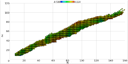
Figure 5: (Color online) Energy difference $E^{\rm th}-E^{\rm exp}$ between theoretical and experimental results for the functional that is fit to the 1993 data set and applied to the subset B of well-measured nuclei of the 2003 data set. The deviations are smooth across the nuclear chart and consistent with Fig. 2. Color ranges from -8.530 MeV (blue) to 4.114 MeV (red).

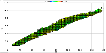
Figure 6: (Color online) Energy difference $E^{\rm th}-E^{\rm exp}$ between theoretical and experimental results for the functional fit to the 1993 data set and applied to the 2003 data set. The deviations are smooth across the nuclear chart and consistent with Fig. 2. Color ranges from -9.263 MeV (blue) to 6.183 MeV (red).

IV.2 Radii

We now turn to the results for nuclear charge radii. We fit our six-parameter model (44) for the charge radii to the experimental data of 772 nuclei from Ref. Angeli (2004) and obtain a least-squares deviation of $\chi_{r}=0.047$ fm. The resulting fit coefficients (with units of fm) are

$$v_{1} = 11.004005,$$

$$v_{2} = 2.000870,$$

$$v_{3} = -3.248108,$$

$$v_{4} = -0.279495,$$

$$v_{5} = 0.775617,$$

$$v_{6} = -0.557746.$$

Note that the data set contains both spherical and deformed nuclei. Figure 7 shows the difference between the calculated and experimental radii. For a comparison, note that Duflo and Zuker state a least-squares error of about $\chi_{r}\simeq 0.01$ fm for the charge radii of spherical nuclei Duflo (1994). Radii from Skyrme functionals exhibit a root-mean-square deviation of about 0.025 fm Stone and Reinhard (2007). Figure 8 shows the difference between computed and experimental charge radii as a function of neutron number. The outliers seen in Fig. 8 correspond to isotopic chain of Tb and the elements Rb, Sr and Zr with neutrons $N=60-62$.

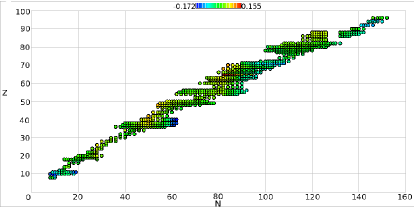
Figure 7: (Color online) Difference between experimental and theoretical charge radii for the set of 772 nuclei from Ref. Angeli (2004). Color ranges from -0.172 fm (blue) to 0.155 fm (red).

Figure 8: Chart of difference between calculated and experimental charge radii for 772 nuclei as a function of $N$. Lines connect isotopes.

Let us also study the extrapolation properties of our mass model. We fit the model (44) to the charge radii on a subset of 494 nuclei (taken from Ref. Angeli (2004)) chosen near the valley of stability. This yields a least-squares error of $\chi_{r}=0.046$ fm. When using this model to compute the charge radii on the full set of 772 charge radii, we find a slightly increased $\chi_{r}=0.048$ fm, indicating that the extrapolation is successful.

For each nucleus, the occupation numbers enter the computation of the charge radius. We thus need to understand how our model for the charge radius depends on the functional employed for the computation of binding energies; in other words, its dependence on the coefficients $c$. A sensitivity analysis of our fit to binding energies provides us with a confidence interval for each of the coefficients $c$. We take a randomly chosen sample of five sets of coefficients $\{c_{1},\dots,c_{5}\}$ within the confidence interval and recompute the structure (i.e., the occupation numbers) and the binding energies. The resulting least-squares deviations for binding energy range from $\chi=1.34$ MeV to $1.78$ MeV. Subsequently, we compute the charge radii for the nuclei of interest (without refitting the coefficients $v$ of our model for the radii). If we refit the coefficients $v$ of our mass model and adjust them to the change in the coefficients $c$ of the energy functional, the least-squares error for the radii changes by at most 4%. Thus, we find the surprising result that the model for radii is relatively independent of the functional’s fit coefficients $c$.

V Summary

We constructed an occupation number-based energy functional for the calculation of nuclear binding energies across the nuclear chart. The relevant degrees of freedom for the functional are the proton and neutron orbital occupations in the shell-model. A global fit of a 17-parameter functional to nuclear masses yields a least-squares deviation of $\chi=1.31$ MeV for the binding energies, and a simple six-parameter model for the charge radii yields a root-mean-square deviation of $\chi_{r}=0.047$ fm. The functional has good extrapolation properties, evident from the application of the functional fit to data from the 1993 atomic mass evaluation to the nuclei of the 2003 atomic mass evaluation. The form of the functional is guided by scaling arguments and by results from analytically solvable models. Isospin and surface correction terms in the functional proved to be important. These terms were determined by a systematic investigation of correlations among possible terms for the functional and by an analysis of their perturbative behavior. Additional terms, and therefore lower least-squares deviations, may be obtained through further use of this method, as well as greater investigation of the microscopic contributions of higher-order effects in surface and radial terms.