Pattern formation in auxin flux

Abstract

The plant hormone auxin is fundamental for plant growth, and its spatial distribution in plant tissues is critical for plant morphogenesis. We consider a leading model of the polar auxin flux, and study in full detail the stability of the possible equilibrium configurations. We show that the critical states of the auxin transport process are composed of basic building blocks, which are isolated in a background of auxin depleted cells, and are not geometrically regular in general. The same model was considered recently through a continuous limit and a coupling to the von Karman equations, to model the interplay of biochemistry and mechanics during plant growth. Our conclusions might be of interest in this setting, since, for example, we establish the existence of Lyapunov functions for the auxin flux, proving in this way the convergence of pure transport processes toward the set of critical configurations.

1 Introduction

The plant hormone auxin plays a fundamental role in plant development (Reinhardt et al., 2000, 2003), and its spatial distribution in plants tissues is critical for plant morphogenesis. Auxin accumulation is spatially localized in specific set of cells, where it induces the emergence of new primordia (Reinhardt et al., 2000). A fundamental problem consists in understanding how such auxin maxima appear, and how they induce the regular pattern observed in plants (see e.g. Hamant and Traas, (2009)). On the other hand, experiments show that phyllotaxis strongly depends on the plant physical properties, more precisely on elasticity (Green, 1980; Dumais and Steele, 2000; Dumais, 2007), and physical forces provide information for plant patterning (Hamant and Traas, 2009). Basically, turgor pressure induces stress, which is related to the associated deformation or strain through Young constants: see e.g. Boudaoud, (2010) where these notions are explained in the context of plant growth. Experiments have shown that lowering the stiffness of cell walls in the meristem leads to the emergence of new primordia (Hamant et al., 2008). However, the interactions between physics-based and biochemical control of phyllotaxis is still poorly understood.

Recently, new biologically plausible mathematical models of auxin transport have been proposed (Barbier de Reuille et al., 2006; Heisler, 2006; Jönsson et al., 2006; Smith et al., 2006), each of them being able to reproduce some aspects of phyllotaxis in simulations. New mathematical models were also proposed for the plant mechanics (Mjolsness, 2006), and for the interaction between mechanics and biochemistry (Shipman and Newell, 2005; Newell et al., 2008). In the latter, the authors use the model for the polar auxin flux proposed in Jönsson et al., (2006) for modelling the stress field in their mechanical model. It should be stressed that all these models are based on hypotheses that have not been verified experimentally; however they provide new scenari for understanding plant growth that can be tested experimentally.

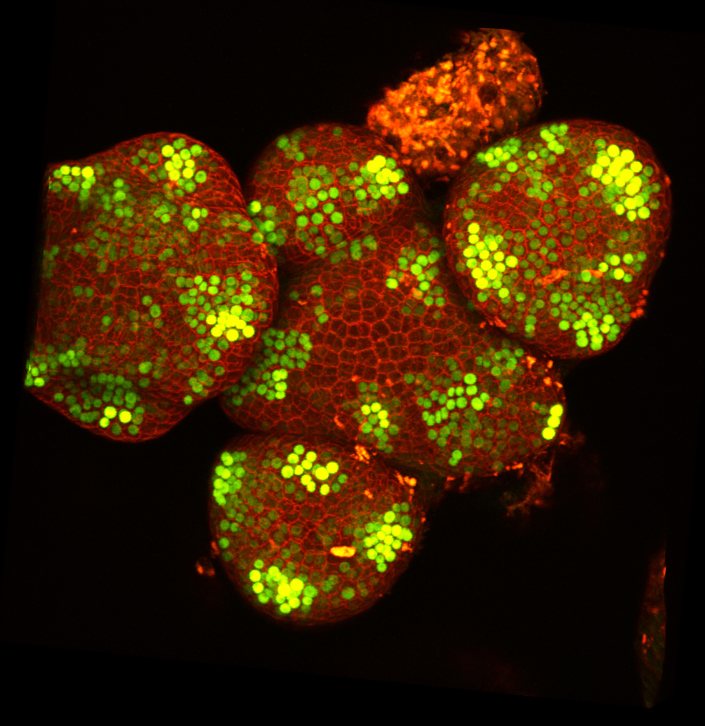
Figure 1: Inflorescence shoot apical meristem of Arabidopsis thaliana. Zones with high auxin concentration are highlighted by the fluorescent yellow signal auxin reporter from DR5::YFP. The red signal is highlighting cell walls stain, using propidium iodide.

Auxin occurs in various plant tissues, where it is transported by polar cellular transport in various directions and can explain developmental patterning phenomena such as vein formation, see e.g. Scarpella et al., (2006) or Bayer et al., (2009).

In the following, we consider the models in Jönsson et al., (2006) and Smith et al., (2006), based on polar auxin flux. Polar auxin flux results from uneven accumulation of the auxin transport regulator PIN in cell membranes. An essential component is a positive feedback between auxin flux and PIN localization, resulting in the reinforcement of polar auxin transport to dedicated routes which develop into vascular tissues. We will not enter here into these considerations, but focus on simple models of transport processes (see e.g. the discussion in Jönsson et al., (2006) and Shipman and Newell, (2005)), where a quasi-equilibrium is assumed for PIN proteins. The molecules present in some cell $i$ may be transported to any neighbouring cell $j$, but they are preferentially transported to the neighbours with the highest auxin concentrations.

Traditionally, models of patterning and morphogenesis have used reaction-diffusion theory. Turing demonstrated how, under some hypotheses, the regular patterns observed in phyllotaxis can be predicted (Turing, 1952). He showed that a combination of diffusion and a chemical reaction could give rise to regular patterns. Interesting models are described in Meinhardt, (1982); Thornley, (1975) which can, under some hypotheses, predict phyllotactic patterns. As stated previously, the auxin flux is strongly polarized, a phenomenon that cannot be described with reaction-diffusion models. The recent mathematical models given in Barbier de Reuille et al., (2006); Jönsson et al., (2006); Smith et al., (2006) are based on transport processes. Mathematically, mass transport processes are not well understood, and their study is a challenging problem. We propose here a mathematical study of related dynamical systems. We focus on their critical points and analyse their geometrical structure and stability.

Besides stable auxin peaks, the model generates intervening areas of auxin depletion, as it is observed experimentally. These auxin depleted sites reflect an indirect repulsion mechanism since auxin molecules diffusing through the tissue will be attracted to the peaks, and diverted from the depleted areas. This idea of repulsion or spacing mechanism was already considered a long time ago (Hofmeister, 1868).

The auxin flux is present everywhere in the plant, so that we choose to describe the various plant cells as a connected graph $(\Lambda,E)$. The node set $\Lambda$ represents the cells and $E$ the set of edges. Any edge $e=(i\to j)$, $i$, $j\in\Lambda$ indicates that some auxin molecule can move from cell $i$ to cell $j$. This graph is undirected, and we write $i\sim j$ to denote that cells $i$ and $j$ are nearest neighbours, so that auxin can move from cell $i$ to cell $j$, at some rate $q_{ij}$. These transition rates are not well understood at present time and one must rely on simple models. They should capture the fact that an auxin molecule present in some cell $i$ has the tendency to move to a cell $j\sim i$ when the concentration $a_{j}$ of auxin molecules present in cell $j$ is high. The simplest model accounting for this idea is given by Jönsson et al., (2006)

$$q_{ij}=\frac{a_{j}}{\kappa+\sum_{k\sim i}a_{k}},$$ (1)

for some positive constant $\kappa$, which is of Michaelis-Menten or Monod type. Let $L=|\Lambda|$ be the number of cells. In the model given in Jönsson et al., (2006) (see also Smith et al., (2006); Sahlin et al., (2009)), $a_{i}(t)$, for $i=1,\cdots,L$, denotes the concentration or the number of auxin molecules in cell $i$ at time $t$, and is assumed to evolve according to the differential equations

$$\frac{\mathrm{d}a_{i}}{\mathrm{dt}}=f_{i}({\boldsymbol{a}})=D\sum_{k\sim i}(a_{k}-a_{i})+T\sum_{k\sim i}\Big{(}a_{k}\underbrace{\frac{a_{i}}{\kappa+\sum_{j\sim k}a_{j}}}_{=q_{ki}({\boldsymbol{a}})}-a_{i}\underbrace{\frac{a_{k}}{\kappa+\sum_{j\sim i}a_{j}}}_{=q_{ik}({\boldsymbol{a}})}\Big{)},$$ (2)

for $i=1,\ldots,L$. The term $a_{i}q_{ik}$ gives the mean number of auxin molecules moving from cell $i$ to cell $k$ per unit time, and $D\sum_{k\sim i}(a_{k}-a_{i})$ is a diffusive part, usually assumed to be weak with a small diffusion coefficient $D$. The second term corresponds to the mass transport process, which is known to be the main actor of the patterning process in plants. One can add auxin production and degradation terms, but, there is no clear biological evidence about where auxin is produced, and experiments show that it is not produced in the meristem, but imported from the leaves (Reinhardt et al., 2000, 2005).

1.1 Results

Direct quantitative measurements of auxin distribution in plant tissues are very difficult due to the small size of the meristematic tissues at the time of patterning. Therefore, biologists rely on indirect markers based on auxin-regulated genes that encode fluorescent proteins. Figure 1 shows a typical output, where domains rich in auxin appear as regions of strong green fluorescence. The pattern is quite noisy; this might be due either to the indirect experiments, or to the fact that the number of auxin molecules is not too high. (2) might model the limiting behavior of this random particle system when the number of molecules tends to infinity. We introduce such a particle system in Section 2 and justify equations like (2) using law of large numbers.

We then focus on the properties of (2), like the non-negativity of the solutions (see Proposition 3.1). This dynamical system can be written in the compact form

$$\frac{\mathrm{d}{\boldsymbol{a}}}{\mathrm{dt}}=f({\boldsymbol{a}}),$$

where ${\boldsymbol{a}}(t)=(a_{i}(t))_{1\leq i\leq L}$ is the vector of auxin concentrations. The related critical points are the vectors ${\boldsymbol{a}}^{*}$ satisfying $f({\boldsymbol{a}}^{*})=0$. They are the candidates for describing the equilibrium auxin concentrations. For example, $a_{i}=0$ means that there is (almost) no auxin molecules in cell $i$, while a subset of cells $J$ such that $a_{j}>0$ for $j\in J$ indicates a hot spot which might correspond to an auxin peak.

The critical points play a fundamental role in the dynamic, and one can suspect that any solution ${\boldsymbol{a}}(t)$ of (2) will approach such critical points as $t$ is large. Of course, this is wrong for general dynamical systems, but here, the model is supposed to catch pieces of biological reality, and the robustness of the regular geometries observed in plants suggests that this might well be the case. Some of these critical points are repulsive or unstable, that is, the orbits or the solutions of (2) will avoid them. In the contrary, some of them will be attractive. Given a critical point ${\boldsymbol{a}}^{*}$, a mathematical way of checking the stability or the unstability of ${\boldsymbol{a}}^{*}$ is to compute the Jacobian ${\rm d}f({\boldsymbol{a}}^{*})$, by retaining only its spectrum, that is the set of all eigenvalues of ${\rm d}f({\boldsymbol{a}}^{*})$. For example, ${\boldsymbol{a}}^{*}$ is unstable when there is an eigenvalue having a positive real part.

Definition 1.1

We say that a critical point ${\boldsymbol{a}}$ is stable when all the eigenvalues of the Jacobian evaluated at ${\boldsymbol{a}}$ have non-positive real parts.

Section 5 is concerned with the characterization of the set of critical points, mainly focusing on pure transport processes.

For $D=0$, we first consider critical points ${\boldsymbol{a}}>0$, meaning that $a_{i}>0$ for all $i$. Corollary 5.3 shows that such elements are precisely the positive solutions of the linear equation

$$\Gamma{\boldsymbol{a}}=c\ {\bf 1},\ c\text{ constant},$$ (3)

where $\Gamma$ is the adjacency matrix of the graph $G$, with entries $\Gamma_{ij}\in\{0,1\}$ such that $\Gamma_{ij}=1$ if and only if cells $i$ and $j$ are nearest neighbours, and ${\bf 1}$ is the vector having all components equal to 1.

Next, we focus on critical points such that $a_{i}=0$ for $i$ belonging to some subset $I\subset\Lambda=\{1,\cdots,L\}$. They correspond to auxin depleted cells. The graph decomposes into a product of sub-graphs $\gamma$, which are the connected components of the sub-graph of $G$ induced by the node set $J=\Lambda\setminus I$. We thus look for ${\boldsymbol{a}}$ having positive components $a_{j}>0$ for $j\in J$, which should correspond in some sense to auxin peaks. We obtain the distribution of auxin in such components, denoted by ${\boldsymbol{a}}|_{\gamma}$, by solving the linear systems ${\Gamma_{\gamma}{\boldsymbol{a}}|_{\gamma}=c_{\gamma}{\bf 1}|_{\gamma}}$. A typical example of such configurations is given in Figure 3, where the elements of $I$ are black and the various components $\gamma$ red.

We then turn to the asymptotic behavior of the solutions of system (2), and establish in Proposition 6.3 that every solution converges toward the set of critical points. Our technique is based on Lyapunov functions, that is, we look for a function $H({\boldsymbol{a}})$ which should be decreasing along the orbits of (2), like energy in physics. We proved that, for pure transport processes with $D=0$, the function

$$H({\boldsymbol{a}})=-\kappa\langle{\bf 1},{\boldsymbol{a}}\rangle-\frac{1}{2}\langle{\boldsymbol{a}},\Gamma{\boldsymbol{a}}\rangle,$$

where $\langle\cdot,\cdot\rangle$ denotes the scalar product, satisfies

$$\frac{{\rm d}H({\boldsymbol{a}}(t))}{{\rm d}t}\leq 0$$

for any solution of (2). Newell et al., (2008) also considered the differential system (2) by taking a spatial continuous limit, and showed that the limiting equation is a p.d.e. similar to the von Karman equations from nonlinear elasticity theory:

$$\frac{\partial w}{\partial t}=\triangle^{2}w+P\triangle w+\mathrm{const}\cdot w+\text{ nonlinear terms}.$$

The von Karman equations are of gradient type (see e.g. Shipman and Newell, (2005)), where the potential is given by the elastic energy. These energy functionals were then used in Newell et al., (2008) and Newell and Shipman, (2005) to provide a very interesting mechanical explanation of the appearance of Fibonacci numbers in plant patterns based on buckling. However, the limiting equations associated with the auxin flux are not of gradient type, see the discussion in Newell et al., (2008). For the basic dynamical system (2), our result shows that the system is minimizing the energy $H$, without being of gradient type.

Section 7 considers stability, and Proposition 7.1 shows that the Jacobian ${\rm d}f({\boldsymbol{a}})=(\partial f_{i}/\partial a_{j})$ evaluated at ${\boldsymbol{a}}$ is given by

$${\rm d}f({\boldsymbol{a}})=\frac{1}{N^{2}}d({\boldsymbol{a}})\Gamma\Big{(}c\ {\rm id}-d({\boldsymbol{a}})\Gamma\Big{)},$$

where $d({\boldsymbol{a}})$ is the diagonal matrix of diagonal given by ${\boldsymbol{a}}$. This permits to check the stability of the critical points for various graphs. We present various results on graphs of interest for plant patterning questions, like the circle or the two-dimensional grid. As stated previously, the positive solutions ${\boldsymbol{a}}|_{\gamma}$ to the linear system $\Gamma_{\gamma}{\boldsymbol{a}}|_{\gamma}=c_{\gamma}{\bf 1}|_{\gamma}$ provide restrictions of the critical points to the connected components $\gamma$. We give a particularly simple condition on the sub-graph $\gamma$ of $G$ induced by the set $J=\Lambda\setminus I$ ensuring the non-stability of ${\boldsymbol{a}}|_{\gamma}$. Let ${\cal N}_{i}$, $i\in\Lambda$ be the neighbourhood of $i$, that is the set of nodes $j$ such that $j\neq i$ and $j\sim i$. The configuration ${\boldsymbol{a}}|_{\gamma}$ is unstable when the sub-graph $\gamma$ contains a path of length 4, of the form

$$i_{0}\to i_{1}\to i_{2}\to i_{3},$$

such that

$$i_{1}\in{\cal N}_{i_{0}},\ i_{2}\not\in{\cal N}_{i_{0}}\text{ and }i_{3}\not\in{\cal N}_{i_{0}}.$$

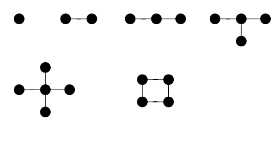
Figure 2: Example of components $\gamma$ of the two-dimensional grid that can potentially yield stable configurations, see Corollary 7.3.

For example, if $G$ is a two-dimensional grid, any stable configuration is composed of patches of the basic building blocks given in Figure 2; These patterns are however not geometrically regular in general, see Figure 3. The more involved model of Smith et al., (2006), which uses PIN proteins in a direct way (here we assume a quasi-equilibrium, see Jönsson et al., (2006)), produces more regular patterns in simulations. In this setting, the transition rates are forced to follow exponential distributions. Hence, a strong selection based on rates of the form $\exp(ba_{i})$, $b>0$ instead of the linear function $a_{i}$ seems to regularize the critical points. Of course, it might be interesting to justify such a choice biologically. We also argue in what follows that the critical configurations produced by the auxin flux might be more regular when coupled to periodic potentials.

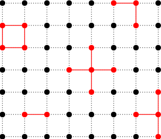
Figure 3: A potentially stable configuration when the graph $G$ is a rectangular grid, for the pure transport process. The black circles correspond to the values $a_{i}=0$, $i\in I$ (the set auxin depleted cells), while the red circles are such that $a_{i}>0$, corresponding to auxin peaks. One can construct the set of all stable configurations by playing with the building block given by the square, the star, and the various parts of the star. This shows that dynamical system (2) does not necessarily produce regular patterns. We can however give examples where such configurations are unstable, see Section 7.3

It might well be that the auxin flux self-organize in regular patterns when coupled to mechanical forces, for example, as already stated in the Introduction, see Newell et al., (2008). In the same spirit, we introduce a simple model coupling the auxin flux to a potential $\phi$, which might model deformations, curvature or effects related to the meristem elasticity. We provide an example of the form

$$\frac{{\rm d}a_{i}(t)}{{\rm d}t}=f_{i}({\boldsymbol{a}})+\sum_{j\sim i}(a_{j}\phi_{i}-a_{i}\phi_{j}),$$ (4)

$i=1,\ldots,L$. If the potential itself has some regularities, as it is the case in specific model given in Newell et al., (2008), the auxin flux will exhibit much more regular patterns, see e.g. Figure 4.

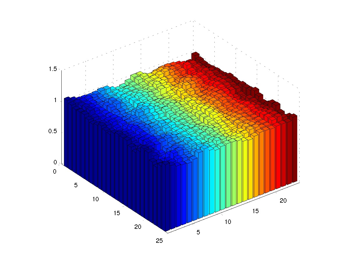
(a) ${\boldsymbol{a}}(t)$ for $t\approx 0$

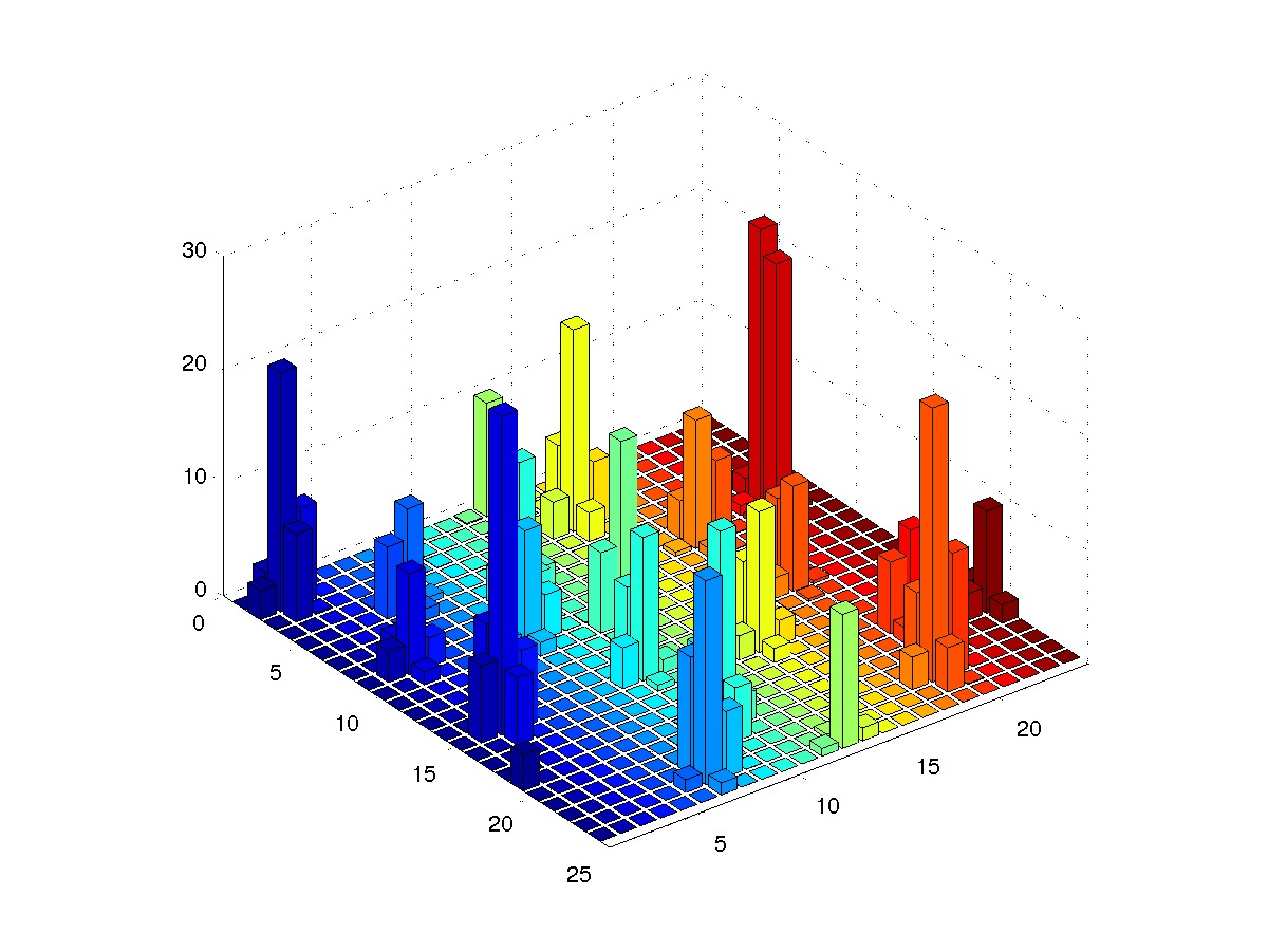
(b) ${\boldsymbol{a}}(t)$ for large $t$.

Figure 4: Simulation of the orbits of the differential equation (4) with $T=1,D=0$ and a potential $\phi(x,y)=\sin(4\pi x/A)\sin(4\pi y/B)$ on a torus, where $x=1,\cdots,A$ and $y=1,\cdots,B$. The initial state is flat. (b) shows the state ${\boldsymbol{a}}(t)$ for large $t$: one sees regularly spaced auxin peaks, which are isolated in a background of auxin depleted cells. The potential and transport terms drift thus the process toward more regular patterns, while the transport process creates domains of auxin depletion.

Finally, the model provides an interesting conclusion: for most graphs, stable configuration are composed of building blocks isolated in a sea of auxin depleted cells. This might be the basis for repulsion between primordia: auxin molecules will not have the tendency to move toward them, leading to indirect repulsion. The idea of such repulsive force appeared a long time ago in the work of Hofmeister, (1868). Many authors have used this hypothesis to develop very interesting mathematical models, all leading to phyllotactic patterns observed in nature, like Fibonacci numbers, the Golden Angle or helical lattices, see Adler, (1974); Atela et al., (2002); Douady and Couder, (1996); Kunz, (1995); Levitov, (1991).

2 A stochastic model of auxin transport

We consider a stochastic process related to differential equation (2), describing the random numbers of auxin molecules $\eta_{t}(i)\in\mathbb{N}$ present in cell $i$ at time $t$, $i=1,\cdots,L$. The state space of this stochastic process is denoted by $\Omega_{L}=\mathbb{N}^{\Lambda}$, where $\Lambda$ is the set of $L$ cells (the nodes of the graph). Looking at equation (2), we define transitions by supposing that any auxin molecule present in cell $i$ at time $t$ can be transported to a neighboring cell $j$ at rate $\bar{q}_{ij}(\eta)$ of the form

$$\bar{q}_{ij}(\eta)=\frac{\eta(j)}{\bar{\kappa}+\sum_{k\sim i}\eta(k)},$$ (5)

when $\eta(i)\geq 1$. This defines a Markov process with state space $\Omega_{L}$, describing the stochastic moves of the various auxin molecules. Let $M$ denote the total number of molecules. It turns out that the ordinary differential equation (2) describes the large $M$ limit of the stochastic process (weak noise limit). This random particle system is then described as a gaussian process $X_{M}(t)\approx\eta_{t}/M$ in $\mathbb{R}^{L}$ drifted by the solution ${\boldsymbol{a}}(t)$ of (2) for some covariance function. This approximation will be mathematically rigourous if the constants $\kappa$ and $\bar{\kappa}$ are related in such a way that $\bar{\kappa}=M\kappa$, and the limiting behavior of the rescaled number of auxin molecules is such that $\eta_{t}(i)/M\approx a_{i}(t)$, where ${\boldsymbol{a}}(t)$ solves (2), with $\sum_{i\in\Lambda}a_{i}(t)\equiv 1$.

Such stochastic particle systems are known as density dependent population processes, and the above limit has been treated in detail in Ethier and Kurtz, (1986), and corresponds to a law of large numbers. Notice that different kinds of limits can also be considered. Stochastic mass transport processes of this type have also appeared in physics, and are known as generalized zero range processes, see e.g. Evans et al., (2006); Luck and Godrèche, (2007); Grosskinsky et al., (2011); Kipnis and Landim, (1999). In this setting, hydrodynamical limits are considered, when both $M$ and $L$ tend simultaneously to $\infty$ in such a way that $M=\rho L$, for a fixed density. Simulations show the appearance of condensates when $\rho$ is larger than a critical threshold $\rho_{c}$, which might represent auxin peaks in some way. Mathematically, the theory of condensation is not developed at present time for these general processes, so that we here focus on the weak noise limit.

The gaussian approximation of $\eta_{t}/M$ is defined as follows: for $i=1,\cdots,L$, consider the unit vectors $e_{i}$ with $e_{i}(j)=0$ when $j\neq i$ and $e_{i}(i)=1$. Let ${\rm d}f$ be the Jacobian ${\rm d}f=(\partial f_{i}/\partial a_{j}))_{i,j=1,\cdots,L}$.

For simplicity, we illustrate the transition rates for cells arranged along a circle: the rate functions are given by functions $\beta_{l}({\boldsymbol{a}})$, $l\in\mathbb{Z}^{l}$, satisfying

$$\beta_{e_{i+1}-e_{i}}({\boldsymbol{a}}) =(Da_{i}+T\frac{a_{i+1}a_{i}}{\kappa+a_{i-1}+a_{i+1}})\ ; \mathrm{for}\;i=1,\ldots,L,$$

$$\beta_{e_{i-1}-e_{i}}({\boldsymbol{a}}) =(Da_{i}+T\frac{a_{i-1}a_{i}}{\kappa+a_{i-1}+a_{i+1}})\ ; \mathrm{for}\;i=1,\ldots,L,$$

$$\beta_{l}({\boldsymbol{a}}) =0 \mathrm{for}\ ;l\neq e_{i-1}-e_{i},e_{i+1}-e_{i}.$$

For example $e_{i+1}-e_{i}$ means that an auxin molecule of cell $i$ has been transported in cell $i+1$. For arbitrary graphs, the definitions of the rates $\beta_{l}$ are similar.

With these notations, we can define the matrix $G$

$$G({\boldsymbol{a}})=\sum_{l\in\mathbb{Z}^{L}}\beta_{l}({\boldsymbol{a}})ll^{*},$$

which will be an essential element of the covariance matrix associated with the gaussian approximation. Consider the following matrix valued differential equation

$$\frac{\partial\phi(t,s)}{\partial t}={\rm d}f({\boldsymbol{a}}(t))\phi(t,s),\ \ \phi(s,s)={\rm id}.$$

Then, as $M$ is large, one gets that (see e.g. (Ethier and Kurtz, 1986))

$$\frac{\eta_{t}}{M}={\boldsymbol{a}}(t)+\frac{1}{\sqrt{M}}V_{t},$$

where $V_{t}$ is a gaussian process of mean $\phi(t,0)V(0)$ and of covariance function

$${\rm Cov}(V(t),V(r))=\int_{0}^{\min\{t,r\}}\phi(t,s)G({\boldsymbol{a}}(s))\phi(r,s)^{*}{\rm d}s.$$

3 Basic properties of the auxin flux

Proposition 3.1

Every solution ${\boldsymbol{a}}$ of (2) starting in $\mathbb{R}^{L}_{\geq 0}$ remains non-negative, and is conservative, that is,

$$\forall t\in\mathbb{R}_{\geq 0},\;\sum_{i}^{L}a_{i}(t)=\sum_{i}^{L}a_{i}(0)=\rho L.$$

Moreover, the system (2) admits a unique solution defined over $[0,+\infty)$. When $a_{i}(0)>0$, then $a_{i}(t)>0$, $\forall t>0$. For pure transport processes with $D=0$, $a_{i}(0)=0\Rightarrow a_{i}(t)\equiv 0,\ \forall t>0$.

The proof of proposition 3.1 is given in Section 8.

Let us rewrite the system (2), for $1\leq i\leq L$

$$\dot{a}_{i}=D\sum_{k\sim i}a_{k}+T\sum_{k\sim i}(\frac{a_{k}}{\kappa+\sum_{j\sim k}a_{j}}-\frac{a_{k}}{\kappa+\sum_{j\sim i}a_{j}}-\frac{D}{T})a_{i},$$ (6)

with the initial condition ${\boldsymbol{a}}(0)\in\mathbb{R}_{+}^{L}$.

Proposition 3.2

If the graph is connected and $D>0$, the only critical point of (6) in $\mathbb{R}_{+}^{L}$ admitting zero components is the origin.

Proof.

Let $a_{i}=0$ where $a_{i}$ is the $i$-th component of a critical point $a\in\mathbb{R}_{+}^{L}$ of (6). Clearly (6) entails $\sum_{k\sim i}a_{k}=0$ and the non-negativity of each term, $a_{k}=0$ for all $k\sim i$. Since the graph is connected we deduce that $a_{k}=0$ for all $1\leq k\leq L$. ∎

Proposition 3.3

Let us assume that the graph is connected and $D>0$. If $\sum_{k=1}^{L}a_{k}(0)>0$, then for all $i\in\{1,...,L\}$, we have $\underline{\lim}_{t\rightarrow+\infty}a_{i}(t)>0.$

To prove the previous proposition, we will use the following Proposition, see Gabriel et al., (1989).

Proposition 3.4

Let $f:\mathbb{R}_{+}\rightarrow\mathbb{R}$ be twice differentiable and bounded together with $\ddot{f}$. If, as $n\rightarrow+\infty$, $t_{n}\uparrow+\infty$ and $f(t_{n})\rightarrow\underline{\lim}_{t\rightarrow+\infty}f(t)$ (or $f(t_{n})\rightarrow\overline{\lim}_{t\rightarrow+\infty}f(t)$), then $\dot{f}(t_{n})\rightarrow 0$.

Remark 3.5

1. The boundedness of $f$ and $\ddot{f}$ implies the one of $\dot{f}$.

2. The assumptions in the preceding proposition can be weakened without changing essentially the proof: "$f:\mathbb{R}_{+}\rightarrow\mathbb{R}$ be twice differentiable and bounded together with $\ddot{f}$ " can be replaced by "$f:\mathbb{R}_{+}\rightarrow\mathbb{R}$ is bounded and differentiable and $\dot{f}$ is uniformly continuous".

Proof.

If $a_{k}(0)=0$ for all $1\leq k\leq L$, then the unique solution is identically zero. Otherwise $\sum_{k=1}^{L}a_{k}(0)>0$. Let us suppose that for some $i\in\{1,...,L\}$,

$$\underline{\lim}_{t\rightarrow+\infty}a_{i}(t)=0.$$

Let us introduce the notation $\underline{a}_{i}=\underline{\lim}_{t\rightarrow+\infty}a_{i}(t)$. Since $a_{i}(t)$ is bounded together with its second derivative, the preceding proposition applies and for any sequence $t_{n}\uparrow+\infty$ such that $a_{i}(t_{n})\rightarrow\underline{a}_{i}$, we have $\dot{a}_{i}(t_{n})\rightarrow 0$ as $n\rightarrow+\infty$. Every $a_{k}(t_{n})$ being bounded in the right-hand member of the equation for $\dot{a}_{i}(t_{n})$, we conclude that $\lim_{n\rightarrow+\infty}D\sum_{k\sim i}a_{k}(t_{n})=0$. The non-negativity of each $a_{k}(t_{n})$ entails $\lim_{n\rightarrow+\infty}a_{k}(t_{n})=0=\underline{a}_{k}$ for every ${k\sim i}$. According to the above proposition, $\lim_{n\rightarrow+\infty}\dot{a}_{k}(t_{n})=0$ for every ${k\sim i}$ and since the graph is connected, repeating the same argument provides $\lim_{n\rightarrow+\infty}\dot{a}_{j}(t_{n})=0$ for every $j\in\{1,...,L\}$. Thus $0=\lim_{n\rightarrow+\infty}\sum_{1\leq j\leq L}a_{j}(t_{n})=\sum_{k=1}^{L}a_{k}(0)>0$, a contradiction.

As a consequence, for $D>0$, it is impossible to have $\lim_{t\rightarrow+\infty}a_{i}(t)=0$, and thus none of the compartments can become empty asymptotically. ∎

4 Tools from Markov Chain theory

We will use notions from Markov chain theory, and hence consider generators $Q:\ \Lambda\ {\rm x}\ \Lambda\longrightarrow\mathbb{R}$, $Q=\{q_{ij},\ i,\ j\in\Lambda\}$, such that

$$q_{ij}\geq 0,\ \text{ for }i\neq j\text{ and }q_{ii}=-\sum_{j\neq i}q_{ij}.$$

For example, the auxin flux described by (2) contains implicitly a generator $Q(D,T,{\boldsymbol{a}})$ given by

$$\begin{cases}q_{ij}(D,T,{\boldsymbol{a}})=D+Tq_{ij}({\boldsymbol{a}}),&i\sim j,\\ q_{ij}(D,T,{\boldsymbol{a}})=0,&i\nsim j,i\neq j.\\ q_{ii}(D,T,{\boldsymbol{a}})=-\sum_{j\neq i}q_{ij}(D,T,{\boldsymbol{a}}),\end{cases}$$ (7)

where we set

$$q_{ij}({\boldsymbol{a}})=\frac{a_{j}}{\kappa+\sum_{k\sim i}a_{k}}.$$

$Q$ is irreducible when for any pair of nodes $(i,j)$, there is a path $i_{0}=i\to i_{1}\to i_{2}\to\cdots\to i_{k}=j$ such that $q_{i_{n}i_{n+1}}>0$, $n=0,\cdots,k-1$. When $Q$ is irreducible, one can prove that there is a unique invariant probability measure $\pi$ satisfying $\pi^{*}Q=0$.

An irreducible transition kernel $Q$ of invariant probability measure $\pi$ is said to be reversible when

$$\pi_{i}q_{ij}\equiv\pi_{j}q_{ji},\ \forall i\neq j.$$

5 Characterization of the critical points

We can write (2) in the more compact form

$$\frac{\mathrm{d}a_{i}}{\mathrm{dt}}=f_{i}({\boldsymbol{a}})=\sum_{j\sim i}(a_{j}q_{ji}(D,T,{\boldsymbol{a}})-a_{i}q_{ij}(D,T,{\boldsymbol{a}})),\ \ \frac{\mathrm{d}{\boldsymbol{a}}}{\mathrm{dt}}=f({\boldsymbol{a}})={\boldsymbol{a}}^{\ast}Q(D,T,{\boldsymbol{a}}).$$

Our first aim is to look for the critical points of the above dynamical system, that is, to find the element ${\boldsymbol{a}}\in\mathbb{R}^{L}$ solving the equations $f({\boldsymbol{a}})=0$, which can be rewritten as ${\boldsymbol{a}}^{\ast}Q(D,T,{\boldsymbol{a}})=0$. Hence, any solution to $f({\boldsymbol{a}})=0$ is an invariant measure associated with the transition function $Q(D,T,{\boldsymbol{a}})$. We will use the following facts:

• When $D>0$, the generator $Q(D,T,{\boldsymbol{a}})$ is irreducible.

• For pure transport processes where $D=0$ and $T>0$, $Q(0,T,{\boldsymbol{a}})$ is irreducible if and only if $a_{i}>0$ $\forall i$.

In the irreducible case, let $\pi({\boldsymbol{a}})$ denote the associated positive invariant probability measure. We thus look for ${\boldsymbol{a}}>0$ such that

$$\frac{{\boldsymbol{a}}}{\sum_{i\in\Lambda}a_{i}}=\pi({\boldsymbol{a}}).$$ (8)

5.1 The irreducible case

Pure transport processes

If $Q(0,T,{\boldsymbol{a}})$ is reversible, the equation $f({\boldsymbol{a}})=0$ is equivalent to the set of equations

$$a_{i}q_{ij}(0,T,{\boldsymbol{a}})\equiv a_{j}q_{ji}(0,T,{\boldsymbol{a}}),\ \ i\neq j.$$ (9)

In what follows, we will use the functions

$$N_{k}=N_{k}({\boldsymbol{a}})=\kappa+\sum_{j\sim k}a_{j}.$$ (10)

Lemma 5.1

Let $G$ be a connected graph. Assume that $D=0$ and $T>0$. Then $Q(0,T,{\boldsymbol{a}})$ is reversible $\forall{\boldsymbol{a}}>0$, of invariant probability measure given by

$$\pi({\boldsymbol{a}})=\Big{(}\frac{a_{i}N_{i}}{Z({\boldsymbol{a}})}\Big{)}_{i\in\Lambda},$$ (11)

where

$$Z({\boldsymbol{a}})=\sum_{i\in\Lambda}a_{i}N_{i}=\kappa\sum_{i\in\Lambda}a_{i}+\sum_{i\in\Lambda}\sum_{j\sim i}a_{i}a_{j}.$$

In this case, ${\boldsymbol{a}}>0$ is a critical point with $f({\boldsymbol{a}})=0$ if and only if $N_{i}({\boldsymbol{a}})$ does not depend on $i$, with

$$N_{i}({\boldsymbol{a}})\equiv\frac{Z({\boldsymbol{a}})}{\sum_{i\in\Lambda}a_{i}}=\kappa+\frac{\sum_{i\in\Lambda}\sum_{j\sim i}a_{i}a_{j}}{\sum_{i\in\Lambda}a_{i}}.$$ (12)

Remark 5.2

The transition rates $q_{ij}({\boldsymbol{a}})$ are similar to the rates associated with a family of Markov chains used in the study of vertex-reinforced random walks, see Benaïm, (1997); Benaïm and Tarrès, (2008) and Pemantle, (1992), and Lemma 5.1 is an adaptation of these results. Interestingly, such vertex-reinforced random walks are approximated by deterministic dynamical systems called replicator dynamics, of the form

$$\frac{{\rm d}a_{i}}{{\rm d}t}=a_{i}(N_{i}^{\prime}({\boldsymbol{a}})-H^{\prime}({\boldsymbol{a}})),$$

where $N_{i}^{\prime}({\boldsymbol{a}})=N_{i}({\boldsymbol{a}})-\kappa$ and $H^{\prime}({\boldsymbol{a}})=\sum_{i\in\Lambda}a_{i}N_{i}^{\prime}$. In this setting, the function $H^{\prime}$ plays the role of a Lyapunov function. We will also find a similar Lyapunov function, see Section 6.

Proof.

Assume, without loss of generality, that $T=1$. First notice that

$$\sum_{j\sim i}\pi({\boldsymbol{a}})_{j}q_{ji}(0,T,{\boldsymbol{a}}) = \sum_{j\sim i}\frac{a_{j}N_{j}}{Z({\boldsymbol{a}})}\frac{a_{i}}{N_{j}}$$

$$= \frac{1}{Z({\boldsymbol{a}})}\sum_{j\sim i}a_{i}a_{j}=\frac{a_{i}}{Z({\boldsymbol{a}})}\sum_{j\sim i}a_{j}=\frac{a_{i}(N_{i}-\kappa)}{Z({\boldsymbol{a}})}.$$

The identity

$$\pi({\boldsymbol{a}})_{i}q_{ii}(0,T,{\boldsymbol{a}})=-\frac{a_{i}N_{i}}{Z({\boldsymbol{a}})}\sum_{j\sim i}\frac{a_{j}}{N_{i}}=-\frac{a_{i}(N_{i}-\kappa)}{Z({\boldsymbol{a}})},$$

shows that

$$\sum_{j\sim i}\pi({\boldsymbol{a}})_{j}q_{ji}(0,T,{\boldsymbol{a}})+\pi({\boldsymbol{a}})_{i}q_{ii}(0,T,{\boldsymbol{a}})=0,$$

so that $\pi({\boldsymbol{a}})$ is a invariant probability measure for $Q(0,T,{\bf a})$. $\bf{a}>0$ is a critical point with $f({\boldsymbol{a}})=0$ if and only if $\frac{{\boldsymbol{a}}}{\sum_{i\in\Lambda}a_{i}}$ is an invariant measure for $Q(0,T,{\bf a})$. Because of the unicity of the invariant measure, we obtain

$$N_{i}({\boldsymbol{a}})\equiv\frac{Z({\boldsymbol{a}})}{\sum_{i\in\Lambda}a_{i}}.$$

∎

Let $\Gamma$ be the adjacency matrix of the graph $G=(\Lambda,E)$, that is, the matrix with entries given by $\Gamma_{ij}=1$, when $i\neq j$ and $i\sim j$, and $\Gamma_{ij}=0$ otherwise. We summarize the above results in the following

Corollary 5.3 (Pure Transport Processes)

Assume that $D=0$ and $T>0$ (no diffusion), and consider only positive ${\boldsymbol{a}}>0$. Then,

$$f({\boldsymbol{a}})=0\hbox{ if and only if }\Gamma{\boldsymbol{a}}=c({\boldsymbol{a}}){\rm\bf 1},\ {\rm\bf 1}=(1,\cdots,1)^{*},$$ (13)

where

$$c({\boldsymbol{a}})=\frac{\sum_{i\in\Lambda}\sum_{j\sim i}a_{i}a_{j}}{\sum_{i\in\Lambda}a_{i}}=\frac{\langle{\boldsymbol{a}},\Gamma{\boldsymbol{a}}\rangle}{\langle{\boldsymbol{a}},{\bf 1}\rangle}.$$ (14)

Remark 5.4

Let $c$ be a constant, and let ${\boldsymbol{a}}$ (if it exists) be such that $\Gamma{\boldsymbol{a}}=c{\bf 1}$ and ${\bf a}\geq 0$. Then ${\bf a}$ is a critical point and $c$ is given by (14).

Example 5.5 (The one-dimensional cycle)

Assume that the $L$ cells are arranged on a cycle. The pure transport process ($D=0$) is reversible, so that the critical points ${\boldsymbol{a}}>0$ of dynamical system (2) are solutions of linear system (13). We illustrate some results given in Section 7.4. When $L>4$ is a multiple of 4, the set of critical points ${\boldsymbol{a}}\in\mathbb{R}^{L}$ forms a two dimensional sub-manifold $M_{c}$ of $\mathbb{R}^{L}$ given by, when $\rho=1/L$,

$$M_{c}=\{(a_{1},a_{2},-a_{1}+2\rho,-a_{2}+2\rho,a_{1},a_{2},-a_{1}+2\rho,-a_{2}+2\rho,\cdots);\ a_{k}\in(0,2\rho),\ k=1,2\}.$$

When $L>4$ is not a multiple of 4, $M_{c}$ is reduced to the uniform configuration $M_{c}=\{(\rho,\rho,\cdots,\rho)\}$. We will see that the uniform configuration is always unstable, and that the other critical points are unstable when ${\boldsymbol{a}}>0$. However, the boundary points are all stable.

General transport processes

Lemma 5.6

Assume that $G$ is connected, and that both $D$ and $T$ are positive. For ${\boldsymbol{a}}>0$, $f({\boldsymbol{a}})=0$ if and only if there exists a constant $c$ such that ${\boldsymbol{a}}$ solves the following system of quadratic equations:

$$(a_{i}-\frac{D}{T})N_{i}({\boldsymbol{a}})+a_{i}=c\ a_{i}N_{i}({\boldsymbol{a}}),\ i=1,\cdots,\ \Lambda.$$ (15)

Proof.

Let $\mu_{i}=(a_{i}-D/T)N_{i}$, $i=1,\cdots,\Lambda$. Then ${\boldsymbol{\mu}}=(\mu_{i})_{1\leq i\leq\Lambda}$ behave

$$(\mu Q(0,T,{\boldsymbol{a}}))_{i} = \sum_{j\sim i}\mu_{j}q_{ji}({\boldsymbol{a}})+\mu_{i}q_{ii}({\boldsymbol{a}})$$

$$= T\sum_{j\sim i}(a_{j}-\frac{D}{T})N_{j}\frac{a_{i}}{N_{j}}-T(a_{i}-\frac{D}{T})N_{i}\sum_{j\sim i}\frac{a_{j}}{N_{i}}$$

$$= T\sum_{j\sim i}(a_{j}-\frac{D}{T})a_{i}-T(a_{i}-\frac{D}{T})\sum_{j\sim i}a_{j}$$

$$= T\frac{D}{T}\sum_{j\sim i}(a_{j}-a_{i}),$$

which gives the diffusion term contained in $f$. Hence, one can rewrite the equation $f({\boldsymbol{a}})=0$ as

$$({\boldsymbol{\mu}}+{\boldsymbol{a}})Q(0,T,{\boldsymbol{a}})=0.$$

By assumption, ${\boldsymbol{a}}>0$ so that $Q(0,T,{\boldsymbol{a}})$ is irreducible as a Markov generator, and hence has only one invariant probability measure. The linear space composed of invariant measures is one-dimensional, so that the measure ${\boldsymbol{\mu}}+{\boldsymbol{a}}$ is proportional to $\pi({\boldsymbol{a}})$. The result is a consequence of expression for $\pi({\boldsymbol{a}})$ given in (11). ∎

The next paragraph generalizes the diffusive part to model the effect of potentials on the auxin flux.

Inclusion of potentials

As stated in the Introduction, experiments have shown that both mechanical and biochemical processes play a role in plant patterning. We here adapt some ideas of Newell et al., (2008) and Newell and Shipman, (2005) to our discrete setting. The former considered the discrete model (2) by taking a continuous limit, resulting in a p.d.e. describing the time evolution of auxin concentrations, which is coupled to the von Karman equations from elasticity theory. These equations describe the deformations of an elastic shell or plate subject to various loading conditions. Usually, the in-plane stress is described using Airy functions which are potential for the stress field. Here, we will simply suppose that this potential is given by some function $(\phi_{i})_{1\leq i\leq L}$. We also suppose that the auxin flux is directed in part by these potentials and assume a model of the form

$$\frac{{\rm d}a_{i}(t)}{{\rm d}t}=f_{i}({\boldsymbol{a}})+\sum_{j\sim i}(a_{j}\phi_{i}-a_{i}\phi_{j}),$$ (16)

$i=1,\ldots,L$. We will see in the sequel that the critical points associated to (2) exhibit regular geometrical patterns locally, but not necessarily globally. The potential might be defined in such a way to reproduce the patterns obtained when considering mechanical buckling, and the model defined by (16) might then lead to more regularly spaced auxin peaks, see Figure 4.

Lemma 5.7

Assume a model of the form (16), with $D>0$ and $T>0$. Let ${\boldsymbol{a}}>0$. Then $f_{i}({\boldsymbol{a}})+\sum_{j\sim i}(a_{j}\phi_{i}-a_{i}\phi_{j})=0$ if and only if there exists a constant $c\in\mathbb{R}$ such that

$$(a_{i}-\frac{D}{T}-\frac{1}{T}\phi_{i})N_{i}({\boldsymbol{a}})+a_{i}=c\ a_{i}N_{i}({\boldsymbol{a}}),\ i=1,\cdots,\Lambda.$$

The proof of Lemma 5.7 is identical to the proof of Lemma 5.6.

5.2 The reducible case

We can adapt the previous notions to the case $D=0$ and reducible transition kernel $Q(0,T,{\boldsymbol{a}})$, that is when some $a_{i}$ vanish. In this case, there is a pair of nodes $i$ and $j$ such that

$$\prod_{k=1}^{m}q_{i_{k-1}i_{k}}({\boldsymbol{a}})=0,$$

for all paths $\gamma:\ i_{0}=i\to i_{1}\to\cdots\to i_{m}=j$ taking $i$ to $j$ in the graph $G=(\Lambda,E)$.

Example 5.5 shows that the critical points associated with (2) on a circle form a manifold when $L$ is a multiple of 4. We also assert that the boundary points obtained from $M_{c}$ by setting $a_{1}=0$ are stable. We will thus consider subsets $I\subset\{1,\cdots,L\}$ corresponding to the sites $i$ where $a_{i}=0$. We will denote by ${\boldsymbol{a}}|_{I}$ the restriction of any ${\boldsymbol{a}}$ to $I$. The same notations apply for generators and adjacency matrices, where one conserves only the transitions rates $q_{ij}({\boldsymbol{a}})$ such that $i$, $j\in\Lambda\setminus I$. According to Lemma 5.1, these sub-transition kernels are reversible for ${\boldsymbol{a}}$ such that $a|_{\Lambda\setminus I}>0$. If one removes the nodes $i\in I$, the graphs decomposes as a product of connected components $\gamma$, which form the sub-graph of $G$ induced by the nodes of $J=\Lambda\setminus I$. The special form of the vector field associated with (2) ensures however that the set of critical values such that ${\boldsymbol{a}}|_{I}=0$, $I\subset\{1,\cdots,L\}$, can be obtained by considering a family of transitions functions $Q_{\gamma}(0,T,{\boldsymbol{a}}|_{\gamma})$. For each component $\gamma$, Corollary 5.3 shows that the related critical points are obtained by solving linear systems of the form

$$\Gamma_{\gamma}{\boldsymbol{a}}|_{\gamma}=c_{\gamma}{\rm\bf 1}|_{\gamma},$$ (17)

where $\Gamma_{\gamma}$ is the adjacency matrix of the sub-graph $\gamma$, and the $c_{\gamma}$ are normalization constants chosen in such a way that $\sum_{i}a_{i}=\rho L$. The set of critical points is then obtained by taking the direct product of the sets of critical values associated with the sub-graphs $\gamma$.

6 Asymptotic properties of the auxin flux for pure transport processes

We consider the convergence of the dynamical system (2) when $D=0$ using the method of Lyapunov functions. Suppose without loss of generality that $T=1$. We look for a function $H({\boldsymbol{a}})$ such that

$$\frac{{\rm d}H({\boldsymbol{a}}(t))}{{\rm d}t}=\langle\nabla H({\boldsymbol{a}}(t)),\frac{{\rm d}{\boldsymbol{a}}(t)}{{\rm d}t}\rangle\leq 0,\ \forall t\geq 0.$$

If furthermore this function is bounded, then $H({\boldsymbol{a}}(t))$ converges, and we can in this way get useful information concerning the convergence (e.g. toward the set of critical points) of ${\boldsymbol{a}}(t)$ solution of (2).

Lemma 6.1

Assume that $D=0$ and set $T=1$. Let

$$H({\boldsymbol{a}})=-\frac{1}{2}\sum_{k\in\Lambda}a_{k}(N_{k}({\boldsymbol{a}})+\kappa)=-\kappa\sum_{k\in\Lambda}a_{k}-\frac{1}{2}\sum_{k}\sum_{j\sim k}a_{j}a_{k},$$ (18)

where the functions $N_{k}({\boldsymbol{a}})$ have been defined in (10). Let ${{\boldsymbol{a}}}(t)$ be a solution of the o.d.e. (2) such that $a_{i}(0)\geq 0$. Then

$$\frac{{\rm d}H({\boldsymbol{a}}(t))}{{\rm d}t}=-\frac{1}{2}\sum_{k\in\Lambda}\sum_{j\sim k}q_{kj}q_{jk}(N_{k}-N_{j})^{2}\leq 0,\forall t\geq 0.$$ (19)

Notice that

$$\frac{\partial H}{\partial a_{k}}({\boldsymbol{a}})=-N_{k}({\boldsymbol{a}}).$$

since the function $N_{k}=N_{k}({\boldsymbol{a}})=\kappa+\sum_{j\sim k}a_{j}$ does not depend on the variable $a_{k}$.

Proof.

One can write

$$\frac{{\rm d}H({\boldsymbol{a}}(t))}{{\rm d}t} = -\sum_{k\in\Lambda}N_{k}\sum_{j\sim k}(a_{j}\frac{a_{k}}{N_{j}}-a_{k}\frac{a_{j}}{N_{k}})=-\sum_{k\in\Lambda}N_{k}\sum_{j\sim k}\frac{a_{j}}{N_{k}}\frac{a_{k}}{N_{j}}(N_{k}-N_{j})$$

$$= -\sum_{k\in\Lambda}N_{k}\sum_{j\sim k}q_{kj}q_{jk}(N_{k}-N_{j})$$

$$= -\frac{1}{2}\sum_{k\in\Lambda}\sum_{j\sim k}q_{kj}q_{jk}\Big{(}N_{k}(N_{k}-N_{j})+N_{j}(N_{j}-N_{k})\Big{)}$$

$$= -\frac{1}{2}\sum_{k\in\Lambda}\sum_{j\sim k}q_{kj}q_{jk}(N_{k}-N_{j})^{2}.$$

By Proposition 3.1, $a_{i}(0)\geq 0$, $\forall i$, implies that $a_{i}(t)\geq 0$, $\forall i$, $\forall t>0$, so that $q_{kj}\geq 0$ and $q_{jk}\geq 0$, $\forall k\sim j$, and $\forall t>0$, proving the assertion. ∎

To prove the convergence of the auxin flux, we use a Theorem of Lyapunov- LaSalle (see LaSalle, (1976)). Introduce the notation

$$\dot{H}({\boldsymbol{x}})=\sum_{i=1}^{L}\frac{\partial H}{\partial x_{i}}f_{i}({\boldsymbol{x}})=-\frac{1}{2}\sum_{k\in\Lambda}\sum_{j\sim k}q_{kj}q_{jk}(N_{k}-N_{j})^{2}.$$

Consider the sets

$$\Omega=\{{\boldsymbol{x}}\in[0,2\rho]^{L}\,\mid\,\sum_{i}x_{i}=\rho L\}\text{ and }E_{\Omega}=\{{\boldsymbol{x}}\in\Omega\,\mid\,\dot{H}({\boldsymbol{x}})=0\}.$$

Lemma 6.2

The set $E_{\Omega}$ is the set of critical points.

Proof.

Let $x\in\Omega$. Then $\dot{H}({\boldsymbol{x}})=0$ if and only if for all pairs $j\sim k$, either $x_{j}=0$, $x_{k}=0$ or $N_{j}=N_{k}$. Let $I_{x}:=\{i\in\Lambda;\ x_{i}=0\}$. Then $\dot{H}({\boldsymbol{x}})=0$ if and only if, for all pairs of neighbours $j\sim k$ such that $j\in\Lambda\setminus I_{x}$ and $k\in\Lambda\setminus I_{x}$, one has that $N_{j}=N_{k}$. Let $\gamma$ be the connected component of the graph containing this pair (see Section 5.2), with $N_{j}=N_{k}=c_{\gamma}$, for some positive constant $c_{\gamma}$. Then, $N_{i}\equiv c_{\gamma}$, $\forall i\in\gamma$. One then gets that $\dot{H}({\boldsymbol{x}})=0$ if and only if the function $N$ is constant on the connected components $\gamma$ associated with $I_{x}$. Hence, for each such component, one has that $\Gamma_{\gamma}x|_{\gamma}=c_{\gamma}{\bf 1}|_{\gamma}$. The results is a consequence of Corollary 5.3 and of the results of Section 5.2. ∎

Let $M_{\Omega}$ be the largest invariant subset of $E_{\Omega}$. As $E_{\Omega}$ contains only the critical points of $f$, $E_{\Omega}$ is invariant. Hence, $M_{\Omega}=E_{\Omega}$.

Proposition 6.3

Let ${\boldsymbol{a}}(t)$ be the unique solution of the o.d.e. (2) with ${\boldsymbol{a}}(0)\in\Omega$. Then ${\boldsymbol{a}}(t)\in\Omega$, $\forall t>0$ and ${\boldsymbol{a}}(t)$ converges to $M_{\Omega}$ as $t\to\infty$.

Proof.

Proposition 3.1 shows that the compact set $\Omega$ is invariant. The continuously differentiable function $H$ is such that $\dot{H}({\boldsymbol{x}})\leq 0$, $\forall x\in\Omega$. The results then follows from a result of LaSalle, (1976). ∎

Corollary 6.4

Every limit point of a trajectory $\bf{a}(t)$ is a critical point i.e. if for $t_{n}\nearrow\infty$, $a(t_{n})\rightarrow a_{\infty}$ then $a_{\infty}\in M_{\Omega}$.

Proof.

If $a_{\infty}\not\in\Omega$, as $E_{\Omega}=M_{\Omega}$ is a closed set then $d()>0$. It’s a contradiction with the proposition 6.3. ∎

Remark 6.5 (Global minimizers of $H$)

The literature contains results on the set $\mu(G)$ of minimizers of $H$ when $\sum_{i\in\Lambda}a_{i}=1$. The authors of (Motzkin and Straus, 1965) proved that $\max_{{\boldsymbol{a}}}\langle{\boldsymbol{a}},\Gamma{\boldsymbol{a}}\rangle=(\omega(G)-1)/\omega(G)$, where $\omega(G)$ is the clique number of $G$, that is the order of the largest complete sub-graph of $G$. Moreover, they obtained that the absolute minimum of $H$ is achieved at an interior point of the unit simplex if and only if $G$ is a complete multipartite graph. Various results were then obtained in (Waller, 1977). where for example it is proved that $\mu(G)$ is a simplicial complex, having an automorphism group similar to that of $G$. In some sense, $\mu(G)$ mirrors some of the geometry of the graph $G$.

Proposition 6.6

If $D=0$, then system (6) does not admit non-constant periodic solutions.

Proof.

Every point of a periodic solution is a limit point and, according to our preceding results (corollary 6.4), it is a critical point. Unicity of a solution provides a contradiction. ∎

Proposition 6.7

If $D=0$, then the set of critical points of system (6) is non-countable.

Proof.

Let $\sum_{k=1}^{L}a_{k}(0)=C>0$. We know that the corresponding solution has to remain in the hyperplane $(\Pi):\sum_{k=1}^{L}x_{k}=C$. Since the path is bounded it admits at least one limit point and, according to our preceding results (corollary 6.4), the latter is a critical point belonging to $(\Pi)$. Consequently, for every positive value of $C$, we obtain distinct critical points. ∎

7 Stability of pure transport processes

7.1 The irreducible case

We consider pure transport processes (i.e. $D=0$) on general graphs. We first discuss the stability of the special class of critical points ${\boldsymbol{a}}>0$ solving equations of the form $\Gamma{\boldsymbol{a}}=c{\bf 1}$. Without loss of generality, we set $T=1$. For such ${\boldsymbol{a}}$, $N_{i}({\boldsymbol{a}})\equiv N=\kappa+c$, and therefore, when the graph is regular, one obtains for example the uniform solution ${\boldsymbol{a}}=(\rho)=(\rho,\ldots,\rho)$. When $G$ is the complete graph $K_{L}$ of $L$ nodes, where every pair of nodes $i\neq j$ are nearest neighbours, a simple computation shows that the Jacobian ${\rm d}f((\rho))$ associated with (2) and evaluated at the uniform configuration $(\rho)$, is given by

$$\frac{\partial f_{i}((\rho))}{\partial a_{j}}=\frac{\rho^{2}}{N^{2}},\ \frac{\partial f_{i}((\rho))}{\partial a_{i}}=-\sum_{j\neq i}\frac{\rho^{2}}{N^{2}}.$$

Consequently, ${\rm d}f((\rho))$ is a symmetric generator, and thus admits only non-positive real eigenvalues. The uniform configuration is then stable for the complete graph.

Proposition 7.1

Let ${\boldsymbol{a}}>0$ be such that $\Gamma{\boldsymbol{a}}=c{\bf 1}$, for some positive constant $c>0$. According to Lemma 5.3, ${\boldsymbol{a}}$ is a critical point, with $N_{i}({\boldsymbol{a}})\equiv N=c+\kappa$. Assume that $D=0$ and set $T=1$. The Jacobian ${\rm d}f({\boldsymbol{a}})=(\partial f_{i}/\partial a_{j})$ evaluated at ${\boldsymbol{a}}$ is then given by

$${\rm d}f({\boldsymbol{a}})=\frac{1}{N^{2}}d({\boldsymbol{a}})\Gamma\Big{(}c\ {\rm id}-d({\boldsymbol{a}})\Gamma\Big{)},$$

where $d({\boldsymbol{a}})$ is the diagonal matrix of diagonal given by ${\boldsymbol{a}}$, and where $\Gamma$ is the adjacency of the graph.

The proof of Proposition 7.1 is given in Section 8.

We now characterize the set of stable configurations using the spectral gap of the matrix $P({\boldsymbol{a}})=\Gamma d({\boldsymbol{a}})/c$. Let $P$ be a stochastic matrix associated with a Markov chain on the state space $\Lambda$. We assume that $P$ is reversible with invariant probability measure $\pi$. Let $A$ be the matrix defined by $A_{ij}=\pi_{i}p_{ij}\equiv\pi_{j}p_{ji}$, $i\neq j$. The eigenvalues of $P$ are real, given by $-1\leq\beta_{L}\leq\cdots\beta_{2}<\beta_{1}=1$, and the spectral gap is given by $C=1-\beta_{2}$. Let $L={\rm id}-P$ be the associated Laplace operator, of eigenvalues $\lambda_{k}=1-\beta_{k}$, $k=1,\cdots,L$. Then (see e.g. (Diaconis and Stroock, 1991))

$$C=\lambda_{2}=\inf\{\frac{{\cal E}_{\pi}(\phi,\phi)}{{\rm Var}_{\pi}(\phi)}:\ \phi\text{ is nonconstant}\},$$ (20)

where

$${\cal E}_{\pi}(\phi,\phi)=\frac{1}{2}\sum_{i,j}(\phi(j)-\phi(i))^{2}A_{ij},$$

is the Dirichlet form associated with $L$, and where ${\rm Var}_{\pi}(\phi)$ is the variance of the random variable $\phi$ with respect to the invariant probability measure $\pi$. One can check that

$${\rm Var}_{\pi}(\phi)=\frac{1}{2}\sum_{i,j}(\phi(j)-\phi(i))^{2}\pi_{i}\pi_{j}.$$

We can also reformulate the above variational problem in a different way: set $\langle\phi\rangle_{\pi}=\sum_{i\in\Lambda}\phi(i)\pi_{i}$. Then

$$C=\inf\{\frac{{\cal E}_{\pi}(\phi,\phi)}{{\rm Var}_{\pi}(\phi)}:\ \langle\phi\rangle_{\pi}=0\}.$$ (21)

Lemma 7.2

Let $G$ be a connected graph of adjacency matrix $\Gamma$, and let ${\boldsymbol{a}}>0$ satisfy $\Gamma{\boldsymbol{a}}=c\ {\bf 1}$ for some $c>0$. The matrix $P({\boldsymbol{a}})$ defined by

$$P({\boldsymbol{a}})=\frac{1}{c}\Gamma d({\boldsymbol{a}}),$$ (22)

is stochastic, irreducible, reversible, of invariant measure $\pi^{\prime}({\boldsymbol{a}})$ given by $\pi^{\prime}({\boldsymbol{a}})_{i}=a_{i}/(\rho L)$, and with a real spectrum $-1\leq\beta_{\Lambda}\leq\beta_{\Lambda-1}\leq\cdots\leq\beta_{2}<\beta_{1}=1$. Let $C({\boldsymbol{a}})$ be the spectral gap of $P({\boldsymbol{a}})$, defined by $C({\boldsymbol{a}})=1-\beta_{2}$. ${\boldsymbol{a}}$ is stable if and only if $C({\boldsymbol{a}})\geq 1$. Moreover, the spectral gap is given by

$$C({\boldsymbol{a}})=\delta\inf_{\phi}\frac{\sum_{i,j}(\phi(j)-\phi(i))^{2}\gamma_{ij}\pi^{\prime}({\boldsymbol{a}})_{i}\pi^{\prime}({\boldsymbol{a}})_{j}}{\sum_{i,j}(\phi(j)-\phi(i))^{2}\pi^{\prime}({\boldsymbol{a}})_{i}\pi^{\prime}({\boldsymbol{a}})_{j}}\leq\delta,$$

where $\delta=\rho L/c>1$, and where the infimum is taken over all nonconstant functions $\phi$.

Proof.

The matrix is stochastic since by assumption $\Gamma{\boldsymbol{a}}=c{\boldsymbol{1}}$.

Let $\pi^{\prime}({\boldsymbol{a}})=\left(\frac{a_{i}}{\rho L}\right)_{i\in\Lambda}$. Then $P({\boldsymbol{a}})$ is reversible of invariant measure given by $\pi^{\prime}$. Notice next that

$$A_{ij}=\pi^{\prime}({\boldsymbol{a}})_{i}P({\boldsymbol{a}})_{ij}=\delta\gamma_{ij}\pi^{\prime}({\boldsymbol{a}})_{i}\pi^{\prime}({\boldsymbol{a}})_{j},$$

where we recall that $\gamma_{ij}\in\{0,1\}$ is the $(i,j)$ entry of the adjacency matrix $\Gamma$. Hence, using the variational characterization of the spectral gap given in (20),

$$C\leq\frac{{\cal E}_{\pi^{\prime}({\boldsymbol{a}})}(\phi,\phi)}{{\rm Var}_{\pi^{\prime}({\boldsymbol{a}})}(\phi)}=\delta\frac{\sum_{i,j}(\phi(j)-\phi(i))^{2}\gamma_{ij}\pi^{\prime}({\boldsymbol{a}})_{i}\pi^{\prime}({\boldsymbol{a}})_{j}}{\sum_{i,j}(\phi(j)-\phi(i))^{2}\pi^{\prime}({\boldsymbol{a}})_{i}\pi^{\prime}({\boldsymbol{a}})_{j}}\leq\delta,$$

when $\phi$ is non-constant. The configuration ${\boldsymbol{a}}$ is stable if and only if the eigenvalues of the Jacobian matrix $df({\boldsymbol{a}})$ given in the proposition 7.1 are all non-positive. The adjacency matrix $\Gamma$ is symmetric, so that $\left(\Gamma d({\boldsymbol{a}})\right)^{*}=d({\boldsymbol{a}})\Gamma$. It follows that the eigenvalues $\tilde{\beta}_{i}$ of $d({\boldsymbol{a}})\Gamma$ are equal to $c\beta_{i}$, $i=1,\cdots,L$. The eigenvalues of $N^{2}df({\boldsymbol{a}})$ are given by $\tilde{\beta}_{i}(c-\tilde{\beta}_{i})=\beta_{i}(1-\beta_{i})c$. Hence, ${\boldsymbol{a}}$ is stable if and only if $\beta_{2}<0$, that is if and only if $C\geq 1$. ∎

Corollary 7.3

Let $G$ be a connected graph of adjacency matrix $\Gamma$, and let ${\boldsymbol{a}}>0$ satisfy $\Gamma{\boldsymbol{a}}=c\ {\bf 1}$ for some $c>0$. For $i\in\Lambda$, let ${\cal V}_{i}=\{j\in\Lambda;\ j\sim i\}$ be the neighbourhood of $i$. Assume that there exist elements $i_{0}$, $i_{1}$, $i_{2}$ and $i_{3}$ of $\Lambda$ such that

$$i_{1}\in{\cal V}_{i_{0}},\ i_{2}\in{\cal V}_{i_{1}}\setminus{\cal V}_{i_{0}}\setminus\{i_{0}\},\ i_{3}\in{\cal V}_{i_{2}}\setminus{\cal V}_{i_{0}}\setminus\{i_{0}\}.$$ (23)

Then ${\boldsymbol{a}}$ is unstable.

Example 7.4

When $G$ is a sub-graph of a two-dimensional grid, a solution to the linear system $\Gamma{\boldsymbol{a}}=c{\bf 1}$ can possibly to be stable only when $G$ belongs to the list given in Figure 2, which consists in the square, the star, and all the various parts of the star.

Proof.

We use Lemma 7.2 to express the spectral gap of $P({\boldsymbol{a}})$ as

$$C({\boldsymbol{a}}) = \delta\inf_{\langle\phi\rangle_{\pi^{\prime}({\boldsymbol{a}})}=0}\frac{\sum_{i}\phi(i)^{2}\pi^{\prime}({\boldsymbol{a}})_{i}\sum_{j}\gamma_{ij}\frac{a_{j}}{\rho L}-\sum_{i,j}\gamma_{ij}\phi(i)\phi(j)\pi^{\prime}({\boldsymbol{a}})_{i}\pi^{\prime}({\boldsymbol{a}})_{j}}{\sum_{i}\phi(i)^{2}\pi^{\prime}({\boldsymbol{a}})_{i}}$$

$$= \delta\inf_{\langle\phi\rangle_{\pi^{\prime}({\boldsymbol{a}})}=0}\frac{\sum_{i}\phi(i)^{2}\pi^{\prime}({\boldsymbol{a}})_{i}\frac{c}{\rho L}-\sum_{i,j}\gamma_{ij}\phi(i)\phi(j)\pi^{\prime}({\boldsymbol{a}})_{i}\pi^{\prime}({\boldsymbol{a}})_{j}}{\sum_{i}\phi(i)^{2}\pi^{\prime}({\boldsymbol{a}})_{i}}$$

$$= \delta\inf_{\langle\phi\rangle_{\pi^{\prime}({\boldsymbol{a}})}=0}\frac{\sum_{i}\phi(i)^{2}\pi^{\prime}({\boldsymbol{a}})_{i}\delta^{-1}-\sum_{i,j}\gamma_{ij}\phi(i)\phi(j)\pi^{\prime}({\boldsymbol{a}})_{i}\pi^{\prime}({\boldsymbol{a}})_{j}}{\sum_{i}\phi(i)^{2}\pi^{\prime}({\boldsymbol{a}})_{i}}$$

We will prove that $C({\boldsymbol{a}})<1$ by choosing a test function $\phi$ satisfying ${\langle\phi\rangle_{\pi^{\prime}({\boldsymbol{a}})}=0}$ for which

$$\delta\frac{\sum_{i}\phi(i)^{2}\pi^{\prime}({\boldsymbol{a}})_{i}\delta^{-1}-\sum_{i,j}\gamma_{ij}\phi(i)\phi(j)\pi^{\prime}({\boldsymbol{a}})_{i}\pi^{\prime}({\boldsymbol{a}})_{j}}{\sum_{i}\phi(i)^{2}\pi^{\prime}({\boldsymbol{a}})_{i}}<1,$$

which is equivalent to require that

$$\sum_{i,j}\gamma_{ij}\phi(i)\phi(j)\pi^{\prime}({\boldsymbol{a}})_{i}\pi^{\prime}({\boldsymbol{a}})_{j}>0.$$

We set $\phi(j)=0$, $\forall j\in{\cal V}_{i_{0}}$. For $j\in\Lambda\setminus{\cal V}_{i_{0}}\setminus\{i_{0}\}$, we choose $\phi(j)$ to be arbitrary but positive. For $j=i_{0}$, we choose $\phi(i_{0})$ so that

$$a_{i_{0}}\phi(i_{0})=-\sum_{j\neq i_{0}}a_{j}\phi(j).$$

Consequently $\langle\phi\rangle_{\pi^{\prime}({\boldsymbol{a}})}=0$ and $\sum_{i,j}\gamma_{ij}\phi(i)\phi(j)a_{i}a_{j}>0$. ∎

Corollary 7.3 provides a simple condition ensuring the non-stability of configurations ${\boldsymbol{a}}$ satisfying $\Gamma{\boldsymbol{a}}=c{\bf 1}$. We next consider the reducible case where $a_{i}=0$ for $i\in I\subset\Lambda$. Set $J=\Lambda\setminus I$, and let $\{\gamma_{1},\cdots,\gamma_{P}\}$ be the collection of sub-graphs of $G$ induced by the nodes of $J$, of node set $J_{\gamma_{p}}$ and of adjacency matrices $\Gamma_{\gamma_{p}}$, $p=1,\cdots,P$. We again assume that $\Gamma_{\gamma_{p}}{\boldsymbol{a}}|_{\gamma_{p}}=c_{\gamma_{p}}{\boldsymbol{1}}$ for some $c_{\gamma_{p}}>0$.

7.2 The reducible case

We consider the stability of critical points ${\boldsymbol{a}}$ such that $a_{i}=0$, for $i\in I\subset\Lambda$ with $I\neq\emptyset$.

Proposition 7.5

Assume that $D=0$ and set $T=1$. Let ${\boldsymbol{a}}$ be a critical point of (2) such that $a_{i}=0$ for $i\in I$. Let $\{\gamma_{1},\cdots,\gamma_{P}\}$ be the collection of sub-graphs of $G$ obtained by deleting the nodes of $I$, of adjacency matrices $\Gamma_{\gamma_{p}}$, $p=1,\cdots,P$. The critical points ${\boldsymbol{a}}$ are obtained by solving linear systems of the form $\Gamma_{\gamma_{p}}{\boldsymbol{a}}|_{\gamma_{p}}=c_{\gamma_{p}}{\boldsymbol{1}}|_{\gamma_{p}}$ for some $c_{\gamma_{p}}>0$ (see Section 5.2). The spectrum of the Jacobian evaluated at ${\boldsymbol{a}}$ is given by

$${\rm spec}({\rm d}f(a))=\bigcup_{p=1}^{P}{\rm spec}\left({\rm d}f|_{\gamma_{p}}({\boldsymbol{a}}|_{\gamma_{p}})\right)\cup\left\{\sum_{k\sim i}\frac{a_{k}}{N_{k}}-\frac{N_{i}-\kappa}{N_{i}},i\in I\right\}$$ (24)

The proof of Proposition 7.5 is given in Section 8.

Proposition 7.5 shows that such configurations are stable when 1) each $a|_{\gamma_{p}}$ is stable and 2) when $\sum_{k\sim i}a_{k}/N_{k}({\boldsymbol{a}})-(N_{i}({\boldsymbol{a}})-\kappa)/N_{i}({\boldsymbol{a}})<0$, $i\in I$. Here, if $k\sim i$, $i\in I$, $k\in\Lambda\setminus I$, $N_{k}(a)$ is given by the constant $\kappa+c_{\gamma_{p}}$ when $k\in J_{\gamma_{p}}$. To go further, we need the following

Definition 7.6

Let $J\subset\Lambda$. The outer boundary of $J$, denoted by $\partial J$, is the subset of $\Lambda$ given by

$$\partial J=\{j\in\Lambda\setminus J;\ j\sim J\}.$$

7.3 Example: the rectangular grid

We now illustrate the various stable patches we can form by using the building blocks, as given in Figures 2 and 3. It is easy to provide examples of unstable configurations when the outer boundary of some component $\gamma$ is such that

$$\partial\Big{(}\partial J_{\gamma}\Big{)}\cap J_{\gamma^{\prime}}\neq\emptyset,\text{ for some component }\gamma^{\prime}\neq\gamma,$$ (25)

as illustrated in Figure 5(a).

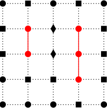
(a) Unstable configuration

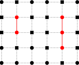
(b) Stable configuration

Figure 5: (a) One can check in this example that (25) implies the non-stability of the configuration for well chosen parameters. Red dots indicates cells with $a_{i}\neq 0$. (b) One can check in this example that (26) is satisfied, ensuring the stability of the configuration.

Next, the reader can verify, using Proposition 7.5, that any patch composed of building blocks disposed in such a way that

$$\partial\Big{(}\partial J_{p}\cup J_{p}\Big{)}\cap\Big{(}\cup_{p^{\prime}\neq p}J_{p^{\prime}}\Big{)}=\emptyset,\ \forall p=1,\cdots,P,$$ (26)

is stable. Figure 5(b) exhibits a typical example of a stable configuration in this setting.

7.4 Example: the pure transport process on the circle

We here assume that $D=0$ and $T=1$. Corollary 7.3 yields the instability of uniform solution $(\rho)=(\rho,\ldots,\rho)$ when the length $L$ of the cycle is larger than 4. The adjacency matrix of the circle is circulant, with eigenvalues given by

$$\mu_{k}=e^{2\pi i\frac{k}{L}}+e^{2\pi i\frac{(L-1)k}{L}}=2\cos\left(2\pi\frac{k}{L}\right).$$

The determinant of $\Gamma$ vanishes if and only if there exists $j\in\{1,...,L\}$ such that $\mu_{j}=0$, that is if

$$\cos\left(2\pi\frac{j}{L}\right)=0\Leftrightarrow 2\pi\frac{j}{L}=\frac{\pi}{2}+k\pi\text{ for }k\in\mathbb{N},$$

or equivalently if there is a $k\in\mathbb{N}$ such that $j=\frac{L}{4}+k\frac{L}{2}\in\mathbb{N}$. Hence, the determinant of $\Gamma$ vanishes if and only if $L$ is a multiple of 4. In this case, the set $M_{c}$ of critical values ${\boldsymbol{a}}$ (that is satisfying $\Gamma{\boldsymbol{a}}=c{\boldsymbol{1}}$) such that $a_{i}>0$, $\forall i\in\Lambda$, is such that

$$a_{3}=c-a_{1},a_{4}=c-a_{2},a_{5}=a_{1},a_{6}=a_{2},a_{7}=c-a_{1},...$$

with $a_{1}\neq 0\neq a_{2}$. Recalling that we impose the following normalization $\sum_{i=1}^{L}a_{i}=\rho L$, we obtain

$$\sum_{i=1}^{L}a_{i}=\rho L\Leftrightarrow 2c\frac{L}{4}=\rho L\Leftrightarrow c=2\rho.$$

The set of critical values $M_{c}$ is then composed of configurations of the form

$${\boldsymbol{a}}=(a_{1},a_{2},2\rho-a_{1},2\rho-a_{2},a_{1},a_{2},2\rho-a_{1},2\rho-a_{2},...,a_{1},a_{2},2\rho-a_{1},2\rho-a_{2})$$

with $(a_{1},a_{2})\in(0,2\rho)\times(0,2\rho)$. Corollary 7.3 then implies that this set contains only unstable points when $L>4$. For $L=4$, the critical point ${\boldsymbol{a}}=(a_{1},a_{2},2\rho-a_{1},2\rho-a_{2})$ is stable since the eigenvalues of the Jacobian matrix are such that

$$\lambda_{1}=\lambda_{2}=\lambda_{3}=0\text{ and }\lambda_{4}=-\frac{2c}{(\kappa+c)^{2}}$$

We can summarize these results in the following corollary:

Corollary 7.7

Assume that the nodes are arranged on a circle of size $L$. The set $M_{c}$ of critical values ${\boldsymbol{a}}>0$ such that $f({\boldsymbol{a}})=0$ contains only the uniform configuration $(\rho,...,\rho)$ if L is not a multiple of 4. In the case where $L=4n$, for some $n\in\mathbb{N}$ with $n\geq 1$, $M_{c}$ is given by

$$M_{c}=\{(a_{1},a_{2},-a_{1}+2\rho,-a_{2}+2\rho,a_{1},a_{2},-a_{1}+2\rho,-a_{2}+2\rho,\cdots);\ a_{k}\in(0,2\rho),\ k=1,2\}.$$

Any element of $M_{c}$ is unstable except for $L=4$.

The set $M_{c}^{tot}$ of all critical points is obtained by decomposing the circle into sub-graph $\gamma$ such ${\boldsymbol{a}}|_{\gamma}>0$ and by solving the system

$$\Gamma_{\gamma}{\boldsymbol{a}}|_{\gamma}=c_{\gamma}{\rm\bf 1}|_{\gamma},$$

for these sub-graphs. We can prove that this system has positive solution ${\boldsymbol{a}}|_{\gamma}$ if and only $|I|<4$ ($|I|:=$ length of the path), because for $|I|\geq 4$, we see that $a_{4}=0$ (which is in contradiction with the hypothesis). When $|I|=3$, the critical points take the form ${\boldsymbol{a}}|_{\gamma}=(z_{1},c_{\gamma},c_{\gamma}-z_{1})$, with $z_{1}\in(0,c_{\gamma})$ and when $|I|=2$, ${\boldsymbol{a}}|_{\gamma}=(c_{\gamma},c_{\gamma})$. In these two cases, the critical points are stable as the Lyapunov function H defined in (18) takes its minimal value $H(a)=-(\kappa+\frac{\rho L}{4})\rho L$. The global minimum of H is obtained by adapting the result of Motzkin and Straus, (1965), see Remark 6.5. Finally, if $|I|=1$, we have ${\boldsymbol{a}}|_{\gamma}=(c_{\gamma})$; $H$ is maximal and hence ${\boldsymbol{a}}$ is unstable.

The set $M_{c}^{tot}$ of critical points is then obtained by taking the direct product of the sets of critical values associated with the paths $\gamma$. For example, if L is a multiple of 4, the subset of $M_{c}^{tot}$ defined by

$$\tilde{M}_{c}=\{(a_{1},a_{2},-a_{1}+2\rho,-a_{2}+2\rho,a_{1},a_{2},-a_{1}+2\rho,-a_{2}+2\rho,\cdots);\ a_{1}=0,\ a_{2}\in(0,2\rho)\},$$

is composed of critical values which are stable since

$$\lambda=0\text{ with multiplicity }3\frac{L}{4}\text{ and }\lambda=\frac{-2c^{2}}{(\kappa+c)^{2}}\text{ with multiplicity }\frac{L}{4}$$

7.5 An explicit computation when $D=0$ on the circle

As we have seen, when $|I|=3$, the stable configurations are given by triplets of the form $(z_{1},c_{\gamma},c_{\gamma}-z_{1})$, where $z_{1}$ is such that $z_{1}\in(0,c_{\gamma})$, for some positive constant $c_{\gamma}>0$.

Consider a path composed of five cells $i-1$, $i$, $i+1$, $i+2$ and $i+3$ such that $a_{i-1}=a_{i+3}=0$, so that the dynamical system (2) associated with these cells becomes

$$\frac{{\rm d}a_{i}}{{\rm d}t} = \frac{a_{i+1}a_{i}}{\kappa+a_{i}+a_{i+2}}-\frac{a_{i}a_{i+1}}{\kappa+a_{i+1}},$$ (27)

$$\frac{{\rm d}a_{i+2}}{{\rm d}t} = \frac{a_{i+1}a_{i+2}}{\kappa+a_{i}+a_{i+2}}-\frac{a_{i+2}a_{i+1}}{\kappa+a_{i+1}},$$ (28)

$$\frac{{\rm d}a_{i+1}}{{\rm d}t} = \frac{a_{i}a_{i+1}}{\kappa+a_{i+1}}+\frac{a_{i+2}a_{i+1}}{\kappa+a_{i+1}}-\frac{a_{i+1}a_{i}}{\kappa+a_{i}+a_{i+2}}-\frac{a_{i+1}a_{i+2}}{\kappa+a_{i}+a_{i+2}}.$$ (29)

Dividing (27) by (28) yields that

$$\frac{\frac{{\rm d}a_{i}}{{\rm d}t}}{\frac{{\rm d}a_{i+2}}{{\rm d}t}}=\frac{a_{i}}{a_{i+2}}.$$

Thus there is a positive constant $c>0$ such that

$$a_{i+2}=ca_{i}.$$ (30)

Plugging this identity in (29), one obtains

$$\frac{{\rm d}a_{i+1}}{{\rm d}t}=(1+c)a_{i}a_{i+1}(\frac{1}{\kappa+a_{i+1}}-\frac{1}{\kappa+a_{i}+a_{i+2}}),$$

and finally

$$\frac{\frac{{\rm d}a_{i+1}}{{\rm d}t}}{\frac{{\rm d}a_{i}}{{\rm d}t}}=-(1+c).$$

Hence there exists a constant $d$ such that $a_{i+1}=d-(1+c)a_{i}$. Normalizing the total mass in such a way that $a_{i}+a_{i+1}+a_{i+2}=3\rho$, one gets that $3\rho=d$ and

$$a_{i+1}=3\rho-(1+c)a_{i}.$$ (31)

Plugging (30) and (31) in equation (27) yields the differential equation

$$\frac{{\rm d}a_{i}}{{\rm d}t}=\frac{a_{i}(3\rho-(1+c)a_{i})(3\rho-2(1+c)a_{i})}{(\kappa+a_{i}(1+c))(3\rho+\kappa-(1+c)a_{i})}.$$

Setting $u=(1+c)a_{i}$, one gets the o.d.e.

$$\frac{{\rm d}u}{{\rm d}t}=\frac{u(3\rho-u)(3\rho-2u)}{(\kappa+u)(3\rho+\kappa-u)}.$$

Solving by partial fractions expansions, one obtains

$$\frac{3\kappa\rho+\kappa^{2}}{9\rho^{2}}(\ln(u)+\ln(3\rho-u))-\frac{9\rho^{2}+4(\kappa^{2}+3\rho\kappa)}{18\rho^{2}}\ln(3\rho-2u)=t+\alpha,$$

for some constant $\alpha$. Clearly one must have $u<3\rho/2$.

Lemma 7.8

As $t\to\infty$, $u(t)=(1+c)a_{i}(t)\longrightarrow\frac{3\rho}{2}$.

Proof.

The preceding considerations show that we have to consider only initial conditions of the form $0\leq u(0)\leq 3\rho$. Clearly $0,\frac{3\rho}{2}$ and $3\rho$ are critical points of our equation.

We can easily find a compact interval $I$ whose interior contains $J=[0,3\rho]$ and so that $f^{\prime}(u)$ is continuous and thus bounded over $I$. As a consequence $f$ satisfies a Lipschitz-condition over $I$. According to the general theory, for any initial condition $u(0)\in J$ our equation admits a unique solution defined over a maximal interval $I_{m}$. If $u(0)=0$, then $u\equiv 0$ is the corresponding solution. If $u(0)\in]0,\frac{3\rho}{2}[$, then $\dot{u}(0)>0$. Due to unicity, the solution can not reach a critical point in a finite time and thus the boundary of $]0,\frac{3\rho}{2}[$. Moreover the solution is obviously bounded entailing $I_{m}=[0,+\infty[$. For the preceding reasons the derivative of $u(t)$ is never $0$ and thus always positive since $\dot{u}(0)>0$. Thus $u(t)$ increases to $\frac{3\rho}{2}$ as $t\rightarrow+\infty$. The same reasoning shows that $u(t)$ decreases to $\frac{3\rho}{2}$ as $t\rightarrow+\infty$ for $u(0)\in]\frac{3\rho}{2},3\rho[$. Finally if $u(0)=3\rho$, then $u\equiv 3\rho$. ∎

Furthermore, (30) yields

$$c=\frac{a_{i+2}(0)}{a_{i}(0)}.$$

As $(1+c)a_{i}=a_{i}+a_{i+2}$ tends to $c_{\gamma}$ as time goes to infinity, Lemma 7.8 yields that $c_{\gamma}=3\rho/2$, and

$$a_{i}(t)\longrightarrow\frac{3\rho}{2(1+c)}=\frac{c_{\gamma}}{1+c},$$

as $t\to\infty$. (30) and (31) show that

$$a_{i+1}=3\rho-(1+c)a_{i}\longrightarrow\frac{3\rho}{2}=c_{\gamma}\text{ and }a_{i+2}=ca_{i}\longrightarrow\frac{c}{1+c}c_{\gamma}=c_{\gamma}-\frac{c_{\gamma}}{1+c}.$$

In summary, one obtains that an orbit defined by initial conditions of the form

$$(a_{i-1}(0),a_{i}(0),a_{i+1}(0),a_{i+2}(0),a_{i+3}(0))\text{ with }a_{i-1}(0)=a_{i+3}(0)=0$$

converges to the critical point $(z_{1},c_{\gamma},c_{\gamma}-z_{1})$, with $z_{1}=\frac{c_{\gamma}}{1+c}$, $c_{\gamma}=\frac{3\rho}{2}$ and ${c=\frac{a_{i+2}(0)}{a_{i}(0)}}$. Finally, if the system starts from a symmetric initial state $a_{i}(0)=a_{i+2}(0)$, the constant c is egal to 1 and the system tends to $(0,\frac{3\rho}{4},\frac{3\rho}{2},\frac{3\rho}{4},0)$ as $t\to\infty$.

8 Appendix

8.1 Proof of Theorem 3.1

First, we easily check that the system $\dot{{\boldsymbol{a}}}=f({\boldsymbol{a}})$ is conservative, i.e.

$$\forall t\in\mathbb{R}_{\geq 0},\;\sum_{i}^{L}a_{i}(t)=\sum_{i}^{L}a_{i}(0).$$

In the following, we use the notation $\dot{{\boldsymbol{a}}}$ instead of $\frac{{\rm d}{\boldsymbol{a}}}{{\rm d}t}$. The latter is equivalent to

$$\sum_{i}^{L}\dot{a}_{i}(t)=\sum_{i}^{L}f_{i}({\boldsymbol{a}})=0.$$

In fact, one can write

$$\sum_{i}\dot{a}_{i}(t) = D\sum_{i}\sum_{k\sim i}(a_{k}-a_{i})+T\sum_{i}\sum_{k\sim i}a_{k}a_{i}\left(\frac{N_{i}-N_{k}}{N_{k}N_{i}}\right)$$

$$= D\sum_{i}(d_{i}a_{i}-d_{i}a_{i})+2T\sum_{k\sim i}\frac{a_{k}a_{i}}{N_{k}N_{i}}((N_{i}-N_{k})-(N_{k}-N_{i}))=0,$$

where $N_{k}=\kappa+\sum_{j\sim k}a_{k}$, and where $d_{i}$ is the degree of i (that is the number of neighbours of i).

Next, system (2) can be written as

$$\dot{a}_{i}=D\sum_{k\sim i}a_{k}+T\sum_{k\sim i}\left(\frac{a_{k}}{\kappa+\sum_{j\sim k}a_{j}}-\frac{a_{k}}{\kappa+\sum_{j\sim i}a_{j}}-\frac{D}{T}\right)a_{i}.$$ (32)

Let ${\boldsymbol{a}}$ a solution of (32) with ${\boldsymbol{a}}(0)\in\mathbb{R}^{L}_{\geq 0}$.

We say that the function $f:\mathbb{R}_{+}\rightarrow\mathbb{R}$ is instantaneously positive (i.p.) if there exists $\delta>0$ so that $f$ is strictly positive over $(0,\delta)$. If $f(0)>0$ and $f$ is continuous to the right at $0$, then $f$ is i.p.. It is also clear that if $f$ admits a strictly positive right-hand derivative at $0$, then it is i.p..

Let $U$ be the open set $U=\{{\boldsymbol{x}}=(x_{1},x_{2},...,x_{L})\in\mathbb{R}^{L};-\frac{\kappa}{2L}<x_{i}\}$. Since the right-hand member of (32) is continous over $U$, the general theory of o.d.e.’s provides the existence of a solution defined over a maximal interval $0\in J^{+}\subset\mathbb{R}_{+}$ for any initial condition ${\boldsymbol{a}}(0)\in U$. Moreover, the solution is unique because the right-hand member of (32) locally lipschitzian. Set for convenience

$$h_{i}(t) = D\sum_{k\sim i}a_{k}(t)\quad\hbox{ and }$$

$$g_{i}(t) = T\sum_{k\sim i}\left(\frac{a_{k}(t)}{\kappa+\sum_{j\sim k}a_{j}(t)}-\frac{a_{k}(t)}{\kappa+\sum_{j\sim i}a_{j}(t)}-\frac{D}{T}\right).$$

The variation of constants formula allows us to write , $\forall t\in J^{+}$,

$$a_{i}(t)=a_{i}(0)e^{\int_{0}^{t}g_{i}(s)ds}+\int_{0}^{t}h_{i}(u)e^{-\int_{u}^{t}g_{i}(v)dv}du.$$ (33)

Since $a_{i}(0)\geq 0$, the first term in (33) is non-negative. Moreover if $a_{k}(t)$ is i.p. for some $k\sim i$, then according to (33), the same property holds for $a_{i}(t)$. In particular, if $a_{k}(0)>0$ for some $k\sim i$, then by continuity $a_{k}(t)$ is i.p. and thus also $a_{i}(t)$.

The case $D>0$:

Clearly, if ${\boldsymbol{a}}(0)={\boldsymbol{0}}$, then the unique solution is identically $0$. Otherwise, there exists $1\leq i_{0}\leq L$ with $a_{i_{0}}(0)>0$ and $\forall j\sim i_{0},a_{j}(t)$ is i.p.. Since our graph is supposed to be connected, every $i$ admits a neighbor $k\sim i$ with $a_{k}(t)$ i.p.. Hence, $a_{i}(t)$ is i.p. $\forall i,1\leq i\leq L$.

The preceding arguments show that for any initial condition ${\boldsymbol{a}}(0)\in\mathbb{R}_{\geq 0}^{L}\subset U$, all components of the solution of (32) are i.p.. Let us suppose that one of them admits the value $0$ in $J^{+}\backslash\{0\}$. Since all components are continuous and their number is finite, there exists a first time $t_{0}>0$ for which at least one component $a_{i_{0}}(t_{0})=0$ and all of them are strictly positive over $(0,t_{0})$. According to (33), we have

$$a_{i_{0}}(t_{0})=0=a_{i}(0)e^{\int_{0}^{t_{0}}g_{i}(s)ds}+\int_{0}^{t_{0}}h_{i}(u)e^{-\int_{u}^{t_{0}}g_{i}(v)dv}du.$$

Clearly $h_{i}(t)>0$ over $J^{+}\backslash\{0\}$ and since the first term is non-negative, we conclude to $a_{i_{0}}(t_{0})>0$, a contradiction. Therefore all $a_{i}(t)$ are strictly positive over $J^{+}\backslash\{0\}$.

The case $D=0$:

If $a_{i}(0)=0$, the homogeneous equation for $a_{i}(t)$ admits only the zero solution, and we remove the related $i$th component from (32). Otherwise $a_{i}(0)>0$ and, by continuity, $a_{i}(t)$ is i.p.. In that case $a_{i}(t)=a_{i}(0)e^{\int_{0}^{t}g_{i}(s)ds}>0$ over $J^{+}$.


In both cases the solution of (32) have strictly positive components over $J^{+}$. We also proved that $\forall t\in J^{+}$ we have:

$$\sum_{1\leq i\leq L}a_{i}(t)=\sum_{1\leq i\leq L}a_{i}(0).$$

As a consequence the solution of (32) is bounded and thus the unique solution of our problem is defined over $J^{+}=[0,+\infty)$.

8.2 Proof of Proposition 7.1

We first give the Jacobian, for general ${\boldsymbol{a}}$. We have

$$\frac{\partial f_{i}({\boldsymbol{a}})}{\partial a_{j}}=\frac{a_{i}}{N_{j}}-\frac{a_{i}}{N_{i}}+\sum_{k\sim i}\frac{a_{i}a_{k}}{N_{i}^{2}}-\sum_{k\sim i,k\sim j}a_{k}\frac{a_{i}}{N_{k}^{2}},$$ (34)

(where the last term is due to the triangles in the graph) when $j\sim i$, that is, $i$ and $j$ are nearest neighbours. When $i=j$, one gets

$$\frac{\partial f_{i}({\boldsymbol{a}})}{\partial a_{i}}=\sum_{k\sim i}\frac{a_{k}}{N_{k}}-a_{i}\sum_{k\sim i}\frac{a_{k}}{N_{k}^{2}}-\frac{\sum_{k\sim i}a_{k}}{N_{i}}.$$ (35)

The remaining non-vanishing partial derivatives correspond to nodes $j$ located at distance 2 of $i$ in the graph, that is, to nodes $j$ such that $j\sim k$ for some $k\sim i$, $j\neq i$ but $i\not\sim j$. Then

$$\frac{\partial f_{i}({\boldsymbol{a}})}{\partial a_{j}}=-\sum_{j\sim k,\ k\sim i}\frac{a_{i}a_{k}}{N_{k}^{2}}.$$ (36)

When $N_{i}=N$, $\forall i$, these expressions simplify to

$$\frac{\partial f_{i}({\boldsymbol{a}})}{\partial a_{j}}=\sum_{k\sim i}\frac{a_{i}a_{k}}{N_{i}^{2}}=\frac{N-\kappa}{N^{2}}a_{i}-\frac{a_{i}}{N^{2}}\sum_{k\sim i,k\sim j}a_{k}.$$

If $j\sim i$,

$$\frac{\partial f_{i}({\boldsymbol{a}})}{\partial a_{i}}=-\frac{N-\kappa}{N^{2}}a_{i},$$

and

$$\frac{\partial f_{i}({\boldsymbol{a}})}{\partial a_{j}}=-\sum_{k\sim i,k\sim j}\frac{a_{i}a_{k}}{N_{k}^{2}}=-\frac{a_{i}}{N^{2}}\sum_{k\sim i,k\sim j}a_{k},$$

if $j\sim k$ for some $k\sim i$, $j\neq i$ but $i\not\sim j$.
Consider the sub-matrix $L$ given by $L=(\partial f_{i}({\boldsymbol{a}})/\partial a_{j})_{j\sim i}$. Let $d({\boldsymbol{a}})$ be the diagonal matrix of diagonal given by ${\boldsymbol{a}}$. The perturbation associated with the triangles contained in the graph is represented by the term $-\frac{a_{i}}{N^{2}}\sum_{k\sim i,k\sim j}a_{k}$ in $\frac{\partial f_{i}({\boldsymbol{a}})}{\partial a_{j}}$ for $j\sim i$, and the related matrix is given by

$$\left(-\frac{a_{i}}{N^{2}}\sum_{k\sim i,k\sim j}a_{k}\right)\gamma_{ij} = \left(-\frac{a_{i}}{N^{2}}\sum_{k}\gamma_{ik}a_{k}\gamma_{kj}\right)\gamma_{ij}$$

$$= \left(-\frac{1}{N^{2}}\left(d(a)\Gamma d(a)\Gamma-{\rm diag}(d(a)\Gamma d(a)\Gamma)\right)_{ij}\right)\gamma_{ij}$$

$$= \left(-\frac{1}{N^{2}}(d(a)\Gamma d(a)\Gamma)_{ij}+\frac{N-\kappa}{N^{2}}d(a)_{ij}\right)\gamma_{ij}.$$

The matrix $L$ is now given by

$$L=\frac{d(a)}{N^{2}}(N-\kappa)(\Gamma-id)-\frac{1}{N^{2}}(d(a)\Gamma d(a)\Gamma-(N-\kappa)d(a))\circ\Gamma,$$

where $\circ$ represents the Hadamard product, i.e. the multiplication component by component.
Likewise, the perturbation of $L$ by $\left(\frac{\partial f_{i}({\boldsymbol{a}})}{\partial a_{j}}\right)_{i\sim k,k\sim j,i\not\sim j,i\neq j}$ can be written as

$$\left(-\frac{a_{i}}{N^{2}}\sum_{\begin{subarray}{c}k\sim i,k\sim j,\\ i\not\sim j,i\neq j\end{subarray}}a_{k}\right)\gamma_{ij} = \left(-\frac{a_{i}}{N^{2}}\sum_{k}\gamma_{ik}a_{k}\gamma_{kj}\right)(1-\gamma_{ij}-id_{ij})$$

$$= \left(-\frac{1}{N^{2}}(d(a)\Gamma d(a)\Gamma)_{ij}+\frac{N-\kappa}{N^{2}}d(a)_{ij}\right)(1-\gamma_{ij}-id_{ij}).$$

The related Jacobian is thus given by $L+\left(\frac{\partial f_{i}({\boldsymbol{a}})}{\partial a_{j}}\right)_{i\sim k,k\sim j,i\not\sim j,i\neq j}$, that is

$$df(a) = \frac{d(a)}{N^{2}}(N-\kappa)(\Gamma-id)-\frac{1}{N^{2}}(d(a)\Gamma d(a)\Gamma-(N-\kappa)d(a))\circ\Gamma$$

$$-\frac{1}{N^{2}}(d(a)\Gamma d(a)\Gamma-(N-\kappa)d(a))\circ(\mathbb{1}-\Gamma-id)$$

$$= \frac{d(a)}{N^{2}}(N-\kappa)(\Gamma-id)-\frac{1}{N^{2}}(d(a)\Gamma d(a)\Gamma-(N-\kappa)d(a))\circ(\mathbb{1}-id)$$

$$= \frac{d(a)}{N^{2}}(N-\kappa)(\Gamma-id)-\frac{1}{N^{2}}(d(a)\Gamma d(a)\Gamma-(N-\kappa)d(a)),$$

where $\mathbb{1}$ is the matrix composed only of ones. The last equality is a consequence of the fact that the diagonal of $d(a)\Gamma d(a)\Gamma-(N-\kappa)d(a)$ vanishes. Hence,

$$df(a)=\frac{d(a)\Gamma}{N^{2}}((N-\kappa)id-d(a)\Gamma)=\frac{d(a)\Gamma}{N^{2}}(c\ id-d(a)\Gamma),$$

proving the result.

8.3 Proof of Proposition 7.5

Set $I=\{i\in\Lambda:a_{i}=0\}$, and consider the sub-graphs $\gamma_{p}$ of $G$ induced by the nodes of $J=\Lambda\setminus I$, with $\gamma_{p}=(\Lambda_{p},E_{p})$, $1\leq p\leq P$. The related critical points ${\boldsymbol{a}}$ are such that the restrictions ${\boldsymbol{a}}|_{\gamma_{p}}$ satisfy the linear systems $\Gamma_{\gamma_{p}}{\boldsymbol{a}}|_{\gamma_{p}}=c_{\gamma_{p}}{\boldsymbol{1}}|_{\gamma_{p}}$. Set $N_{\gamma_{p}}=c_{\gamma_{p}}+\kappa$.

(34) - (36) permit to compute the entries of the Jacobian matrix, by first looking at the diagonal entries: When $i\in\Lambda_{p}$, one has

$$\frac{\partial f_{i}({\boldsymbol{a}})}{\partial a_{i}}=-a_{i}\frac{N_{\gamma_{p}}-\kappa}{N_{\gamma_{p}}^{2}},$$

providing the diagonal entry of the Jacobian of $f|_{\gamma_{p}}({\boldsymbol{a}}|_{\gamma_{p}})$. When $i\not\in\Lambda_{p}$, a similar computation yields

$$\frac{\partial f_{i}({\boldsymbol{a}})}{\partial a_{i}}=\sum_{k\sim i}\frac{a_{k}}{N_{k}}-\frac{N_{i}-\kappa}{N_{i}}.$$

We then compute the entries $(i,j)$ for $j\sim i$:

$$\frac{\partial f_{i}({\boldsymbol{a}})}{\partial a_{j}}=a_{i}\frac{N_{\gamma_{p}}-\kappa}{N_{\gamma_{p}}^{2}}-\sum_{k\sim i,k\sim j}a_{k}\frac{a_{i}}{N_{k}^{2}}=a_{i}\frac{N_{\gamma_{p}}-\kappa}{N_{\gamma_{p}}^{2}}-\sum_{k\sim i,k\sim j,k\in\Lambda_{p}}\frac{a_{k}a_{i}}{N_{\gamma_{p}}^{2}},$$

for $i,j\in\Lambda_{p}$ and $1\leq p\leq P$, which corresponds to the $(i,j)$ entry of the Jacobian of $f|_{\gamma_{p}}({\boldsymbol{a}}|_{\gamma_{p}})$. Likewise,

$$\frac{\partial f_{i}({\boldsymbol{a}})}{\partial a_{j}}=\frac{a_{i}}{N_{j}}-\frac{a_{i}}{N_{\gamma_{p}}}+\sum_{k\sim i}\frac{a_{i}a_{k}}{N_{\gamma_{p}}^{2}}-\sum_{\begin{subarray}{c}k\sim i,k\sim j,\\ k\in\Lambda_{p}\end{subarray}}\frac{a_{k}a_{i}}{N_{\gamma_{p}}^{2}}=\frac{a_{i}}{N_{j}}-a_{i}\frac{\kappa}{N_{\gamma_{p}}^{2}}-\frac{a_{i}}{N_{\gamma_{p}}^{2}}\sum_{\begin{subarray}{c}k\sim i,k\sim j,\\ k\in\Lambda_{p}\end{subarray}}a_{k},$$

when $i\in\Lambda_{p}$ for some $p$ and $j\not\in\Lambda_{p}$. Finally,

$$\frac{\partial f_{i}({\boldsymbol{a}})}{\partial a_{j}}=0,$$

when $i,j\not\in\cup_{p}\Lambda_{p}$, or equivalently when both $i$ and $j$ belongs to $I$.

We next consider $(i,j)$ entries where $j$ is at a distance 2 of $i$ in the graph $G$, that is when $j$ is such that $j\sim k$ for some $k\sim i$, $j\neq i$ and $j\not\sim i$. One obtains that

$$\frac{\partial f_{i}({\boldsymbol{a}})}{\partial a_{j}}=-a_{i}\sum_{j\sim k,k\sim i}\frac{a_{k}}{N_{\gamma_{p}}^{2}},$$

when $i,j,k\in\Lambda_{p}$, which is the $(i,j)$ entry of the Jacobian of $f|_{\gamma_{p}}({\boldsymbol{a}}|_{\gamma_{p}})$.

Likewise,

$$\frac{\partial f_{i}({\boldsymbol{a}})}{\partial a_{j}}=-a_{i}\sum_{j\sim k,k\sim i}\frac{a_{k}}{N_{\gamma_{p}}^{2}},$$

when $i,k\in\Lambda_{p},j\not\in\Lambda_{p}$ ($\Rightarrow j\in I$).

Next,

$$\frac{\partial f_{i}({\boldsymbol{a}})}{\partial a_{j}}=0.$$

when $i\,\mathrm{or}\,k\not\in\Lambda_{p},\forall j\in\Lambda$.

Permuting conveniently the indices, the Jacobian ${\rm d}f({\boldsymbol{a}})$ can be written as

$${\rm d}f({\boldsymbol{a}})=\begin{pmatrix}d_{n}&{\boldsymbol{0}}\\ \ast&{\rm d}f^{\gamma}\end{pmatrix}$$ (37)

where $d_{n}$ is a diagonal matrix $n\times n$ with entries given by $\lambda_{i}:=\sum_{k\sim i}\frac{a_{k}}{N_{k}}-\frac{N_{i}-\kappa}{N_{i}}$, for $i\in I$, and hence ${\rm d}f^{\gamma}$ is a block diagonal matrix, each block being equal to the Jacobian of $f$ restricted on each sub-graph $\gamma_{p}$. The permutation allows us to group all indices $i\in I$ in the same block, and all indices related to the sub-graphs $\gamma_{p}$ are also arranged together. It follows that the eigenvalues of ${\rm d}f({\boldsymbol{a}})$ are given by the diagonal entries $(\lambda_{i})_{i\in I}$, and by the eigenvalues of all Jacobian matrices.

Acknowledgements This work was supported by the University of Fribourg, and by the SystemsX "Plant growth in changing environments" project funding. Many thanks to D. Kierzkowski and C. Kuhlemeier for providing us the picture given in Figure 1 and to Aleš Janka for its help in Matlab programming. We are very grateful to Patrick Favre and Didier Reinhardt for giving us the opportunity to learn parts of the actual knowledge on the role of the auxin flux in plant patterning.

References

- Adler, (1974) Adler I (1974) A Model of Contact Pressure in Phyllotaxis. J. Theor. Biol. 1:1–79.
- Atela et al., (2002) Atela P, Golé C, Hotton C (2002) A dynamical system for plant pattern formation. J. Nonlin. Sci 12:641–676.
- Barbier de Reuille et al., (2006) Barbier de Reuille P, Bohn-Courseau I, Ljung K, Morin H, Carraro N, Godin C, Traas J (2006) Computer Simulations Reveal Properties of the Cell-cell Signaling Network At the Shoot Apex in Arabidopsis. Proc. Natl. Acad. Sci. USA 103:1627–1632.
- Bayer et al., (2009) Bayer E, Smith R, Mandel T, Nakayama N, Sauer M, Prusinkiewicz P, Kuhlemeier C (2009) Integration of Transport-based Models for Phyllotaxis and Midvein Formation. Genes and Development 23:373–384.
- Benaïm, (1997) Benaïm M (1997) Vertex-reinforced Random Walks and a Conjecture of Pemantle. Ann. Prob. 25:361–392.
- Benaïm and Tarrès, (2008) Benaïm M and Tarrès P (2008) Dynamics of Vertex-Reinforced Random Walks. ArXiv e-prints 0809.2739v3.
- Boudaoud, (2010) Boudaoud A (2010) An Introduction to the Mechanics of Morphogenesis for Plant Biologists. Trends in Plant Science 15:353–360.
- Diaconis and Stroock, (1991) Diaconis P, Stroock D (1991) Geometric Bounds for Eigenvalues of Markov Chains. Ann. Appl. Proba. 1:36–61.
- Douady and Couder, (1996) Douady S, Couder Y (1996) Phyllotaxis As a Dynamical Self Organizing Process (Part I, II, III). J. Theor. Biol. 178:255–312.
- Dumais, (2007) Dumais J (2007) Can mechanics control pattern in plants ? Current Opinion in Plant Biology 10:58–62.
- Dumais and Steele, (2000) Dumais J, Steele C (2000) New Evidence for the Role of Mechanical Forces in the Shoot Apex Meristem. Journal of Plant Growth Regulation 19:7–18.
- Ethier and Kurtz, (1986) Ethier SN, Kurtz TG (1986) Markov processes: characterization and convergence. Wiley series in probability and mathematical statistics.
- Evans et al., (2006) Evans, M., Hanney, T. and Majumdar, S. (2006) Interaction-Driven Real-Space Condensation. Physical Review Letters 97:010603.
- Gabriel et al., (1989) Gabriel JP, Hanisch H, Hirsch W (1988-1989) Prepatency and sexuality of parasitic worms : the hermaphroditic case. Atti del colloquio di matematica, Edizione Cerfim Locarno, Anno 3, vol 4.
- Green, (1980) Green P (1980) Organogenesis- a Biophysical View. Annual Review of Plant Physiology 31:51–82.
- Grosskinsky et al., (2011) Grosskinsky S, Redig F, Vafayi K (2011) Condensation in the Inclusion Process and Related Models. J. Stat. Phys. 142:952–974.
- Hamant et al., (2008) Hamant O, Heisler MG, Jönsson H, Krupinski P, Uytterwaal M, Bokov P, Corson F, Sahlin P, Boudaoud A, Meyerowitz E, Couder Y, Traas J (2008) Developmental Patterning by Mechanical Signals in Arabidopsis. Science 322:1650–1655.
- Hamant and Traas, (2009) Hamant O, Traas J (2009) The Mechanics Behind Plant Development. New Phytologist 185:369–385.
- Heisler, (2006) Heisler MG, Jönsson H (2006) Modeling Auxin Transport and Plant Development. J. Plant Growth Regul. 25:302–312.
- Hofmeister, (1868) Hofmeister W (1868) Handbuch der Physiologischen Botanik: Allgemeine Morphologie der Gewächse, 405–664. Engelmann, Leipzig.
- Jönsson et al., (2006) Jönsson H, Heisler MG, Shapiro BE, Mjolsness E, Meyerowitz EM (2006) An Auxin-driven Polarized Transport Model for Phyllotaxis. Proc. Natl. Acad. Sci. USA , 103:1633–1638.
- Kipnis and Landim, (1999) Kipnis C, Landim C (1999) Scaling limits of interacting particle systems, vol. 320, of Grundlehren der Mathematischen Wissenschaften [Fundamental Principles of Mathematical Sciences]. Springer-Verlag, Berlin.
- Kunz, (1995) Kunz M (1995) Some Analytical Results About Two Physical Models of Phyllotaxis. Commun. Math. Phys. 169:261–295.
- LaSalle, (1976) LaSalle JP (1976) The stability of dynamical systems. SIAM, Philadelphia.
- Levitov, (1991) Levitov LS (1991) Energetics Approach to Phyllotaxis. Europhys. Lett. 14:533–539.
- Luck and Godrèche, (2007) Luck JM, Godrèche C (2007) Structure of the stationary state of the asymmetric target process. J. Stat. Mech. Theory Exp. P08005 (electronic).
- Meinhardt, (1982) Meinhardt H (1982) Models of Biological Pattern Formation. Academic Press.
- Mjolsness, (2006) Mjolsness E (2006) The Growth and Development of some Recent Plant Models: a Viewpoint. J. Plant Growth Regul. 25:270–277
- Motzkin and Straus, (1965) Motzkin T, Straus G (1965) Maxima for Graphs a New Proof of a Theorem of Turán. Canad. J. Math. 17:533–540.
- Newell and Shipman, (2005) Newell A, Shipman P (2005) Plant and Fibonacci. J. Stat. Phys. 121:937–968.
- Newell et al., (2008) Newell AC, Shipman PD, Sun Z (2008) Phyllotaxis: Cooperation and Competition Between Mechanical and Biochemical Processes. Journal of Theor. Biol. 251:421–439.
- Pemantle, (1992) Pemantle R (1992) Vertex-reinforced random walk. Probab. Theory Related Fields 92:117–136.
- Reinhardt et al., (2000) Reinhardt D, Mandel T, Kuhlemeier C (2000) Auxin Regulates the Initiation and Radial Position of Lateral Organs. Plant Cell 12:501–518.
- Reinhardt et al., (2003) Reinhardt D, Pesce E, Stieger P, Mandel T, Baltensperger K, Bennett M, Traas J, Friml J, Kuhlemeier C (2003) Regulation of Phyllotaxis by Polar Auxin Transport. Nature 426:255–260.
- Reinhardt et al., (2005) Reinhardt D (2005) Phyllotaxis - a new chapter in an old tale about beauty and magic numbers. Current Opinion in Plant Biology 8:487–493.
- Sahlin et al., (2009) Sahlin P, Söderberg B, Jönsson H (2009) Regulated transport as a mechanism for pattern generation : Capabilities for phyllotaxis and beyond. Journal of Theoretical Biology 258:60–70.
- Scarpella et al., (2006) Scarpella E, Marcos D, Friml J, Berleth T (2006) Control of Leaf Vascular Patterning by Polar Auxin Transport. Genes Dev. 20:1015–1017.
- Shipman and Newell, (2005) Shipman PD, Newell AC (2005) Polygonal Plantform and Phyllotaxis on Plants. Journal of Theor. Biol. 236:154–197.
- Smith et al., (2006) Smith RS, Guyomarch’s S, Mandel T, Reinhardt D, Kuhlemeier C et al. (2006) A Plausible Model of Phyllotaxis. Proc. Natl. Acad. Sci. USA 103:1301–1306.
- Thornley, (1975) Thornley J (1975) Phyllotaxis I. A mechanistic model. Annals of Botany 39:491–507.
- Turing, (1952) Turing A (1952) The Chemical Basis of Morphogenesis. Philo. Trans. Roy. Soc. London 237:37–72.
- Waller, (1977) Waller D (1977) Optimisation of Quadratic Forms Associated with Graphs. Glasgow Math. J. 18:79–85.