Stellar velocity dispersion of Luminous Compact Galaxies at intermediate redshift

Abstract

We present the stellar velocity dispersion measurements for 5 Luminous Compact Galaxies (LCGs) at z=0.5-0.7. These galaxies are vigorously forming stars with average SFR $\sim$ 40 M_⊙/yr. We find that their velocity dispersions range from $\sim 137\ \rm{km/s}$ to $260\ \rm{km/s}$, while their stellar masses range between $4\times 10^{9}$ and $10^{11}$ M_⊙. If these LCGs evolve passively after this major burst of star formation, their masses and velocity dispersions, as well as their evolved colours and luminosities are most consistent with the values characteristic of early-type spiral galaxies today.

1 Introduction

Luminous Compact Galaxies (Hammer et al., 2001) are starbursts galaxies at intermediate redshifts mostly detected in both UV and IR wavelengths, characterised by having small effective radii ($R_{e}<5\ \rm{kpc}$), high luminosities ($M_{AB}(B)\leqslant-20$) and strong emission lines. Hammer et al. (2001) observed a representative sample of LCGs selected from the CFRS fields using the intermediate resolution ($R>600$) spectrograph FORS1 and FORS2 on the VLT/Kuyen telescope. The spectra revealed some strong absorption lines (Ca II K and H, G Band, Fe I, and Balmer lines) as well as narrow and intense emission lines ([OII]$\lambda 3727$Å, [OIII]$\lambda\lambda 4858,5007$ÅÅ, Balmer lines). The spectro-photometric analysis of these galaxies (Hammer et al. 2001, Gruel 2002) showed that they are likely composed of three different stellar populations. The youngest population presents strong emission lines ([OII]$\lambda 3727$Å  Balmer lines), indicating present day active star formation and sub-solar metallicity. A second stellar population was formed within the last few hundred million years. It is characterised by a solar metallicity and the presence of Balmer lines in absorption. The third stellar population, older than 5 Gyr, exhibits solar metal abundances and strong metallic absorption lines (Calcium, Iron lines, G band, Titanium, etc.) (Gruel, 2002).

Almost all LCGs analysed by Hammer et al. (2001) have large extinction coefficients ($A_{v}\sim 1.5$), yielding average extinction-corrected star formation rates SFR $\sim 40\rm{M}_{\odot}\,\rm{yr}^{-1}$ (which is $\sim$10 times higher than those estimated from the UV fluxes) (Hammer et al. 2001, Gruel 2002). Some LCGs show morphological irregularities and/or close companions as revealed in HST images (Hammer et al. 2001, Zheng et al. 2004). These observations suggest that LCGs may be undergoing violent star formation events similar to those occurring in close interacting systems. Hammer et al. (2001) concluded that these LCGs may be the progenitors of the bulges of spirals galaxies forming inside-out.

A new parameter to shed light on LCGs local counterparts is the galaxy’s kinematics. Measurements of the $H\beta$ emission line velocity widths for Hammer et al. LCG sample showed low velocity widths of $\sim 70$ km^-1, suggesting they may be low mass objects ($\sim 10^{9}$M_⊙). $H\alpha$ velocity widths for a handful LCGs measured with ISAAC at the VLT (Tresse et al., 2002), showed a “double horn” profile characteristic of rotation. Integral spectroscopy was also used to measure the velocity field for some LCGs by Puech et al. (2006) using GIRAFFE at the VLT. However, due to the small apparent size of these objects, the velocity map extends only over very few spaxels.

The most reliable measurement of galaxy kinematics is the stellar velocity dispersion from absorption lines. In this paper, we present the first velocity dispersion measurements from absorption lines for 5 LCGs at intermediate redshift. We constrain our study to the spectral range that includes the Balmer lines ($H10,H9,H8,H\epsilon,H\delta,H\gamma$), the calcium doublet $\rm{Ca}II\ K$,$H$ and the G Band. Section 2 presents the data set for our galaxy sample. Section 3 describes the methods used to measure the velocity dispersion, the photometry and the stellar masses of these galaxies. Section 4 contains the results and the discussion. We assume the following cosmology in this paper: $\textrm{H}_{0}=70\textrm{ km s}^{-1}\textrm{ Mpc}^{-1}$, $\Omega_{\lambda}=0.7$ and $\Omega_{m}=0.3$.

2 Data

2.1 Sample selection

The galaxy sample was selected from three Canada France Redshift Survey (CFRS) fields: CFRS 0000+00 (Le Fevre et al., 1995), CFRS 0300+00 (Hammer et al., 1995) and CFRS 2230+00 (Lilly et al., 1995). Intermediate-z LCGs were selected using criteria defined by Hammer et al. (2001): size ($r_{1/2}\leqslant 5\,\textrm{h}^{-1}_{50}\ \textrm{kpc}$), luminosity ($M_{AB}(B)\leqslant-20.0$), redshift ($0.5\leqslant z\leqslant 1$) and the presence of a major star formation episode characterised by an [OII]$\lambda 3727$Å emission with an equivalent width $EW([OII]\lambda 3727$Å$)\geqslant 15$Å. This results in a sample of 32 LCGs, or 29% of the most luminous ($M_{AB}(B)\leqslant-20.0$) galaxies found in the three CFRS fields (Gruel 2002). We observed 22 of these galaxies with the FORS/R600 and I600 spectrograph at the European Southern Observatory 8m VLT/Kueyen at a resolution of FWHM=5 Å (Hammer et al. 2001, Gruel 2002). The typical exposure times were 12000 seconds per object.

We reduced the spectroscopic data by using the Multired package within IRAF. Measurements and analysis (flux, equivalent width, star absorption correction, metallicity) were done with software described in Gruel (2002).

In this paper, we analyse a subsample of give LCGs with the higest S/N and the strongest absorption lines, for which measurements of stellar velocity dispersion are feasible.

3 Methods

3.1 Velocity dispersion measurements from the absorption lines

Velocity dispersion was measured with the program Movel, included in the REDUCEME softwares package (Cardiel et al., 1998). The instrumental resolution of our LCG sample is FWHM$\sim 5$ Å ($\sigma_{ins}\sim 100\ km/s$). The lowest velocity dispersion measurable with this instrumental resolution is $\sigma\sim 70\ \rm{km/s}$ for spectra with $S/N>10$ (Matković & Guzmán 2005). We thus selected galaxies from our LCGs sub-sample with $S/N\ga 10$ per resolution element. The S/N criteria reduced the LCGs sample to only 5 objects. The final sample is given in table 2.

Since the original aim of the observations was to analyse emission lines, we did not observe stars that we could use as templates. Therefore, we created our own a series of stellar templates with the same instrumental resolution as the LCGs.

We used stellar templates from MILES spectral stellar library (Sánchez-Blázquez et al. 2006, Falcón-Barroso et al. 2011), which includes stars observed between July 2001 and December 2002 in La Palma (Spain) at the Isaac Newton telescope. These templates are the basis of our galaxy template. Since their resolution is higher ($\sim 2.5$Å FWHM) than our sample of galaxies (R=600), we convolved them with a gaussian kernel. The characteristics of the gaussians used for the convolution was determined from the difference between the instrumental resolution of the galaxies and the stellar database. The instrumental/spectral resolution of the individual LCGs was determined from the sky spectrum obtained with the same slit as the spectrum of the galaxy. The intrinsic dispersion of the instrument is given by $\sigma_{Inst}=\frac{\rm{FWHM_{sky}}}{2.35}\times\frac{1}{\lambda}\times c$. The value of the Gaussian function used to broaden the stellar template is the quadratic difference of the instrumental resolution of our observations and that of the stellar library: $\Delta\sigma=\sqrt{\sigma_{Inst}^{2}-\sigma_{stars}^{2}}$ (See Fig. 1).

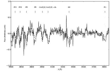
Figure 1: Example of one stellar spectrum (22.0637) (plain line) with the best broadened stellar template fit (dashed line) obtained with Movel. The different absorption lines used are labelled.

Using a stellar database to build stellar templates by convolving the instrumental resolution to one’s own observations has already been successfully demonstrated for early-type galaxies by Treu et al. (1999), Treu et al. (2001a), Treu et al. (2001b). The studies proved that at any given S/N and resolution, there is a lower limit to the velocity dispersion that can be measured. Typically, this limit stands at half the instrumental resolution of a given galaxy spectrum at low S/N (Bender, Burstein, & Faber, 1992). All measurements with a $S/N<10$ per resolution element are deemed not reliable. Treu et al. (2001a) and Matković & Guzmán (2005) quantified the errors for different S/N and range of velocity and showed that the systematic error for a galaxy with a S/N$\ga 10$ and a velocity dispersion of 150 km/s is $\sim 15$%.

Velocity dispersions for the galaxies were measured using the MOVEL and OPTEMA algorithms described by Gonzalez (1993). The MOVEL algorithm is an iterative procedure based in the Fourier Quotient method (Sargent et al. 1977) in which a galaxy model is processed in parallel to the galaxy spectrum. The main improvement of the procedure is introduced through the OPTEMA algorithm, which is able to overcome the typical template mismatch problem by constructing for each galaxy an optimal template as a linear combination of stellar spectra of different spectral types and luminosity classes.

For this study, error in velocity dispersion measurement was statistically determined by bootstrapping. One hundred pseudo-spectra were randomly simulated in the range given by the galaxy error spectrum using a gaussian noise model. The error of the velocity dispersion measurement was obtained from the statistical distribution of the 100 pseudo-spectra measurements.

Different effects limit the precision or the ability to measure galaxy velocity dispersion. Stellar template mismatch is one such limiting factor. This effect happens when the star template used to fit the galaxy spectrum are not representative of the real stellar population of the galaxy. Creating a galaxy template from a stellar library can be impossible, the stellar library does not contains every stellar type and one of the main stellar population which composed the observed galaxy can be missing. As this template is a first guess to start the velocity dispersion measurement, no numerical criteria to avoid template mismatch is used. It is possible to help the software to make this first guess by removing some extra-features (see below) or limiting the number of stars in the library to the one presenting the most important features for velocity dispersion measurement. We removed every galaxy spectrum from our sample when an important template mismatch at the initial step was visually detected even if their S/N was over $10$. To test the impact of a small initial template mismatch (no visual detection and $\chi^{2}$ greater than the template automatically created by the software) we forced the software to use specific templates, thus creating an artificial template mismatch. Measurement of the velocity dispersion with this mismatch showed an error of $\sim 5$% in the dispersion measurement.

In our case, another effect is introduced by the convolution of the instrumental resolution of the stellar templates to that of the LCG’s. The effect of this modification was intensively tested with galaxies of well known velocity dispersion. An elliptical galaxy from the Coma cluster was changed and the velocity dispersion measured with the templates convolved to a slightly different one. The procedure was repeated with a pseudo-instrumental resolution modified up to $\pm 3$Å in 0.05Å steps. An error of $0.1$Å in the difference of resolution introduces an error of 5% in the velocity dispersion measurement. The error in velocity dispersion increases more strongly with higher error in resolution. At $\pm 0.1$Å the error is $\sim 5$%, while at $\pm 0.2$Å and $\pm 0.5$Å the errors are respectively $\sim 10$% and $\sim 22$% in the dispersion measurement. The galaxies instrumental resolution were measured using different lines from the sky spectrum extracted at the same time than the LCG spectra with the same polynomial (Gruel, 2002). The resolution measured from the different lines was stable at $\pm 0.1$Å along the spectrum.

Small emission lines tend to fill the Balmer lines (our major features) changing the global shape of the absorption features To quantify the influence of this contamination, the emission lines in our sample were masked and velocity dispersion was measured without them. We also observed that if not removed entirely, an artifact can appear at the continuum substraction step for the strongest emission lines such as [OII]$\lambda 3727$Å or H$\beta$ and bad sky substraction features. As a result these lines were erased manually. Both effects were quantified (measured with and without the lines) as an error of 2% for the strong emission line $[OII]\lambda 3727$Å and 5% for the emission inside the Balmer lines. For galaxy 03.0645, where the absorption lines were weaker and contaminated by inside emission, inside emission lines were also removed and led to an increased error in velocity dispersion.

To emphasise the strongest or the most useful absorption lines, the analysis has been restrained to the wavelength range $\lambda\lambda[3570,4400]$ÅÅ. The best absorptions lines present in the spectra were used (Balmer lines ($H10,H9,H8,H\epsilon,H\delta,H\gamma$), $\rm{Ca}II\ K$ and $H$ and the G Band). These restriction have no incidence in the measurement and improve continuum substraction.

As a summary, the error analysis showed that the accuracy of velocity dispersion measurement is principally limited by the noise in each galaxy spectrum. Our LCGs sample was thus restrained to galaxies with $S/N>10$. The second limiting effect is the possible mismatch in resolution between the stellar templates and the galaxies. This effect was minimised by adjusting the stellar resolution to the galaxy spectra. Still an error of 10% was found for a typical error of 0.1Å. The average template mismatch was evaluated at around 5%. Finally error due to the presence of strong emissions lines, an error purely numerical, was found to have minimal impact with value of less than 2%.

3.2 Photometry

The B, V, I and K photometry for our sample were obtained from the CFRS catalogues (Lilly et al. 1995, Le Fevre et al. 1995, Hammer et al. 1995). The absolute AB magnitudes and rest-frame colours were derived from the best fit to the photometrics data of models from Bruzual A. & Charlot (1993) and Bruzual & Charlot (2003). The errors were derived using monte-carlo simulations and estimated to be $\sim 0.14$ and $\sim 0.2$ mag for the magnitudes and colours respectively. Note that all the values were transformed to the concordance cosmology used in this paper.

3.3 Stellar mass measurements

Stellar mass were calculated using the code described in Cristóbal-Hornillos et al. (2005) and Hempel et al. (2011) based on Guzmán et al. (2003) idea. The ages and masses were determined by fitting the observed photometry (B, V, I and K band) to the modelled flux obtained from the convolution of a redshifted library of synthetic galaxy spectra with the filter transmission functions.

A two component synthetic model consisting on a young instantaneous burst and an exponentially declining SFR was considered. Models were built using BC03 stellar population predictions (Bruzual & Charlot, 2003) considering different ages for both components as indicated in Table 1. The models depend on several parameters: IMF, metallicity, $A_{V}$, extinction law, mass, SFR, and age. We considered the same IMF, metallicity, $A_{V}$ and extinction law for both old and young component. Therefore a total of 9 parameters (given in Table 1) define the two-component population model. To handle this degenerate problem, we first made simulations (Cristóbal-Hornillos 2005b) to understand the influencing parameters on the stellar mass determination. We considered a modelled LCBG galaxy with the mean parameters of Guzmán et al. (2003) and placed it at $z=0.5$, $z=0.8$, and $z=1.1$, adding realistic photometric uncertainties (0.03, 0.06, and 0.1 mag for each redshift). For the simulations we considered the U, B, V, I, K bands. We saw that extinction and metallicity were the most influencing parameters for final stellar mass. Increasing the amount of extinction tended to decrease the inferred stellar mass. Due to the extinction-age degeneracy, a younger and less massive underlying component increased the extincted flux in the rest-frame UV bands. Similarly, a lower metallicity also increased the stellar masses. Other parameters such as SFR, extinction law and IMF had little effect on the estimates of masses. In our study, the best models ($\chi^{2}\leq\chi^{2}_{min}+1$) deviated less than a factor 2 in the inferred stellar masses.

We fixed certain parameters using measurements from the real spectra. The extinction $A_{V}$ was measured from the Balmer decrement between H_β, H_γ and H_δ emissions lines and infrared flux when available. In the initial approach we used the Large Magellanic Cloud extinction law for all the galaxies. For one of them, 03.1540, the models could not fit the SED correctly. The effect was reduced by using Calzetti law for the extinction law but still, the fit did not reproduce the expected SED. The mass determined for this galaxy was at the upper limit and probably overestimated. This LCG was also detected by ISO and considered peculiar in both term of its extinction and star formation.

For the fitting process, the ranges considered for the different parameters are shown in Table 1. The $\chi^{2}$ is calculated from the difference between observed and modelled photometry as in equation 1.

$$\chi^{2}=\sum_{j}\left(\sigma_{j}\frac{F^{mod}_{j}-F^{obs}_{j}}{F^{obs}_{j}}\right)^{2}$$ (1)

where the weights $\sigma_{j}$ in each filter, are given by $1.086/\sigma_{m_{j}}$ where $\sigma_{m_{j}}$ is the error in magnitudes. At each iteration, once the model parameters are fixed, the fitting process determines which combination of stellar masses and ages for the components produces the best $\chi^{2}$ fit to the observed photometry. A simultaneous fit to the two-component model is performed. We attempted an alternative approach, consisting of first fitting the young burst component to the blue bands photometry, and then fitting the residuals to the underlying component. Such approach seemed reasonable since the bluest/reddest bands were expected to be dominated by the young/old component. However, the results were found to strongly depend on which of the two components was fitted first, i.e. if we first fitted the young component, then too much NIR flux was assigned to the component, yielding a low total mass.

The upper age was defined as the age a galaxy formed at $z=4$ would have at the $z$ observed using our adopted cosmology. We took $10^{7}$ yr as the lower age limit for recent burst of star formation, since the models do not include nebular component. The lifetime of the stars producing most of the ionising photons are typically $3-5\times 10^{6}$ yr; after $10^{7}$ yr the production rate of ionising photons drops by over 99% (Charlot & Longhetti, 2001). The simulations (Cristóbal-Hornillos 2005b) showed that in a two component fitting model, when the burst is allowed to be younger, the underlying component turns out to be older and more massive. In that sense the stellar masses estimated here are a lower limit.

Table 1: Ranges of the parameters used to model fitting.

Parameter	Range
Age of recent burst	$10^{7}-5\times 10^{8}$ yr
Age of underlying population	$2\times 10^{8}-2\times 10^{10}$ yr
IMF	(Salpeter, 1955)
Mass of stars: lower, upper limits	0.1, 100 ${\rm M_{\odot}}$
AV	Fixed
Extinction Law	Fixed
Metallicity	0.4 ${\rm Z_{\odot}}$, ${\rm Z_{\odot}}$
SFR (underlying)	$\tau=1.0$ Gyr
SFR (burst)	Instantaneous

The masses measured for the LCGs sample using our own code indicate that these galaxies have a stellar mass $4.57\times 10^{9}{\rm M_{\odot}}\leq M_{\star}\leq 1.38\times 10^{11}{\rm M_{\odot}}$.

To estimate the evolution of these galaxies to $z=0$, the code fits the galaxy at the observed redshift and we considered the fitted models as they continued to evolve until $z\sim 0$. We assumed that all gas in the fitted galaxy had been used to produce stars.

In the models, we are supposing a passive evolution for our LCG. They are experiencing their last starburst and will not have any mergers. This last hypothesis is sustained by Conselice, Blackburne, & Papovich 2005 who showed that the major merger rating decrease since $z\sim 1$. Under these conditions, velocity dispersion and masses are independent of the evolution of the galaxies and the colour and luminosity will be determined by single evolution of the best fit of the observed SED. The evolved point used later in this paper was calculated from the models after evolution (see Fig. 2).

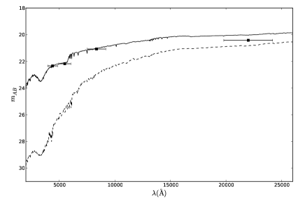
Figure 2: Fit of one LCG (22.0637) photometry with two different galaxy populations. Plain line, the model is fitting the observed photometric points and the dashed line is the model which has passively evolved until z=0. The evolved photometric point are measured by integrating this spectrum.

4 Results and discussion

The velocity dispersion measurements and the stellar mass estimates are listed in the table 2. The velocity dispersions from the absorptions lines of the LCGs range between $\sim 137\ \rm{km/s}$ and $260\ \rm{km/s}$ with a median of $\sim 180\ \rm{km/s}$. The two galaxies with highest velocity dispersion (03.1349 and 03.1540) are ISO galaxies. Hammer (1999) showed that galaxies detected by ISO tend to be large and massive, and found mostly in interacting systems yielding strong star formation rates ($>100\rm{M}_{\odot}\ \rm{yr}^{-1}$).

Table 2: Measurements and results

name	$S/N$	$z$	$M(B)_{AB}$	A(V)	$[O/H]$	$\Delta[O/H]$	$\sigma_{abs}$	$\Delta\sigma_{abs}$	$log(M_{\star})$
			(mag)	(mag)			(km/s)	(km/s)	$(M_{\odot})$
03.0645	12	0.527	-20.45	1.53	8.57	$\pm$0.09	133.3	$\pm$91.2	10.68
03.1349	13	0.616	-21.15	1.08	8.98	$\pm$0.13	196.5	$\pm$15.9	11.14
03.1540	12	0.689	-21.27	3.52	—	—	259.7	$\pm$37.3	10.89
22.0429	12	0.624	-20.02	2.71	8.87	$\pm$0.15	137.0	$\pm$50.0	9.66
22.0637	14	0.542	-20.95	1.20	8.67	$\pm$0.08	183.3	$\pm$10.2	9.95

In Figure 3, we compare stellar masses, $M_{B}$ and $(U-V)$ colour of LCGs with different type of nearby galaxies.

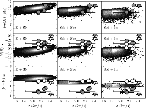
Figure 3: In these figures, the points are the LCGs analyse in this paper, with a triangle for the ISO galaxy not very well fitted by D. Cristobal models. The grey points are the position on the LCGs at the time of the observations and in white the same objects after passive evolution to $z=0$. To find the nature of the LCGs we divided the SDSS data, the reference sample used here, in three different categories: Ellipticals, Spirals and Irregulars galaxies. The crosses represent a local sample of HII galaxies from (Telles & Terlevich, 1997). The upper row is the $M_{\star}$ versus $\sigma$ diagram, the middle one the Faber-Jackson relation $L$ versus $\sigma$ and the lower the colour versus $\sigma$ relation.

The data used for comparison include several different kinds of galaxies taken from the SDSS stellar mass catalogue (Kauffmann et al., 2003). We remark that this catalogue does have some degree of mismatch within a $1\arcsec$ radius with the DR4 catalogue we used for the magnitude and colours. We removed all objects whose cross correlation yielded different plate identification number, different fibre identification number, different modified Julian Date, discrepancies in the redshift or a large error in the measurement of the mass or the velocity dispersion. Our final selection include $\sim$94% of the initial sample.

Figure 3 summarise the results of our analysis. The data points are the 5 LCGs studied in this paper. In grey, the observed value, in white the model predictions after passive evolution. The triangle corresponds to the object whose Stellar Energy Distribution (SED) determined by our stellar mass code did not fit its photometry values. Therefore its estimated evolution is very uncertain. The crosses in the colour-$\sigma$ diagram are HII galaxies (see figure caption). The grey scale are the density plots for different SDSS galaxies. The separation in different galaxies types shown in the three columns was done by colour selection, following Fukugita, Shimasaku, & Ichikawa (1995).

The upper row is the $M_{\star}$ versus $\sigma$ diagram, the middle one the $L$ versus $\sigma$ diagram, and the lower the colour versus $\sigma$ diagram. About $\sim$5 Gyrs ago, the 5 LCGs have stellar masses and velocity dispersions consistent with those characteristic of today’s population of early-type spheroids and spiral galaxies. Their luminosities and colours, however, are similar to most luminous, bluest local HII galaxies. Assuming the stellar masses and velocity dispersions of these LCGs remain approximately constant, and that they are undergoing their last burst of star formation, simple evolutionary synthesis models predict that these objects will evolve passively to best resemble the typical luminosities and colours of early-type spiral galaxies. Our velocity dispersion and stellar mass measurements, combined with this simple evolutionary predictions, are consistent with the proposed link between LCGs and massive spiral galaxies (Hammer et al., 2001).

We note that our results are not necessarily inconsistent with previous works suggesting that other class of intermediate redshift star-forming galaxies (the so-called Luminous Compact Blue Galaxies) may evolve into today’s population of low mass spheroidal galaxies (Koo et al. 2005, Guzmán et al. 2003, Noeske et al. 2006). The LCGs in our sample have a luminosity similar to the 15% brightest objects in the LCBGs samples studied by Koo et al. (2005), and Noeske et al. (2006).

References

- Bender, Burstein, & Faber (1992) Bender R., Burstein D., Faber S. M., 1992, ApJ, 399, 462
- Bruzual A. & Charlot (1993) Bruzual A. G., Charlot S., 1993, ApJ, 405, 538
- Bruzual & Charlot (2003) Bruzual G., Charlot S., 2003, MNRAS, 344, 1000
- Cardiel et al. (1998) Cardiel N., Gorgas J., Cenarro J., Gonzalez J. J., 1998, A&AS, 127, 597
- Calzetti et al. (2000) Calzetti D., Armus L., Bohlin R. C., Kinney A. L., Koornneef J., Storchi-Bergmann T., 2000, ApJ, 533, 682
- Charlot & Longhetti (2001) Charlot S., Longhetti M., 2001, MNRAS, 323, 887
- Conselice, Blackburne, & Papovich (2005) Conselice C. J., Blackburne J. A., Papovich C., 2005, ApJ, 620, 564
- Cristóbal-Hornillos et al. (2005) Cristóbal-Hornillos D., Balcells M., Domínguez-Palmero L., Eliche-Moral C., Erwin P., Guzmán R., Prieto M., 2005, RMxAC, 24, 227
- Cristóbal-Hornillos (2005b) Cristóbal-Hornillos D., 2005, PhDT
- Falcón-Barroso et al. (2011) Falcón-Barroso J., Sánchez-Blázquez P., Vazdekis A., Ricciardelli E., Cardiel N., Cenarro A. J., Gorgas J., Peletier R. F., 2011, A&A, 532, A95
- Fukugita, Shimasaku, & Ichikawa (1995) Fukugita M., Shimasaku K., Ichikawa T., 1995, PASP, 107, 945
- González-González (1993) González-Gonzalez J. D. J., 1993, PhDT
- Gruel (2002) Gruel N., 2002, PhDT
- Guzmán et al. (1997) Guzmán R., Gallego J., Koo D. C., Phillips A. C., Lowenthal J. D., Faber S. M., Illingworth G. D., Vogt N. P., 1997, ApJ, 489, 559
- Guzmán et al. (2003) Guzmán R., Östlin G., Kunth D., Bershady M. A., Koo D. C., Pahre M. A., 2003, ApJ, 586, L45
- Hammer et al. (1995) Hammer F., Crampton D., Le Fevre O., Lilly S. J., 1995, ApJ, 455, 88
- Hammer (1999) Hammer F., 1999, ASPC, 187, 164
- Hammer (2000) Hammer F., 2000, ASPC, 197, 425
- Hammer et al. (2001) Hammer F., Gruel N., Thuan T. X., Flores H., Infante L., 2001, ApJ, 550, 570
- Hempel et al. (2011) Hempel A., Cristóbal-Hornillos, D., Prieto, M., Trujillo, I., Balcells, M., López-Sanjuan, C., Abreu, D., Eliche-Moral, C., Domínguez-Palmero, L., 2011, arXiv, arXiv:1102.3302
- Kauffmann et al. (2003) Kauffmann G., et al., 2003, MNRAS, 341, 33
- Kelson et al. (2000) Kelson D. D., Illingworth G. D., van Dokkum P. G., Franx M., 2000, ApJ, 531, 184
- Kobulnicky & Gebhardt (2000) Kobulnicky H. A., Gebhardt K., 2000, AJ, 119, 1608
- Koo et al. (2005) Koo D. C., et al., 2005, ApJS, 157, 175
- Le Fevre et al. (1995) Le Fevre O., Crampton D., Lilly S. J., Hammer F., Tresse L., 1995, ApJ, 455, 60
- Lehnert & Heckman (1996) Lehnert M. D., Heckman T. M., 1996, ApJ, 472, 546
- Lilly et al. (1995) Lilly S. J., Le Fevre O., Crampton D., Hammer F., Tresse L., 1995, ApJ, 455, 50
- Lilly et al. (1998) Lilly S., et al., 1998, ApJ, 500, 75
- Matković & Guzmán (2005) Matković A., Guzmán R., 2005, MNRAS, 362, 289
- Noeske et al. (2006) Noeske K. G., Koo D. C., Phillips A. C., Willmer C. N. A., Melbourne J., Gil de Paz A., Papaderos P., 2006, ApJ, 640, L143
- Phillips et al. (1997) Phillips A. C., Guzmán R., Gallego J., Koo D. C., Lowenthal J. D., Vogt N. P., Faber S. M., Illingworth G. D., 1997, ApJ, 489, 543
- Pisano et al. (2001) Pisano D. J., Kobulnicky H. A., Guzmán R., Gallego J., Bershady M. A., 2001, AJ, 122, 1194
- Puech et al. (2006) Puech M., Hammer F., Flores H., Östlin G., Marquart T., 2006, A&A, 455, 119
- Salpeter (1955) Salpeter E. E., 1955, ApJ, 121, 161
- Sánchez-Blázquez et al. (2006) Sánchez-Blázquez P., et al., 2006, MNRAS, 371, 703
- Sargent et al. (1977) Sargent W. L. W., Schechter P. L., Boksenberg A., Shortridge K., 1977, ApJ, 212, 326
- Telles & Terlevich (1997) Telles E., Terlevich R., 1997, MNRAS, 286, 183
- Tresse et al. (2002) Tresse L., Maddox S. J., Le Fèvre O., Cuby J.-G., 2002, MNRAS, 337, 369
- Treu et al. (1999) Treu T., Stiavelli M., Casertano S., Møller P., Bertin G., 1999, MNRAS, 308, 1037
- Treu et al. (2001a) Treu T., Stiavelli M., Bertin G., Casertano S., Møller P., 2001, MNRAS, 326, 237
- Treu et al. (2001b) Treu T., Stiavelli M., Møller P., Casertano S., Bertin G., 2001, MNRAS, 326, 221
- Werk, Jangren, & Salzer (2004) Werk J. K., Jangren A., Salzer J. J., 2004, ApJ, 617, 1004
- Zheng et al. (2004) Zheng X. Z., Hammer F., Flores H., Assémat F., Pelat D., 2004, A&A, 421, 847