Mapping the radial structure of AGN tori

We present mid-IR interferometric observations of six type 1 AGNs at multiple baseline lengths ranging from 27 m to 130 m, reaching high angular resolutions up to $\lambda/B\sim 0.02$ arcseconds. For two of the targets, we have simultaneous near-IR interferometric measurements as well, taken within a week. We find that all the objects are partially resolved at long baselines in these IR wavelengths. The multiple-baseline data directly probe the radial distribution of the material on sub-pc scales. We show that for our sample, which is small but spans over $\sim$2.5 orders of magnitudes in the UV/optical luminosity $L$ of the central engine, the radial distribution clearly and systematically changes with luminosity.

The brightness distribution at a given mid-IR wavelength seems to be rather well described by a power law, which makes a simple Gaussian or ring size estimation quite inadequate. In this case, a half-light radius $R_{\rm 1/2}$ can be used as a representative size. We show that the higher luminosity objects become more compact in normalized half-light radii $R_{\rm 1/2}/R_{\rm in}$ in the mid-IR, where $R_{\rm in}$ is the dust sublimation radius empirically given by the $L^{1/2}$ fit of the near-IR reverberation radii. This means that, contrary to previous studies, the physical mid-IR emission size (e.g. in pc) is not proportional to $L^{1/2}$, but increases with $L$ much more slowly. With our current datasets, we find that $R_{\rm 1/2}\propto L^{0.21\pm 0.05}$ at 8.5 $\mu$m, and $R_{\rm 1/2}$ nearly constant at 13 $\mu$m.

The derived size information also seems to correlate with the properties of the total flux spectrum, in particular the smaller $R_{\rm 1/2}/R_{\rm in}$ objects having bluer mid-IR spectral shape. We use a power-law temperature/density gradient model as a reference, and infer that the radial surface density distribution of the heated dust grains at a radius $r$ changes from a steep $\sim$$r^{-1}$ structure in high luminosity objects to a shallower $\sim$$r^{0}$ structure in those of lower luminosity. The inward dust temperature distribution does not seem to smoothly reach the sublimation temperature – on the innermost scale of $\sim$$R_{\rm in}$, a relatively low temperature core seems to co-exist with a slightly distinct brightness concentration emitting roughly at the sublimation temperature.

1 Introduction

A key step in understanding the accretion process in active galactic nuclei (AGN) is to determine the role and structure of the putative obscuring torus. The obscuration here essentially refers to the radiative absorption by dust grains in the torus, which hides the UV/optical emission of the central engine and the broad line emission (see Antonucci 1993 for a review). In type 2 objects, which do not display these spectral components, our line of sight towards the nucleus is thought to be relatively close to the system’s equatorial direction along which the torus obscuration becomes effective. Type 1 objects are believed to be rather face-on and permit us to directly observe the central components unobscured. The torus dust grains thermally re-emit the absorbed energy, and the innermost dust sublimates at $\sim$1500 K, setting the inner boundary of the dust distribution. This dust sublimation region thus radiates mostly in the near-infrared (near-IR; wavelength $\lambda$ $\sim$ a few $\mu$m), with outer dust grains emitting at lower temperatures in the mid-IR ($\sim$10 $\mu$m). Without much spatial information, the torus structure has long been inferred from the observed spectral energy distributions (SEDs) mainly in the near- and mid-IR, as well as theoretical arguments.

The SEDs were first modeled by the tori with smooth density distributions (Pier & Krolik 1993; Granato & Danese 1994; Efstathiou & Rowan-Robinson 1995). However, the case for the material being in a clumpy medium has theoretically been argued from an early stage (Krolik & Begelman 1988). Accordingly, there have been many efforts to develop clumpy torus models in the past decade (Nenkova et al. 2002; Dullemond & van Bemmel 2005; Hönig et al. 2006; Schartmann et al. 2008; Nenkova et al. 2008a; Hönig & Kishimoto 2010), and the torus structure has been inferred in the context of these clumpy torus models (Nenkova et al. 2008b; Ramos Almeida et al. 2009; Mor et al. 2009; Hönig et al. 2010; Ramos Almeida et al. 2011; Alonso-Herrero et al. 2011). However, we are finally beginning to have far more direct information with the long-baseline interferometry in both the near- and mid-IR by spatially resolving the inner structure.

1.1 Early Type 2 investigations

Detailed interferometric studies in the mid-IR have targeted a few bright type 2 AGNs, with the first ones being NGC1068 and Circinus (Jaffe et al. 2004; Tristram et al. 2007), using the mid-infrared interferometric instrument (MIDI) at the Very Large Telescope Interferometer (VLTI). These have achieved the first determination of the overall size and projected orientation of the mid-IR emission region with two-temperature elliptical Gaussian models. The AGN NGC1068 was also successfully observed with the near-IR (2.2 $\mu$m) long-baseline interferometric instrument VINCI at VLTI (Wittkowski et al. 2004), and followed up in the mid-IR with more detailed MIDI observations (Raban et al. 2009). One hard aspect is that, since the nucleus is heavily obscured in type 2 objects, one needs to disentangle the effects of radiative transfer in order to study the intrinsic structure and distribution of the material. Another type 2 object, Cen A, was the first radio-loud object to be studied with the IR long-baseline interferometry (Meisenheimer et al. 2007), which was followed by more detailed observations by Burtscher et al. (2010). Interestingly, the corresponding mid-IR source is found to be dominated by an unresolved source, interpreted to be a synchrotron core, which might, however, also complicate the study of the structure.

1.2 Type 1 study in the near-IR

Studies of type 1 objects are largely unaffected by the inclination/obscuration. We can directly scrutinize the inner intrinsic structure in both the near-IR and mid-IR. In the near-IR, Swain et al. (2003) made the first measurement of the K-band (2.2 $\mu$m) visibility of the brightest type 1 AGN NGC4151 with the Keck interferometer (KI), where they obtained quite high visibility (squared visibility $V^{2}\sim 0.8$). This result was recently confirmed by Kishimoto et al. (2009a) and also Pott et al. (2010). Furthermore, Kishimoto et al. (2009a, 2011) found similarly high visibilities for in total eight type 1 AGNs. They argued that this is an indication of the marginal and partial resolution of the dust sublimation region in these type 1 AGNs. Firstly, they marginally detected a visibility decrease over the baseline length for NGC4151, which would be robust evidence for a partially resolved structure. Secondly, its implied size calculated as a geometric thin-ring radius for NGC4151 as well as those for the other type 1s are found to roughly match independent radius measurements from near-IR reverberations, which are thought to be probing the dust sublimation radius.

The near-IR reverberation radius $R_{\rm\tau_{K}}$ is the light-crossing distance over the time lag between the variabilities in the UV/optical and near-IR (2.2 $\mu$m). The former emission is thought to originate from the central accretion disk (AD) and the latter from the hot dust grains in the sublimation region heated by the AD (e.g. Glass 2004; Minezaki et al. 2004; Suganuma et al. 2006; Koshida et al. 2009). The radius $R_{\rm\tau_{K}}$ has been shown to be proportional to $L^{1/2}$ where $L$ is the AGN luminosity (Suganuma et al. 2006; our specific definition of $L$ is given in Sect.3.1), thus, the interferometric ring radii at K-band described above also roughly scale with $L^{1/2}$. This is what we would expect for the dust sublimation radii (e.g. Barvainis 1987). In addtion, the measured ring radii have been shown to be almost unaffected by the near-IR AD component (Kishimoto et al. 2007, 2009a). Therefore, the case for the near-IR visibilities probing the dust sublimation region is strongly made.

Furthermore, Kishimoto et al. (2009a, 2011) pointed out that the ring radii derived from the observed visibilities are either roughly equal to or slightly larger than the $L^{1/2}$-fit to the reverberation radii as a function of $L$. Since reverberation measurements generally place weight on the small responding radii (e.g. Koratkar & Gaskell 1991), $R_{\rm\tau_{K}}$ is expected to represent the radius very close to the inner boundary of the dust distribution. On the other hand, the interferometric ring radii rather correspond to brightness-weighted effective radii. In this sense, the $L^{1/2}$-fit reverberation radius gives a good normalization for the radial extent, taking out the simple $L^{1/2}$ scaling. This normalization is used extensively in this paper.

1.3 Type 1 study in the mid-IR

In the mid-IR, Beckert et al. (2008) presented the first long-baseline mid-IR interferometry for a type 1 AGN, NGC3783. Kishimoto et al. (2009b) published two-baseline data for the same galaxy, revising the results shown in Beckert et al. (2008) with dedicated software (see more details below) and also adding one more data set taken at a different baseline. They proposed a generic way of implementing a uniform comparison of the interferometric data from different targets with different luminosities and at different distances, by using the inner radius $R_{\rm in}$ described above for normalizing the spatial scale probed by the inteferometer. Mainly using the data of NGC3783, but supplementing them with those from other type 1s and the type 2 AGN NGC1068, they argued that the radial brightness distribution in the mid-IR of type 1 AGNs seems to follow a relatively shallow power-law. This was a first attempt to directly map the radial distribution in type 1 AGN tori.

Subsequently, Burtscher et al. (2009) also presented two-baseline MIDI data for another type 1 AGN, NGC4151, and measured the mid-IR emitting region size using a model of a Gaussian plus point-source, which gives a visibility curve relatively similar to that of a power-law at low spatial frequencies. Tristram et al. (2009) presented the results of a MIDI snap-shot survey for AGNs of both types 1 and 2, and discussed the mid-IR emission size as a function of luminosity, which has recently be further evaluated with additional data by Tristram & Schartmann (2011).

Here we present a first systematic investigation of type 1 AGNs with the mid-IR interferometer, expanding the study of Kishimoto et al. (2009b). Combining our mid-IR data with the near-IR interferometry and photometry, we aim to comprehensively map the radial structure of the thermally emitting dusty region in the mid- and near-IR. We aim to derive physical constraints as directly as possible from the observations, with the ultimate goal of finding whether the radial structure is systematically dependent on the properties of the central engine.

Table 1: Properties of our targets and their point-source flux from our UKIRT images or 2MASS images.

name	$z^{a}$	scaleb	$E_{B-V}^{c}$	date	flux (mJy)d					$A_{V}$	$R_{\rm\tau_{K}}$ fite ($\equiv$ $R_{\rm in}$)		$\nu L_{\nu}(5500\AA)^{f}$
	corr.	(pc/mas)	(mag)	(UT)	Z	Y	J	H	K	(mag)	(pc)	(mas)	(erg s-1)b
NGC4151	0.00414	0.0855	0.028	2009-06-17	39.7	42.4	59.4	96.3	173.		0.033	0.383	$(8.3\pm 1.3)\cdot 10^{42}$
NGC3783g	0.0108	0.221	0.119	1999-04-11	—	—	19.1	33.5	62.5		0.061	0.274	$(2.8\pm 0.4)\cdot 10^{43}$
ESO323-G77g	0.0159	0.324	0.101	1999-05-03	—	—	28.6	63.4	107.	1.2$\pm$0.4	0.10	0.321	$(8.4\pm 1.9)\cdot 10^{43}$
H0557-385	0.0342	0.681	0.043	2009-12-13	4.03	4.43	7.21	15.3	36.8	1.5$\pm$0.5	0.12	0.181	$(1.2\pm 0.3)\cdot 10^{44}$
IRAS09149g,h	0.0579	1.12	0.182	2000-01-05	—	—	35.3	59.1	116.		0.47	0.419	$(1.7\pm 0.2)\cdot 10^{45}$
IRAS13349i	0.108	1.98	0.012	2009-06-17	7.75	8.71	12.6	26.3	62.3	0.93$\pm$0.31	0.49	0.248	$(1.9\pm 0.4)\cdot 10^{45}$

^a CMB corrected value from NED. ^b $H_{0}=70$ km s^-1 Mpc^-1, $\Omega_{\rm m}=0.3$, and $\Omega_{\Lambda}=0.7$. ^c Galactic reddening from Schlegel et al. (1998). ^d Flux measurement uncertainty is $\sim$5 % (see Sect.3 in Kishimoto et al. 2009a). ^e The K-band reverberation radius $R_{\rm\tau_{K}}$ from UV luminosity using the fit by Suganuma et al. (2006), which is defined as $R_{\rm in}$ in this paper (see Eq.1). ^f Optical luminosity at rest wavelength 5500Å. ^g From 2MASS images. ^h IRAS09149-6206. ⁱ IRAS13349+2438.

Table 2: MIDI observation log

date & time		telescope	$B_{p}$	PA	vis./flux	max
(UT)			(m)	($\degr$)	calibrator	S/Na
NGC4151
2009-05-09	01:20	UT1-UT3	61.5	55.9	HD94264	4.1
2009-05-09	01:32	UT1-UT3	64.1	55.7	HD94264	3.3
2009-05-09	02:37	UT1-UT3	77.3	53.0	HD98262	3.3
2009-05-09	02:49	UT1-UT3	79.3	52.3	HD98262	3.4
2009-05-10	00:44	UT1-UT2	26.7	45.1	HD94264	5.1
2009-05-10	00:55	UT1-UT2	28.1	46.1	HD94264	4.9
2009-05-11	00:33	UT1-UT4	102.0	84.8	HD113996	4.1
2009-05-11	00:44	UT1-UT4	105.1	83.1	HD113996	4.3
2009-05-11	01:19	UT1-UT4	113.4	78.3	HD94264	4.2
2009-05-11	01:31	UT1-UT4	115.8	76.7	HD94264	4.0
2009-05-12	01:59	UT1-UT4	121.3	72.4	HD94264	3.6
2009-05-12	02:28	UT1-UT4	125.2	68.3	HD98262	3.3
NGC3783
2005-05-28	03:39	UT1-UT2	44.4	45.1	HD100407	3.1
2005-05-28	04:00	UT1-UT2	42.6	45.9	HD100407	5.6
2005-05-31	03:01	UT2-UT4	68.7	114.8	HD100407	3.2
2005-05-31	03:21	UT2-UT4	64.9	119.6	HD100407	3.7
2009-05-11	03:31	UT1-UT4	108.3	80.4	HD112213	3.7
2009-05-11	23:19	UT1-UT4	128.4	45.0	HD101666	4.5
2009-05-11	23:33	UT1-UT4	129.0	47.3	HD101666	4.2
ESO323-G77
2009-05-08	01:01	UT3-UT4	56.8	94.4	HD112213	2.1b
2009-05-08	01:06	UT3-UT4	57.3	95.3	HD112213	2.5b
2009-05-10	03:06	UT1-UT2	54.1	30.5	HD112213	3.8
2009-05-10	03:18	UT1-UT2	53.8	31.8	HD112213	3.4
2009-05-10	04:09	UT1-UT2	51.8	37.1	HD112213	3.8
2009-05-10	04:21	UT1-UT2	51.3	38.1	HD112213	4.1
2009-05-11	04:07	UT1-UT4	118.4	75.0	HD112213	4.2
2009-05-12	00:05	UT1-UT4	126.9	36.9	HD112213	3.9
2009-05-12	00:16	UT1-UT4	127.6	39.1	HD112213	3.6
H0557-385
2009-05-09	23:33	UT1-UT2	42.1	46.4	HD40808	3.6
2009-05-09	23:45	UT1-UT2	41.0	46.8	HD40808	4.0
2009-08-02	09:14	UT3-UT4	32.9	60.3	HD9362	3.8
2009-08-03	09:02	UT1-UT2	56.3	-12.9	HD39425	3.7
2009-08-05	09:48	UT1-UT4	120.0	17.4	HD40808	3.5
IRAS09149-6206
2009-03-15	00:29	UT1-UT2	49.9	13.0	HD80007	3.9
2009-03-15	00:39	UT1-UT2	49.7	14.7	HD80007	3.8
2009-05-08	00:25	UT3-UT4	62.4	126.4	HD89682	2.3b
2009-05-08	01:45	UT3-UT4	62.4	144.2	HD89682	2.5b
2009-05-08	02:01	UT3-UT4	62.3	148.0	HD89682	2.0b
2009-05-09	00:18	UT1-UT3	80.2	53.4	HD89682	3.6
2009-05-09	00:30	UT1-UT3	78.9	55.4	HD89682	4.2
2009-05-10	23:38	UT1-UT4	119.2	77.4	HD89682	4.2
2009-05-10	23:49	UT1-UT4	118.0	79.8	HD89682	4.6
IRAS13349+2438
2009-05-10	01:51	UT1-UT2	34.7	28.6	HD113996	3.2
2009-05-10	02:30	UT1-UT2	38.2	33.6	HD113996	3.2
2009-05-10	04:40	UT1-UT2	49.3	39.3	HD112213	4.6
2009-05-11	02:40	UT1-UT4	116.2	71.1	HD113996	4.5
2009-05-11	02:51	UT1-UT4	118.7	70.3	HD113996	4.9
2009-05-12	01:06	UT1-UT4	89.9	76.2	HD113996	3.5
2009-05-12	01:18	UT1-UT4	93.9	75.6	HD113996	3.3
2009-05-12	04:11	UT1-UT4	129.3	63.7	HD127093	5.1

^a Maximum signal-to-noise ratio (SNR) per smoothed frame for the correlated
flux integraged over the whole N-band (see Appendix for details).
^b Excluded from the analyses in this paper due to low SNR.

2 Observations and data reductions

2.1 MIDI

We observed six type 1 AGNs listed in Table 1 on 8-12 May 2009 (UT) using MIDI, which is a two-beam combiner working in the mid-IR wavelengths (Leinert et al. 2003). The observation log for each fringe track is listed in Table 2. We also collected a limited number of data sets for two of the six targets on 15 Mar and 5 Aug 2009 (Table 2). The adaptive optics system MACAO at each of the 8.2m Unit Telescopes was locked on the nucleus of each target AGN. A single baseline was allocated for each night, and we used four different baselines with their projected length spanning from 27 m to 129 m. For one of the targets, NGC3783, we also used in our analysis MIDI data taken in 2005 published by Beckert et al. (2008) and Kishimoto et al. (2009b).

The data were reduced using the software EWS (version 1.7.1; Jaffe 2004), but with modifications using our own IDL codes. The old NGC3783 data were also re-reduced with the same procedure. The details of the process are described in the Appendix A. Briefly, we firstly implemented an additional background subtraction for the photometry frames using adjacent sky strips in the 2D spectrum. Secondly, to reduce errors in group delay determinations, we smoothed delay tracks over typically $\sim$20-40 frames. To avoid possible positive biases in the correlated flux, we also averaged $\sim$20-40 frames to determine the phase offsets. The system visibility was obtained from the observations of visibility calibrators taken right after or before each target observation with a similar airmass. These data were also reduced with similar smoothings above to calibrate out the effect of the time averaging. These calibrators are also the photometric standards found in the list by Cohen et al. (1999) and/or by R. van Boekel (priv. communication). We obtained the correlated flux, which was corrected for the system visibility, and total flux separately. The errors for the total flux and correlated flux were firstly estimated from the fluctuation of the measurements over time. The total flux spectrum for each object was then derived as the weighted mean of many measurements over different nights (for NGC3783, the spectrum was derived separately for 2005 and 2009 data; see below). For the correlated flux measurements at adjacent $uv$ points, we also took weighted means. Finally, for the correlated flux, we assigned a systematic uncertainty as a 5% of the total flux based on the analysis presented in Appendix A.

For NGC3783, the mid-IR total flux apparently increased by $\sim$20% from 2005 to 2009 observations. To facilitate a direct comparison, we scaled the total flux and correlated flux from the 2005 observations by the same factor. This means that we assumed no visibility change in the mid-IR over this period. This is conceivable based on a comparison of near-IR interferometry data for NGC4151 that found no significant visibility change over a one-year timescale (Pott et al. 2010; Kishimoto et al. 2011).

To test the accuracy of our MIDI reduction software specifically for targets at sub-Jy flux levels, we observed stars with flux $\sim$0.3–0.8 Jy at 12 $\mu$m during our May 2009 run, and also in Mar 2009. Details are described in Appendix A. One significant issue is that, if the frames are not averaged over a sufficiently long time-interval, the correlated flux is affected by a positive bias apparently in the wavelength region for which there are lower (intrinsic) counts. Since MIDI count spectra often have a peak at shorter wavelengths, the resulting biased spectrum is often redder than it should be. In addition, coherence loss toward shorter wavelengths might not be fully compensated for by calibrator frames, leading also to redder correlated-flux spectra. With the data for the sub-Jy unresolved stars, we demonstrate that the dedicated codes can correctly estimate the correlated flux, and quantify the possible systematic uncertainty.

In Table 2, the quality of each fringe track is indicated by the maximum signal-to-noise ratio (S/N) per smoothed frame (see Sect.A.3). The analysis of the sub-Jy unresolved stars described above currently covers this S/N down to $\sim$2.5, thus in this paper we decided not to use data with a S/N lower than 2.5. Accordingly, five fringe tracks in Table 2 were excluded from our analysis.

2.2 The near-IR data

We combined the mid-IR MIDI data above with data in the near-IR to comprehensively map the radial structure of the thermally emitting dusty region. For the photometry in the near-IR, we have contemporaneous imaging data at five broad-band wavelengths from 0.9 to 2.2 $\mu$m for NGC4151, IRAS13349, and H0557-385, taken with the Wide Field Camera (WFCAM) on the United Kingdom Infrared Telecope (UKIRT). The data for the former two objects were published in Kishimoto et al. (2009a), but, together with the new data for H0557-385, we present here the data for all three AGNs in Table 1. The wide field-of-view of WFCAM provides simultaneous point-spread-function (PSF) measurements from stars in the same field. We used them to implement accurate PSF + host galaxy fits, and measured the point-source-only SEDs in the near-IR (see Kishimoto et al. 2009a for more details). For the three other targets in the sample, we measured the point-source flux by applying the same procedure to 2MASS images.

We have the near-IR interferometry data taken with the Keck interferometer (KI) at 2.2 $\mu$m for two of the six MIDI targets, NGC4151 and IRAS13349. The KI data were taken on 15 May 2009 (Kishimoto et al. 2009a), less than a week from our MIDI observations of these targets. For the general comparison over the sample between the mid- and near-IR, we also use the sample of in total eight type 1 AGNs, taken with the KI in the near-IR at 2.2 $\mu$m (Kishimoto et al. 2009a, 2011).

2.3 VISIR

To obtain accurate photometry and check the accuracy of the total flux spectra from MIDI, we took mid-IR images of each object in two passbands, namely at 8.6 $\mu$m and 11.9 $\mu$m with VISIR on UT3. These images were mostly taken within about four weeks of the MIDI observations, to minimize the effect of variability. The observation log and the results are shown in Table 3. For ESO323-G77, a VISIR spectrum was taken by Hönig et al. (2010) within several days of our MIDI observations.

All the VISIR images were taken in ’perpendicular’ mode with each dataset consisting of four image tiles. Using the data from the ESO pipeline (version 3.7.2), we implemented additional subtraction of the background determined at annuli of radii $\sim 1.5-3.0^{\prime\prime}$ from each source on each of the four tiles. After checking the stability of the flux calibration as a function of aperture radii, we determined the flux conversion factor at a radius $\sim$$1^{\prime\prime}$ where its uncertainty was estimated from the scatter in the results from the four tiles.

2.4 Additional photometric data in the mid-IR and near-IR

When fitting the models described in the next section to the SEDs, we only used our MIDI total flux spectra and WFCAM (or 2MASS) point-source fluxes described above. However, we gathered in addition IRS spectra and IRAC imaging data from the Spitzer Heritage Archive, listed in Table 4, for all the targets. For NGC3783, we also have VLT/ISAAC data taken on 2 Jan 2011 (Hönig et al. in prep; Table 4). These extra data points from Spitzer and ISAAC fall approximately on our model SEDs presented below, with possibly some additional flux from the host galaxy, thus are viewed as approximate upper limits, and not used in the spectral fitting. We summarize the usage of our data in Table 5.

Table 3: The results of our VISIR imaging observations.

name	flux	aperturea	UT date	calibrator
	(mJy)	(arcsec)
PAH1 at $\lambda$ 8.59 $\mu$m, $\Delta\lambda$ 0.42 $\mu$m
NGC4151	860$\pm$17	1.8	2009-06-07	HD120933
NGC3783	423$\pm$24	1.5	2009-06-07	HD145897
H0557-385	330$\pm$18	1.5	2009-09-07	HD41047
IRAS09149	346$\pm$10	1.5	2009-06-07	HD99167
IRAS13349	389$\pm$10	1.5	2009-06-07	HD145897
PAH2ref2 at $\lambda$ 11.88 $\mu$m, $\Delta\lambda$ 0.37 $\mu$m
NGC4151	1432$\pm$53	2.7	2009-06-07	HD120933
NGC3783	760$\pm$17	1.5	2009-06-07	HD145897
H0557-385	404$\pm$29	1.5	2009-09-07	HD41047
IRAS09149	474$\pm$31	1.5	2009-06-07	HD99167
IRAS13349	530$\pm$26	1.5	2009-06-08	HD145897

^a Aperture diameter for target and calibrator for flux determination.

Table 4: Spizer data from Spitzer Heritage Archive and ISAAC/VLT data.

name	IRS	IRAC flux (mJy)
	date (UT)	date (UT)	3.6 $\mu$m	4.5 $\mu$m	5.7 $\mu$m	7.9 $\mu$m
NGC4151	2004-01-08	2004-12-17	264.9$\pm$1.0	363.8$\pm$1.2	554.0$\pm$3.2	924.7$\pm$2.3
NGC3783	2007-06-27	2007-08-07	118.0$\pm$0.7	158.5$\pm$0.8	228.1$\pm$2.3	359.6$\pm$1.5
ESO323-G77	2006-08-05	2009-03-14	185.6$\pm$0.8	215.4$\pm$1.0	288.3$\pm$2.4	411.2$\pm$1.6
H0557-385	2007-10-06	2008-10-31	140.7$\pm$0.7	195.3$\pm$0.9	268.8$\pm$2.4	344.0$\pm$1.5
IRAS09149	2008-07-02	2008-05-13	214.4$\pm$0.9	261.9$\pm$1.1	330.9$\pm$2.6	391.8$\pm$1.6
IRAS13349	2005-06-07	2009-02-02	199.1$\pm$4.2	242.6$\pm$1.0	300.1$\pm$4.2	431.4$\pm$1.7
name	ISAAC flux (mJy)
	date (UT)	2.25 $\mu$m	3.80 $\mu$m	4.66 $\mu$m
NGC3783	2011-01-02	66.21$\pm$0.61	107.00$\pm$0.49	152.83$\pm$4.65

Table 5: Summary of the data used for each target.

name	data used for modeling				additional photometric data only for		polar-
	near-IR		mid-IR		confirmation or approximate upper limits		axisa
	1-2.2 $\mu$m flux	interferometry	total flux	interferometry	3-15 $\mu$m	mid-IR	PA(°)
NGC4151	WFCAM/UKIRT	Keck	MIDI spectrum	MIDI	IRAC / IRS	VISIR images	91b
NGC3783	2MASS	–	MIDI spectrum	MIDI	ISAAC / IRAC / IRS	VISIR images	136c
ESO323-G77	2MASS	–	MIDI spectrum	MIDI	IRAC / IRS	VISIR spectrum	174d
H0557-385	WFCAM/UKIRT	–	MIDI spectrum	MIDI	IRAC / IRS	VISIR images	33e
IRAS09149	2MASS	–	MIDI spectrum	MIDI	IRAC / IRS	VISIR images	–
IRAS13349	WFCAM/UKIRT	Keck	MIDI spectrum	MIDI	IRAC / IRS	VISIR images	35f

^aThe PA of the polar axis of the system inferred from optical polarization and radio axis.
^bMartel (1998); Mundell et al. (2003). ^cSmith et al. (2002). ^dSchmid et al. (2003). ^eBrindle et al. (1990). ^fWills et al. (1992).

2.5 Reddening corrections

We corrected the SED for Galactic reddening using values from Schlegel et al. (1998) listed in Table 1. We used the reddening curves of Cardelli et al. (1989), supplemented with that of Chiar & Tielens (2006) at long wavelengths. We also corrected the SED for the possible reddening within the host galaxy for IRAS13349, ESO323-G77, and H0557-385, using the $A_{V}$ values listed in Table 1. For H0557-385, in terms of the optical continuum slope, Balmer decrement, and host galaxy inclination (Winkler 1992; Fairall et al. 1982), the reddening is likely to be between those of ESO323-G77 and IC4329A, which is another Seyfert 1 galaxy known to be strongly affected by host reddening. For the latter two objects, the estimates of $A_{V}$ from the different methods exist including that derived from the gradients of flux variation (Winkler et al. 1992), and are $\sim$1 and $\sim$2, respectively (Winkler et al. 1992). Without any additional solid information about the reddening value for H0557-385, we roughly infer that $A_{V}=1.5\pm 0.5$.

3 Results

3.1 The whole data sets and prerequisites

Figures 1 and 2 present all the data for each of the six targets. The total and correlated flux spectra are shown in the top panel, the visibility as a function of spatial frequency in the middle, and the $uv$ coverage in the bottom. In the top panel, all the additional flux data described in the previous section are also plotted. The MIDI data were binned by seven pixels ($\Delta\lambda\sim 0.4\mu$m) with the error in each bin taken as the median of the errors over the binned spectral channels (since errors over adjacent channels are correlated).

For the visibilities, the spatial frequency is shown in units of cycles per $R_{\rm in}$. As described in Sect. 1.2, as the most empirical measure of the inner radius $R_{\rm in}$ of the dust distribution, we adopt the $L^{1/2}$ fit to the K-band reverberation radius $R_{\rm\tau_{K}}$ given by Suganuma et al. (2006). Here $L$ is the UV luminosity of the central engine, which is defined as a scaled optical luminosity, $L=6\nu L_{\nu}(5500\AA)$ (Kishimoto et al. 2007), assuming a generic SED over the UV/optical wavelengths. Here $\nu$ designates the frequency in the rest frame, and $L_{\nu}$ is the isotropic luminosity per frequency. The formula for the $L^{1/2}$ fit by Suganuma et al. (2006) is given in Kishimoto et al. (2007) as

$$R_{\rm in}\equiv R_{\rm\tau_{K}}=0.47\cdot\left(\frac{6\nu L_{\nu}(5500\AA)}{10^{46}\ {\rm erg/sec}}\right)^{1/2}\ {\rm pc}.$$ (1)

If the dust temperature structure is primarily determined by the illumination from the central source, the radial temperature structure scales with the sublimation radius $R_{\rm in}$. In this case, by normalizing a length scale with $R_{\rm in}$, we can place various interferometric data on a uniform scale (Kishimoto et al. 2009b). A given configuration of an interferometer probes a certain spatial frequency, or a certain spatial scale represented by a spatial wavelength, which is the reciprocal of the spatial frequency. Here we normalize this spatial wavelength with $R_{\rm in}$ (see the upper axis of the middle panel of Figs.1 and 2). This corresponds to writing the spatial frequency in units of cycles per $R_{\rm in}$. With this normalization, we can eliminate the simple luminosity scaling originating from $R_{\rm in}$ being proportional to $L^{1/2}$, as well as a simple distance scaling. Different objects with different luminosities and at various distances have different angular sizes for $R_{\rm in}$, but the data can be uniformly viewed when the probed spatial scale is normalized with $R_{\rm in}$. We can further directly determine whether there is a luminosity dependence in the structure beyond the simple $L^{1/2}$ scaling.

Following the same idea, the total and correlated fluxes can be normalized using $R_{\rm in}^{2}$. They are shown in the top panel of Figs.1 and 2 as $(\nu L_{\nu}/4\pi)/R_{\rm in}^{2}$ and have the same dimension as the surface brightness in the rest frame of each target. This is equal to $\nu_{\rm obs}f_{\nu_{\rm obs}}\cdot(1+z)^{4}/\theta_{\rm in}^{2}$, where $\nu_{\rm obs}$, $f_{\nu_{\rm obs}}$, and $\theta_{\rm in}$ are the frequency, observed flux, and angular size of $R_{\rm in}$ in the observed frame, respectively. The correlated flux in the top panel is color-coded with the spatial wavelength, while each visibility data point in the middle panel is color-coded with the (radiation) wavelength in the rest frame, as indicated by the color bars. The total flux, correlated flux, and visibility spectra are shown in Appendix B using more conventional units to facilitate direct comparisons with the data in the literature.

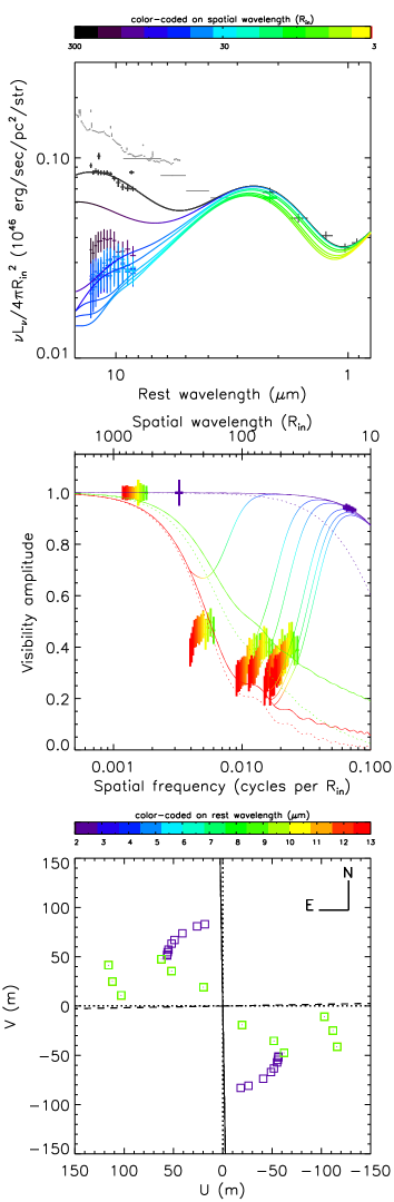
(a) NGC4151

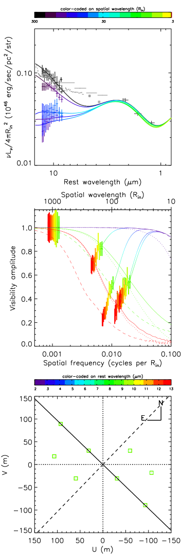
(b) NGC3783

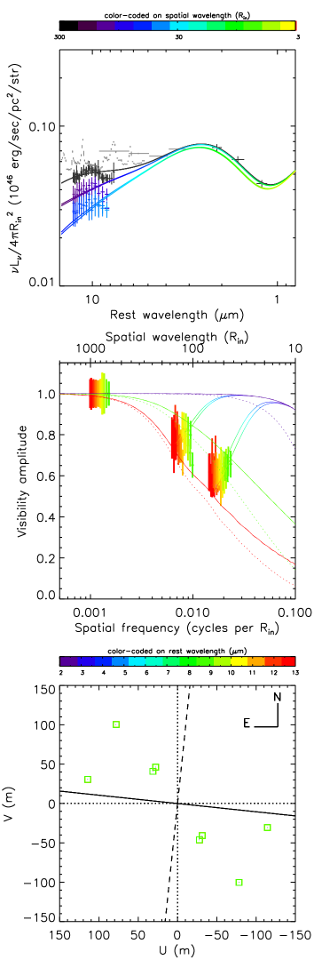
(c) ESO323-G77

Figure 1: The observed data for (a) NGC4151, (b) NGC3783, and (c) ESO323-G77 (see Sect.2), and the best fits using a temperature/density gradient model plus an inner 1400K ring (see Sect.4.4 and Table 8). Top: Spectral energy distribution in $(\nu L_{\nu}/4\pi)/R_{\rm in}^{2}$. The data plotted in black are the total flux measurements from MIDI and VISIR in the mid-IR and from WFCAM or 2MASS in the near-IR. Additional total flux spectra and photometry from Spitzer (Table 4) are plotted in gray. For NGC3783, ISAAC photometry data (Table 4) are shown as gray squares. Correlated fluxes from the mid-IR and near-IR interferometry are plotted with colors coded on spatial wavelengths in units of $R_{\rm in}$ as shown in the top color bar. The model curves for the total flux and the correlated fluxes at baselines corresponding to each MIDI observation are drawn in the same color coding. Middle: Visibility amplitude plotted against spatial frequency in units of cycles per $R_{\rm in}$. The color of the data points corresponds to the observing wavelength in the rest frame of the target. This color-coding is shown as a color bar between the middle and bottom panels. The iso-wavelength model visibility curves are shown for 13, 8.5, and 2.2$\mu$m, as well as the curves for each baseline configuration (which are ’orthogonal’ to the iso-wavelengh curves). Dotted curves are the visibilities only for the power-law component, with the difference from solid curves indicating the effect of the near-IR ring. For NGC3783, solid and dashed model curves are for equatorial and polar axis PAs, respectively (see Sect.4.3). Bottom: The $uv$ coverage of the mid-IR and near-IR interferometry with the same color-coding on observing wavelengths. Solid and dashed lines indicate the PA of the projected equatorial and polar axes, respectively, inferred from optical polarization and radio data (see Table 5).

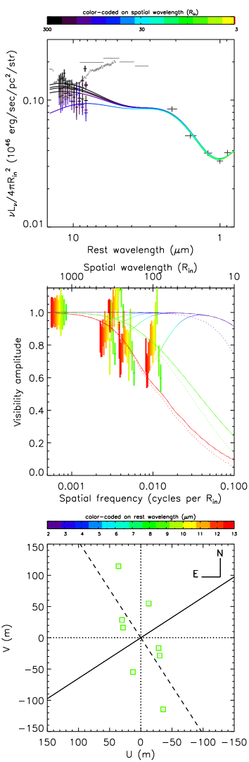
(a) H0557-385

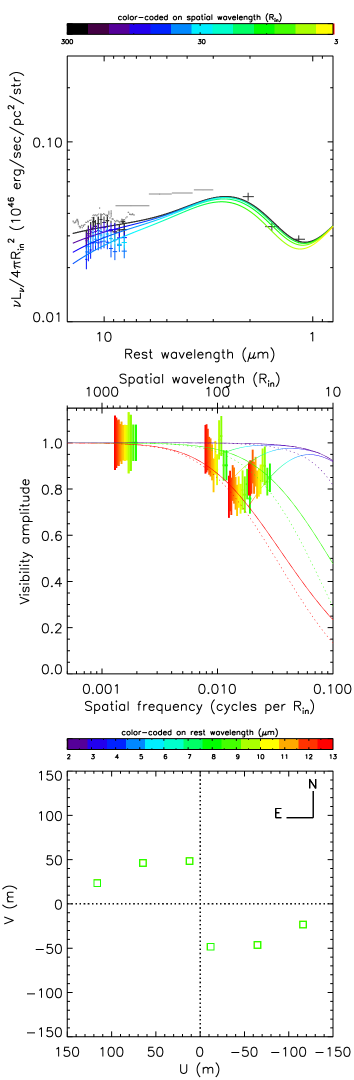
(b) IRAS09149

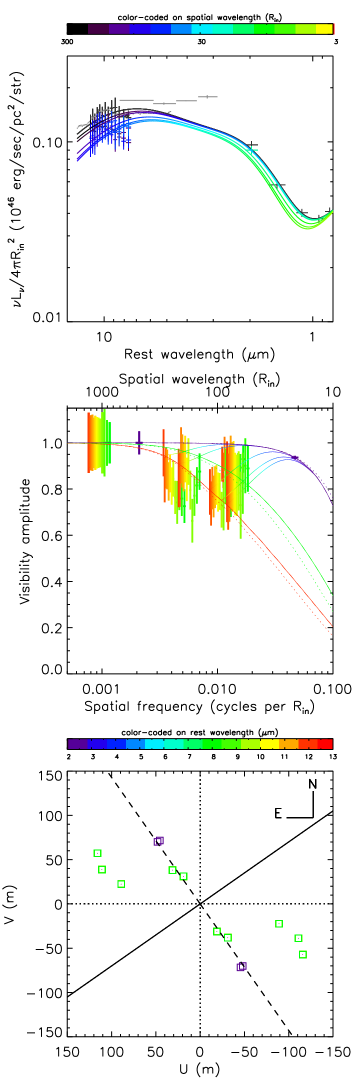
(c) IRAS13349

Figure 2: The same as Fig.1, but for (a) H0557-385 (b) IRAS09149 (c) IRAS13349.

3.2 MIDI total flux spectra

With MIDI, total fluxes are measured separately and independently of correlated flux measurements. We derived a total flux spectrum for each object as a weighted mean of many measurements over different nights. The fluxes from our VISIR photometry (or VISIR spectrum in the case of ESO323-G77) were found to be either in excellent agreement (within a few percent) with or slightly larger ($\sim$10$-$20%; see Appendix B) than the mean MIDI total flux spectrum for each object. Since the latter is from the beams corrected with MACAO and from a smaller extraction window (adaptive mask in EWS), it is conceivable that it has less contribution from the extended emission, e.g. from the host galaxy. In the case of NGC4151, which seems to have quite an extended mid-IR emission (see the low visibilities in Fig.1a), some of the extended emission in the VISIR flux is probably excluded in the MIDI flux. All these comparisons with VISIR fluxes confirm the accuracy of the mean MIDI total flux, and its error might be slightly over-estimated in some cases.

In the middle panel for visibilities in Figs.1 and 2 (and also in Fig.3 discussed in the next section), we show the visibility uncertainties originating from each correlated flux measurement without the contribution of total flux errors, but show the total flux errors separately as data points of visibility unity at the lowest spatial frequency. In this way, we can clearly show the relative uncertainties between each correlated flux measurement and the total flux measurement. In addition, these total flux data points are shown at the spatial frequency with the baseline length equal to the single telescope diameter. As long as the source remains unresolved by a single telescope, the total flux gives the correlated flux at this spatial frequency, and the visibility is unity at this spatial frequency. Thus, the data points illustrate the constraint in such a case, which is expected to hold at least approximately for our sample of type 1 objects. We note however that these are only for the data presentation. For the model fitting in Sect.3.5 and 4, we include the total flux error in the visibility error budget in a normal way.

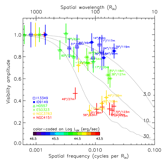
Figure 3: Observed mid-IR visibilities of all the targets, each averaged over 10 to 12 $\mu$m in the rest frame of each object, shown as a function of spatial frequency in units of cycles per $R_{\rm in}$ (log-scale). The data are color-coded in terms of the UV luminosity of the central engine for the corresponding object, which is defined to be 6 $\nu L_{\nu}$(5500Å) (Kishimoto et al. 2007). Each data point is plotted with different symbols for different objects, and is labeled with the PA / length of the baseline. It is quite clear that the radial structure in units of $R_{\rm in}$ changes from being compact in higher luminosity objects to extended in lower luminosity objects. Dotted curves are visibility functions for power-law brightness distribution with the normalized half-light radius $R_{\rm 1/2}/R_{\rm in}$=3, 10, and 30., which roughly depict the brightness distributions from higher to lower luminosity objects.

3.3 Mapping radial structure

Each panel of Figs.1 and 2 shares a common range of axes over different objects so that we can directly compare them. We can also place together the data for all the targets on a single plane. Fig.3 is such a figure, showing the observed mid-IR visibilities of all the targets, each averaged from 10 to 12 $\mu$m in the rest frame of each object. In Appendix C, we also show the same figure with the spatial frequency axis on a linear scale.

Our mid-IR observations cover the range of several tens to hundreds of $R_{\rm in}$ in spatial wavelengths. Over this range, the observed visibilities are relatively concentrated in one locus, from 0.3 to 0.9. If the visibilities of different objects followed the same curve, this would mean that the size scales only with $L^{1/2}$ and objects share the same radial structure as inferred by Kishimoto et al. (2009b). However, this is not the case.

In Fig. 3, each object is color-coded with its UV luminosity as defined in Sect.3.1. It is quite clear from the figure that within the small sample, which nevertheless spans over $\sim$2.5 orders of magnitudes in luminosity, the radial structure does depend on luminosity, i.e. the structure in units of $R_{\rm in}$ looks more compact in higher luminosity objects. This implies that the increase in the mid-IR physical size (e.g. in pc) with luminosity is more gradual than $L^{1/2}$. We discuss this luminosity dependence in Sect.4.1.

While the results above are essentially model-independent, we attempt in the following to describe the radial surface-brightness distribution more specifically with simple models. The dotted curves in Fig. 3 are visibility functions for power-law brightness distributions, which we argue below approximately depict the observed brightness distributions (see more in Sect.3.5).

3.4 Single Gaussian/ring versus power-law

We first consider the results for ESO323-G77, where we have the data with the least ambiguity. The total flux spectrum provides with an excellent match to the simultaneous VISIR spectrum (see Sect.2.3; Fig.20) and we have the two datasets at almost exactly the same PA of the baselines ($\sim$$38\degr$) with good S/N. The visibility data are shown in Fig.4 as a function of spatial frequency.

As in the middle panel of Figs. 1 and 2, the visibilities in Fig.4 are presented in different colors for different wavelengths as indicated by the color bar. For a given baseline, shorter wavelengths probe the source at higher spatial resolutions, and if the overall source size is the same when seen at different wavelengths, then the visibility is expected to become lower, i.e. more resolved, toward shorter wavelengths. However, the observed visibility spectra are roughly flat, or increase toward shorter wavelengths, which means that the overall size of the source is smaller at shorter wavelengths. This is also generally seen in other objects, except at some objects’ shortest wavelengths where visibilities might be slightly underestimated owing to a coherence loss (see Appendix A.4).

On the other hand, when we consider the visibilities at each wavelength as a function of baselines (or spatial frequencies), we can easily see that a simple Gaussian or ring (which we treat here almost equally, since they give almost identical visibility curves at low spatial frequencies well before the first null; see Sect.4.2 ) does not fit them well, as shown by the dotted and dashed Gaussian curves in the top panel of Fig.4. If we derive a Gaussian HWHM or ring radius for each baseline measurement at a fixed wavelength, we obtain a smaller size for longer baselines as we show in the bottom panel of Fig.4. We appear to observe here a brightness distribution where the corresponding Gaussian/ring sizes become progressively smaller at longer baselines. This probably means that there is a continuous distribution of brightness spread over a wide range of continuous spatial scales. This can be understood if the brightness distribution resembles a power-law distribution at a given wavelength, with its index generally becoming steeper at shorter wavelengths. This is what we advocated in Kishimoto et al. (2009b) (see their Fig.1). This power law is at least partially expected physically, since the temperature of the directly illuminated dust grains is expected to follow a power-law with the radius from the illumination source, simply based on thermal equilibrium (e.g. Barvainis 1987).

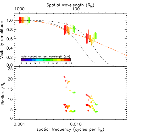
Figure 4: Top: Observed visibilities for ESO323-G77 as a function of spatial frequency along the position angle $\sim$$38\degr$. Visibility curves for Gaussian distributions with a HWHM/$R_{\rm in}$ of 20 (dotted) and 12 (dashed), and a power-law distribution with $R_{\rm 1/2}/R_{\rm in}=7$ (dash-dot) are over-plotted. Bottom: Gaussian HWHM (plus signs) and $R_{\rm 1/2}$ (filled circles) are plotted against the same spatial frequency. The red to green colors indicate the observing wavelengths in the rest frame from 13 to 8.5 $\mu$m. For a given wavelength, while the Gaussian HWHM is baseline-dependent, the half-light radius is approximately baseline-independent, thus seems adequate for representing the whole structure.

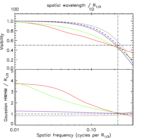
Figure 5: Top: Comparison between visibility functions for Gaussian, shown as a dashed curve, and power-law distributions where red, green, and purple curves correspond to the cases of $R_{\rm 1/2}$ = 6, 2, 1.3 $R_{\rm in}$, respectively. For comparison, the visibility function of a thin ring with radius being equal to the Gaussian HWHM (i.e. $R_{\rm 1/2}$) is shown as a dotted curve. Bottom: The ratio of Gaussian HWHM to $R_{\rm 1/2}$ is plotted against the same spatial frequency in each case. The vertical dot-dash line corresponds to the spatial wavelength of 4.5 $R_{\rm 1/2}$.

3.5 Half-light radius for power-law brightness distribution

For given inner and outer radii, a power-law index specifies a power-law brightness distribution, and a convenient way of characterizing the corresponding size is to use the half-light radius $R_{\rm 1/2}$, the radius within which half of the total integrated light at a given wavelength is contained. This can be directly compared with the HWHM of a Gaussian brightness distribution, since $R_{\rm 1/2}$ is equal to the HWHM in a Gaussian case. When the brightness distribution is adequately described by a power law, the values of $R_{\rm 1/2}$ derived from visibilities at different baselines should all be the same for a given wavelength. The bottom panel of Fig.4 presents the deduced $R_{\rm 1/2}$ for each visibility observed. We can see that the deduced $R_{\rm 1/2}$ is quite independent of the baseline lengths, in contrast to the Gaussian HWHM. This reassures that the power-law description in this case is quite adequate. We can also see that the size becomes smaller toward shorter wavelengths, as discussed above.

The disadvantage of adopting a power-law model and its corresponding $R_{\rm 1/2}$ is that we need to define both the inner and outer radii, which are set here to be 1$R_{\rm in}$ and 100$R_{\rm in}$, respectively. However, we can also define another, very similar, more model-independent radius, the half-visibility radius $R_{\rm V0.5}$ as follows. A visibility at a given low spatial frequency (within the first lobe of the visibility function before the first null) roughly corresponds to the fraction of the flux that is contained within the spatial scale being probed and remains unresolved by the interferometer’s configuration. Here the configuration is set by the observing wavelength $\lambda$ and baseline length $B$. In this sense, $R_{\rm 1/2}$ roughly corresponds to the spatial scale probed by the interferometer for which the visibility becomes 0.5. We can refer to this spatial scale using the spatial wavelength $\Lambda\equiv\lambda/B$, which is the reciprocal of the spatial frequency for the configuration, and corresponds to the spatial resolution of the configuration (Kishimoto et al. 2009b; see Sect.3.1). It is straightforward to show that the spatial wavelength $\Lambda_{0.5}$ at which visibility becomes 0.5 for a Gaussian is related to $R_{\rm 1/2}$ by

$$R_{\rm 1/2}=\frac{\ln 2}{\pi}\ \Lambda_{0.5}\ \ {\rm(for\ a\ Gaussian)}.$$ (2)

If we define the half-visibility radius $R_{\rm V0.5}$ as

$$R_{\rm V0.5}\equiv\frac{\ln 2}{\pi}\ \Lambda_{0.5}\simeq\frac{\Lambda_{0.5}}{4.5},$$ (3)

then this is equal to $R_{\rm 1/2}$ for a Gaussian, and can generally be referred to as a good approximation of the half-light radius model-independently. This radius can approximately be deduced by interpolating observations when observed visibilities cross over 0.5 at the longest available baseline. We can also say more generically that the visibility at a given spatial wavelength $\Lambda$ within the first lobe gives the approximate fraction of flux originating from the region within the radius $\sim$$\Lambda/4.5$. We note again that for a Gaussian brightness distribution, all three quantities, namely HWHM, half-light radius $R_{\rm 1/2}$ and half-visibility radius $R_{\rm V0.5}$, are identical.

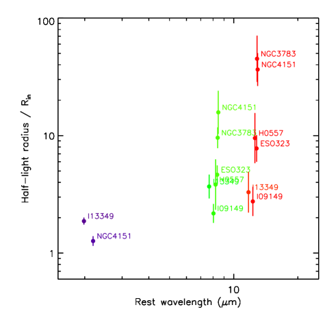
Figure 6: Normalized half-light radii $R_{\rm 1/2}/R_{\rm in}$ plotted against rest wavelengths. Thin-ring radii at 2.2$\mu$m, normalized by $R_{\rm in}$, from the KI data for two objects (Kishimoto et al. 2009a) are also shown. The normalized radii become smaller for shorter wavelengths in each object from the mid-IR to near-IR.

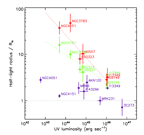
Figure 7: Normalized half-light radii $R_{\rm 1/2}/R_{\rm in}$ (red and green for 13 and 8.5 $\mu$m, respectively), plotted against UV luminosity $L$, defined as 6 $\nu L_{\nu}$(5500Å) (Kishimoto et al. 2007). The red and green dotted lines are power-law fits to $R_{\rm 1/2}/R_{\rm in}$ at 13 $\mu$m and 8.5 $\mu$m, respectively. The normalized radii become more compact in the objects having the central engine with a higher UV luminosity. Also shown in purple are thin-ring radii at 2.2 $\mu$m normalized by $R_{\rm in}$ for the sample observed with the KI (Kishimoto et al. 2011), including two overlapping objects. The gray dotted horizontal line indicates radius = $R_{\rm in}$.

Table 6: Estimated half-light radii $R_{\rm 1/2}$ in two rest-frame wavelengths in the mid-IR and their uncertainties in dex.

name	$R_{\rm in}$a	8.5 $\mu$m			13 $\mu$m
	(pc)	$R_{\rm 1/2}/R_{\rm in}$	$R_{\rm 1/2}$ (pc)	unc. (dex)	$R_{\rm 1/2}/R_{\rm in}$	$R_{\rm 1/2}$ (pc)	unc. (dex)
NGC4151	0.033	15.9	0.52	0.18	36.8	1.21	0.14
NGC3783	0.061	10.0	0.60	0.09	46.9	2.84	0.20
ESO323	0.10	4.7	0.49	0.08	7.9	0.83	0.12
H0557-385	0.12	4.1	0.51	0.21	10.2	1.26	0.21
IRAS09149	0.47	2.2	1.06	0.09	2.8	1.33	0.13
IRAS13349	0.49	3.6	1.76	0.12	3.2	1.58	0.20

^a See Table 1 for $R_{\rm in}$ ($\equiv R_{\rm\tau_{K}}$ fit) in mas.

In the top panel of Fig.5, we compare the visibility functions of Gaussian and power-law distributions with various $R_{\rm 1/2}$. The curves are shown as a function of spatial frequency in units of cycles per $R_{\rm 1/2}$ (or spatial wavelength in units of $R_{\rm 1/2}$), so that we can directly compare different $R_{\rm 1/2}$ power-law cases with the same Gaussian curve. We can see that power-law curves with smaller values of $R_{\rm 1/2}$ become asymptotically more similar to the Gaussian/ring curve. The bottom panel shows the ratio of Gaussian HWHM, derived from each visibility, to $R_{\rm 1/2}$ as a function of the same spatial frequency. For extended power-law distributions, the dependence of the Gaussian HWHM on the baseline length is quite strong, but for steep distributions, the dependence on baseline becomes quite small. All curves cross the visibility $V$ of 0.5 at spatial wavelength $\Lambda$ close to 4.5 $R_{\rm 1/2}$, meaning that the half-visibility radius $R_{\rm V0.5}$ closely represents the half-light radius $R_{\rm 1/2}$ in all cases.

The dotted curves in Fig. 3 are the visibility functions for the power-law brightness distributions with three different steepnesses, which are quantified by the normalized half-light radius $R_{\rm 1/2}/R_{\rm in}$=3, 10, and 30 (corresponding to power-law indices of -2.6, -2.0, and -1.5, respectively). These seem to closely describe the mid-IR surface brightness distribution over the sample. For the more compact structures seen in the higher luminosity objects, it is more difficult to differentiate the power-law from a Gaussian/ring for a given measurement uncertainty. However, based on relatively resolved cases such as in ESO323-G77, we infer that the power-law description with different values of $R_{\rm 1/2}$ over the sample is adequate at least approximately. We can then translate the observed visibility curves on the 2D plane (Fig.3, or the middle panels of Figs.1 and 2) into a value of $R_{\rm 1/2}$ at each wavelength, and then disscuss the relation between this size information and other observables.

We derived the best-fit normalized half-light radius $R_{\rm 1/2}/R_{\rm in}$ for each object by fitting the visibility curve of a power-law brightness distribution to the observed visibility data, separately for four wavelength bins, namely 8.2-10, 10-11, 11-12, and 12-13 $\mu$m in the observed frame. To ensure a uniform comparison at the same rest wavelength over the sample, we fitted a power law as a function of wavelength over the derived $R_{\rm 1/2}/R_{\rm in}$ (and its error) at the four wavelength bins, and used this fit to derive values at 8.5 and 13 $\mu$m in the rest frame. The results are summarized in Table 6. The uncertainties are formal 1-$\sigma$ uncertainties for the fits, except for NGC4151 and NGC3783 where the targets are well-resolved ($V<0.5$ at long baselines) and the uncertainty in $R_{\rm 1/2}$ was estimated as the dispersion in those derived from different baseline data. Since the dispersion in $R_{\rm 1/2}$ about its best-fit value was more symmetric in log space, the uncertainties are shown in dex.

We note that the fits were done with the inner and outer radius fixed at 1 and 100 $R_{\rm in}$. The latter can affect the radius estimation for the extended cases of NGC4151 and NGC3783. However, as long as each source is at least approximately unresolved by the single telescope, the half-visibility radius $R_{\rm V0.5}$ is quite well-constrained as can be seen in the middle panels of Fig.1$a$ and Fig.1$b$ as well as in Fig.3 (see Sect.3.2). Therefore, our $R_{\rm 1/2}$ estimation would also be quite robust for the two targets.

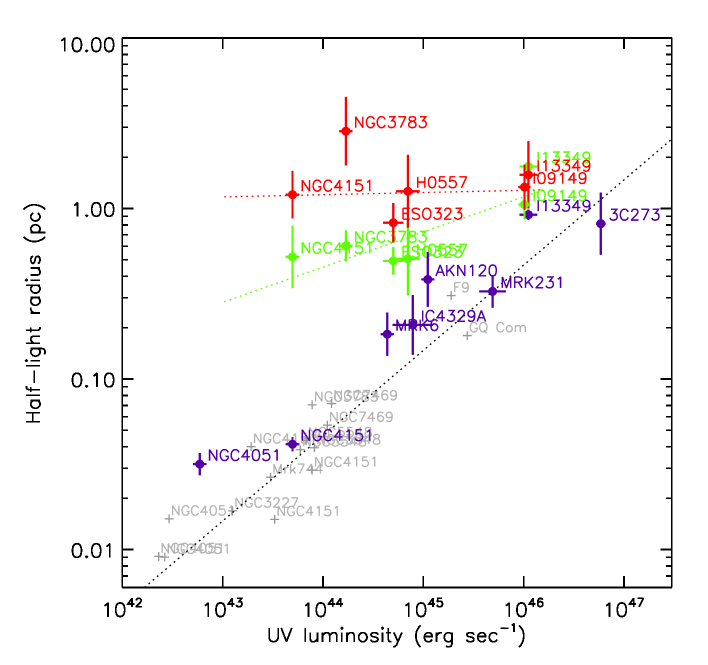
Figure 8: Half-light radii $R_{\rm 1/2}$ in pc (red and green for 13 and 8.5 $\mu$m, respectively), plotted against UV luminosity $L$, which is defined as 6 $\nu L_{\nu}$(5500Å) (Kishimoto et al. 2007). The red and green dotted lines are power-law fit to $R_{\rm 1/2}$ at 13$\mu$m ($\propto L^{0.01\pm 0.07}$) and 8.5$\mu$m ($\propto L^{0.21\pm 0.05}$), respectively. In this physical scale, these mid-IR radii increases with luminosity much slower than $L^{1/2}$, or almost constant at 13 $\mu$m. Thin-ring radii at 2.2$\mu$m also in pc are plotted in purple for the KI-observed sample. Plotted with gray plus signs are the near-IR reverberation radii (Suganuma et al. 2006 and references therein), with the black dotted line showing their $L^{1/2}$ fit. This fit is the definition of the inner radius $R_{\rm in}$ in this paper.

4 Discussion

4.1 Sizes at various wavelengths as a function of UV luminosity

Using the half-light radius $R_{\rm 1/2}$ derived in the previous section, we discuss below the overall relations of the size to observing wavelengths and flux-related quantities such as spectral shape, total flux, and luminosity.

Fig.6 shows $R_{\rm 1/2}/R_{\rm in}$ as a function of rest-frame wavelengths. For the near-IR, we have plotted the thin-ring radii from the KI data for the two objects in our present MIDI sample, NGC4151 and IRAS13349 (Kishimoto et al. 2009a). The thin-ring approximation should be fairly robust in the near-IR, where the radial brightness distribution is expected to be much steeper and the power-law visibility curve becomes very close to that of a Gaussian/ring (Fig.5). A more detailed estimation of $R_{\rm 1/2}$ would require knowledge of the shape of the innermost dust distribution, which is not yet well constrained. Thus, we simply adopt here the thin-ring approximation for the near-IR data. We would infer that the other four targets, for which no KI data are available, probably have near-IR ring radii of $\sim$1$-$2 $R_{\rm in}$ based on the KI-observed sample of type 1 AGNs (see Fig.7; Kishimoto et al. 2011). From the mid-IR to the near-IR, the normalized emission size would then become certainly smaller with wavelength, very roughly following some power law for each object, but with different indices for different objects.

As we demonstrated in Fig.3, the mid-IR emission size seems to have a luminosity dependence. This is now quantitatively shown in Fig.7, where $R_{\rm 1/2}/R_{\rm in}$ is plotted against UV luminosity $L$. The data points are color-coded for the observing wavelengths, and we include the 2.2 $\mu$m thin-ring radii of all the KI-observed sample from Kishimoto et al. (2011). As we can see, the ratio of half-light radius to $R_{\rm in}$ becomes smaller with increasing UV luminosity. This implies that, for a given radial temperature distribution, the higher luminosity objects have a steeper radial density structure, at least in the mid-IR emitting radii, as we discuss in greater detail below. We also plot power-law fits to the $R_{\rm 1/2}/R_{\rm in}$ at 8.5 and 13 $\mu$m in Fig.7.

We can also analyze the luminosity dependence of unnormalized $R_{\rm 1/2}$ in a physical scale. Fig.8 shows the half-light radius $R_{\rm 1/2}$ in pc plotted against the same UV luminosity. In the physical scale, the radius in the mid-IR increases with luminosity much slower than $L^{1/2}$. Power-law fits to $R_{\rm 1/2}$ in pc at 8.5 and 13 $\mu$m as a function of luminosities are

$$R_{\rm 1/2}\ (8.5\mu{\rm m})=(1.2\pm 0.2)\cdot\left(\frac{6\nu L_{\nu}(5500\AA)}{10^{46}\ {\rm erg/sec}}\right)^{0.21\pm 0.05}\ {\rm pc},$$ (4)

and

$$R_{\rm 1/2}\ (13\mu{\rm m})=(1.3\pm 0.3)\cdot\left(\frac{6\nu L_{\nu}(5500\AA)}{10^{46}\ {\rm erg/sec}}\right)^{0.01\pm 0.07}\ {\rm pc},$$ (5)

where we see that $R_{\rm 1/2}$ at 13 $\mu$m is consistent with being constant.

These results are contrary to those of previous studies of the mid-IR size as a function of luminosity by Tristram et al. (2009) and Tristram & Schartmann (2011), who concluded that the mid-IR size is consistent with being proportional to $L^{1/2}$. They used a single Gaussian for the size estimation, and this can lead to a large systematic error owing to the baseline dependency. When the radial brightness distribution has a relatively shallow power-law form, a Gaussian size would represent the emission size that is resolved by a given interferometer configuration, leading to the strong dependence on the sampled $uv$ points. Thus, in this case, the simple Gaussian size is quite inadequate for representing the emission size for the whole distribution. Here we account for the effect of the $uv$ sampling more properly, based on the inference that the brightness distribution is of roughly a power-law form. This enables us to perform a more accurate, uniform comparison over the sample, as shown in Fig.8. To gain a greater accuracy and model-independency, we can always return to the uniform view of the visibility curves over the sample shown in Fig.3.

The half-light radius in units of $R_{\rm in}$ has a quite close relationship with the mid-IR spectral shape. Figure 9 shows $R_{\rm 1/2}/R_{\rm in}$ plotted against spectral index $a$ in $f_{\nu}\propto\nu^{a}$ in the mid-IR. The shape becomes bluer when the size is smaller. In terms of the radial structure, this is what we would expect, as the steeper radial structure looks bluer as the contribution from hotter dust becomes more dominant. We elaborate on this point later using simple models.

We can also calculate an average surface brightness in the rest frame using $R_{\rm 1/2}$ as $(\nu L_{\nu}/4\pi)/(\pi R_{\rm 1/2}^{2})$, which is equivalent to $\nu_{\rm obs}f_{\nu_{\rm obs}}\cdot(1+z)^{4}/(\pi\theta_{1/2}^{2})$ where $\theta_{1/2}$ is the angular size of $R_{\rm 1/2}$. Fig.10 shows this as a function of rest-frame wavelengths. This can be directly compared with the Planck function as shown in the same figure, where the comparison gives the brightness temperature at a given wavelength. In the near-IR, all the objects show the brightness temperature $\sim$1400$-$1000K, while in the mid-IR the brightness temperature ranges from $\sim$1000K to $\sim$200K. In the near-IR, the brightness temperature is quite close to the observed color temperature of $\sim$1400K, meaning that the average surface filling factor at the innermost dusty region must be close to unity. Figure 11 shows the surface brightness as a function of UV luminosity, and the corresponding brightness temperatures at 2.2 and 13 $\mu$m are shown in the second and third y-axis, respectively. We can again clearly see the luminosity dependence.

The close relationship between $R_{\rm 1/2}/R_{\rm in}$ and the mid-IR spectral index (Fig.9) and the relationship between $R_{\rm 1/2}/R_{\rm in}$ and UV luminosity (Fig.7) implies that there should also be a correlation between the mid-IR spectral index and luminosity. In fact, the luminosity dependence of the radial dust distribution was already inferred by Hönig et al. (2010), based on the IR spectral comparison between Seyfert galaxies and high-luminosity type 2 QSOs. Here we directly show the distribution change by spatially resolving it.

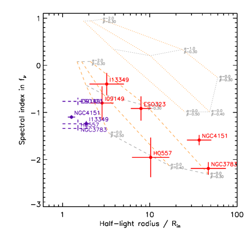
Figure 9: The mid-IR (8.5$-$13 $\mu$m) spectral indices in $f_{\nu}$ are plotted in red against normalized half-light radii $R_{\rm 1/2}/R_{\rm in}$ at 13 $\mu$m. Also plotted in purple are spectral indices between 2.2 and 13 $\mu$m against thin-ring radii at 2.2 $\mu$m normalized by $R_{\rm in}$. For the four objects without near-IR interferometry data, we indicated the near- to mid-IR spectral indices in dashed lines over the thin-ring radius range of 1$-$2 $R_{\rm in}$, roughly expected based on other targets observed with the Keck interferometer (see Fig.7). The dotted line shows the grid for a simple power-law model with radial surface density index $\alpha$ of (-2.0, -1.0, -0.0) and temperature index $\beta$ of (-0.5, -0.4, -0.3) with the innermost tempeture $T_{\rm in}$=1400K. The grid covers the observed range of $R_{\rm 1/2}/R_{\rm in}$, but systematically bluer in spectral shape. The dashed lines show the same grid but with $T_{\rm in}$=700K, which apparently matches the mid-IR observations over the sample when the density index ranges from $\sim$$-1$ to 0 in different objects with a temperature index of $\sim$$-0.35\pm 0.05$ (for details, see Sect.4.4).

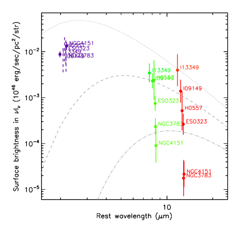
Figure 10: Average surface brightnesses $\nu I_{\nu}$ in the rest frame, defined as $(\nu L_{\nu}/4\pi)/(\pi R_{\rm 1/2}^{2})$, are plotted against rest wavelengths. Overplotted are the Planck functions with temperatures 1400, 700, and 350 K (dotted, dashed, and dash-dot, respectively). For NGC4151 and IRAS13349, which have near-IR Keck interferometry data, the average surface brightness at 2.2 $\mu$m is calculated in the same way but using thin-ring radii. For the objects without near-IR interferometry, it is calculated assuming $R_{\rm 1/2}$=(1.5$\pm$0.5) $R_{\rm in}$ and indicated by dashed lines. See further details in Sect.4.1.

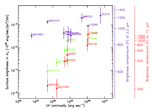
Figure 11: The same average surface brightness as in Fig.10, but plotted against the UV luminosity of the central engine, defined as 6 $\nu L_{\nu}$(5500Å) (Kishimoto et al. 2007). The red and green symbols correspond to 13 and 8.5 $\mu$m, respectively. The surface brightness at 2.2 $\mu$m is shown in purple for those with the near-IR interferometry data from Kishimoto et al. (2011). The luminosity dependence is quite clear at least for the surface brightness in the mid-IR.

Table 7: The results of two-temperature Gaussian fits.

name	$R_{\rm in}$b	near-IR Gaussian			mid-IR Gaussian			$\chi_{\nu}^{2}$ (c)	minor/major
	(pc)	T(K)	HWHM ($R_{\rm in}$)	$f_{0}$	T(K)	HWHM ($R_{\rm in}$)	$f_{0}$
NGC4151	0.033	1389$\pm$68	1.06$\pm$0.02	0.36$\pm$0.10	282$\pm$6	51.1$\pm$1.2	0.12$\pm$0.01	12.9
NGC3783	0.061	1220$\pm$108	(fixed to 1)	0.57$\pm$0.28	242$\pm$9	32.4$\pm$0.6	0.77$\pm$0.14	8.1
NGC3783a	0.061	1220$\pm$108	(fixed to 1)	0.57$\pm$0.28	242$\pm$9	39.5$\pm$1.0	1.12$\pm$0.21	4.1	0.46$\pm$0.02
ESO323	0.10	1539$\pm$175	(fixed to 1)	0.29$\pm$0.14	320$\pm$18	12.3$\pm$0.4	0.71$\pm$0.15	1.7
H0557-385	0.12	1241$\pm$54	(fixed to 1)	0.97$\pm$0.26	307$\pm$15	18.2$\pm$1.2	1.06$\pm$0.26	1.4
IRAS09149	0.47	1204$\pm$103	(fixed to 1)	0.63$\pm$0.32	290$\pm$39	7.4$\pm$0.5	1.67$\pm$0.89	0.65
IRAS13349	0.49	1314$\pm$57	1.57$\pm$0.06	0.37$\pm$0.10	366$\pm$26	9.6$\pm$0.7	1.9$\pm$0.6	0.98

^a An elliptical Gaussian is fit for the mid-IR component, assuming the major axis at 136°. The quoted mid-IR HWHM is along this major axis.
^b See Table 1 for $R_{\rm in}$ ($\equiv R_{\rm\tau_{K}}$ fit) in mas. ^c Reduced $\chi^{2}$ values for visibility fits.

4.2 Multiple-temperature Gaussian fit

While the power-law brightness description at each wavelength gives a relatively model-independent measurement of the emission size, it does not physically describe the change in the overall size with wavelength and the flux that we observe. A simple, though very approximate way of describing the power-law brightness with changing steepness over different wavelenths is to consider two or more rings/Gaussians of different size at different temperatures. At each wavelength, the multiple components with different sizes contribute differently to the visibility function, giving a wider range in spatial frequency than the range covered by a single ring/Gaussian. The contribution ratio of the multiple temperature components changes with wavelength, causing the overall apparent size to change with wavelength.

We adopted a Gaussian geometry for each component, though rings might provide a more physically accurate description of in particular the innermost dusty region. In terms of the visibility function, a ring and Gaussian essentially give the same curve at the low spatial frequencies before the first null (Fig.5; see e.g. Millour 2008). Both a thin-ring and a Gaussian geometry have only one parameter, but a Gaussian permits us to more simply quantify the average surface brightness of the component, and its visibility curve (which is also a Gaussian) is the simplest (no nulls, no lobes).

We describe each Gaussian component as a brightness distribution $S_{\nu}$ at a radius $r$ from the center given as

$$S_{\nu}(\nu,r)=B_{\nu}(\nu,T)\cdot f_{0}\ln 2\cdot e^{-r^{2}\ln 2/R_{\rm 1/2}^{2}},$$ (6)

where $B_{\nu}$ is the Planck function at frequency $\nu$ and temperature $T$, and $R_{\rm 1/2}$ is the physical size of the Gaussian in HWHM, where HWHM = $R_{\rm 1/2}$ for Gaussian. The isotropic luminosity $L_{\nu}$ of this component is

$$L_{\nu}/4\pi=f_{0}\cdot B_{\nu}(\nu,T)\cdot\pi R_{\rm 1/2}^{2}.$$ (7)

The factor $f_{0}$ gives the average surface brightness with respect to the blackbody when all the emission is contained within HWHM (see more on emissivity and surface filling factor described in Sect.4.4). In addition to these two Gaussians, we also include the accretion disk component, which is assumed to remain unresolved and have a spectrum of $f_{\nu}\propto\nu^{+1/3}$ at IR wavelengths longward of 0.8 $\mu$m (Kishimoto et al. 2009a, 2008).

Table 7 shows the results of two-Gaussian-component fits. We assumed that HWHM=1$R_{\rm in}$ for the $\sim$1400K near-IR component here, except for the two objects for which we have KI data. We see that the $\sim$300K mid-IR component has a HWHH of several to a few tens of $R_{\rm in}$, which implies an effective temperature radial gradient of $\beta$ from $\sim$$-0.8$ to $\sim$$-0.4$ where $T\propto r^{\beta}$. This effective index includes the effect of the radial gradient of surface density distribution. In section 4.4, we attempt to separate the temperature and density gradients using more physical but simple models.

4.3 PA dependence

The PA coverage of our baselines for each object is very limited. Since our targets are all type 1 AGNs, we do not expect to see a large PA dependence in visibilities. Nevertheless, we seem to see some PA dependence at least in one object, NGC3783. This has already been pointed out by Hönig et al. (2010). The brightness distribution along the SE-NW direction seems more extended than that in the NE-SW direction.

We can complement our inner PA dependency study with optical polarization measurements. The projected direction of the system polar axis can be inferred to be either parallel or perpendicular to the PA of the optical continuum polarization, depending on the line polarization properties (Smith et al. 2004; Kishimoto et al. 2004). If a linear radio structure is detected, this direction also indicates that of the system polar axis. All the targets except IRAS09149 have optical polarization measurements (Brindle et al. 1990; Wills et al. 1992; Martel 1998; Schmid et al. 2003), and a clear radio axis is also available for NGC4151 (Mundell et al. 2003). The resulting inferred PAs are summarized in Table 5, and shown in the bottom panel of the $uv$ coverage for each object in Fig.1 and 2 with polar and equatorial directions in dashed and solid lines, respectively.

To evaluate the elongation of the mid-IR emission in NGC3783, we attempted to fit an elliptical Gaussian for the mid-IR component with the major axis fixed at the polar axis PA 136°, and the results are listed in Table7. The emission seems to be a factor of $\sim$2 elongated along this polar direction, suggesting that some of the mid-IR emission originates from the polar region. More extensive data and analyses will be presented for this object by Hönig et al. (2011 in prep).

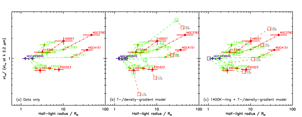
Figure 12: (a) SED in $\nu L_{\nu}$ for each object normalized at $\lambda$ = 2.2 $\mu$m, plotted against normalized half-light radius $R_{\rm 1/2}/R_{\rm in}$, for 2.2, 8.5, and 13 $\mu$m (purple, green, and red, respectively). (b) The same data but with the grid in dashed lines for temperature/density gradient models with radial surface density indices of $\alpha$=$-$0.4,$-$0.8,$-$1.2,$-$1.6 for the case of $T\propto r^{-0.36}$, plotted for the three wavelengths 2.2, 8.5, and 13 $\mu$m (purple, green, and red squares). This simple power-law model does not explain the observed SED and size at the same time. (c) The same data but with the grid in dashed lines for the power-law (density $\propto r^{-0,-0.2,-0.4,-0.6}$, $T\propto r^{-0.36}$) + 1400K thin-ring at $R_{\rm in}$, which roughly explain the observed SED and size. The two reddened sources IRAS13349 and H0557-385 could be interpreted in terms of the same model with a slightly larger filling factor for the power-law component.

Table 8: The fit results of temerature/density gradient model + inner ring.

name	power-law ($T_{\rm in}=700$ K)			inner 1400K ring		$\chi_{\nu}^{2}$	polar /
	density index $\alpha$	$T$ index $\beta$	$f_{0}$	radius ($R_{\rm in}$)	$f_{0}$		equatorial
NGC4151	$-0.31\pm 0.04$	$-0.26\pm 0.01$	$0.16\pm 0.01$	$1.25\pm 0.03$	$0.26\pm 0.02$	3.5
NGC3783	$+0.04\pm 0.05$	$-0.31\pm 0.01$	$0.16\pm 0.02$	(fixed to 1)	$0.29\pm 0.02$	2.4
NGC3783a	$+0.04\pm 0.06$	$-0.35\pm 0.01$	$0.13\pm 0.02$	(fixed to 1)	$0.28\pm 0.02$	0.69	$2.43\pm 0.18$
ESO323-G77	$-0.77\pm 0.09$	$-0.30\pm 0.02$	$0.55\pm 0.09$	(fixed to 1)	$0.42\pm 0.03$	0.60
H0557-385	$-0.65\pm 0.10$	$-0.31\pm 0.02$	$1.40\pm 0.26$	(fixed to 1)	$0.47\pm 0.02$	1.3
IRAS09149	$-0.46\pm 0.21$	$-0.42\pm 0.03$	$0.69\pm 0.19$	(fixed to 1)	$0.27\pm 0.02$	0.68
IRAS13349	$-1.26\pm 0.16$	$-0.27\pm 0.03$	$3.6\pm 1.0$	$1.87\pm 0.07$	$0.17\pm 0.01$	0.71

^a Fit with additional ellipticity for power-law component, assuming polar axis at 136°.

4.4 Power-law brightness distribution: temperature/density-gradient model

4.4.1 Model description

We now discuss the direct physical constraints on the radial structure of the inner dusty region thermally emitting in the IR. To this end, we use a simple but generic description of the radial surface brightness distribution with as few parameters as possible. To physically describe a face-on radial brightness distribution $S_{\nu}(\nu,r)$ at radius $r$ and observing frequency $\nu$, we would need at least two separate distributions, namely the temperature and surface density distributions. Here we slightly generalize the surface brightness description in Kishimoto et al. (2009b) as

$$S_{\nu}(\nu,r)=f_{\varepsilon}(r)\cdot B_{\nu}(\nu,T_{\rm max}(r)).$$ (8)

The idea behind this description is that, at each radius, the face-on surface brightness is dominated by the emission from the heated dust grains that have a maximum temperature at that radius (e.g. Hönig & Kishimoto 2010). These grains are probably at around the surface of the torus, and most likely directly illuminated by the central source, if there are such directly illuminated grains at that radius. Under this maximum-temperature approximation, we refer to the dust at $T_{\rm max}$ simply as heated dust grains/clouds. We note that our observations are insensitive to much colder, interior dust grains that may exist deeper along our line of sight at that radius. We write this maximum temperature $T_{\rm max}(r)$ at radius $r$ as

$$T_{\rm max}=T_{\rm in}\cdot(r/R_{\rm in})^{\beta}.$$ (9)

We mainly consider a discrete, clumpy, or inhomogeneous cloud distribution. The surface brightness of each heated cloud at radius $r$ would approximately scale with $r$ in proportion to $B_{\nu}(T_{\rm max}(r))$. The additional factor $f_{\varepsilon}(r)$ above, which we write in the form of a power law as

$$f_{\varepsilon}(r)=f_{0}\cdot(r/R_{\rm in})^{\alpha},$$ (10)

describes the radial run of the surface density (i.e. per unit area) distribution of these heated discrete clouds (i.e. at $T_{\rm max}$), but also includes the emissivity of each heated cloud surface. More specifically, the dimensionless factor $f_{\varepsilon}$ can be regarded as a surface filling factor multiplied by the emissivity. In the case of optically thick illuminated clouds where their emissivity does not depend sensitively on the radial distance from the illuminating source or the observing frequency (e.g. Hönig & Kishimoto 2010, see their Fig.3), the factor $f_{\varepsilon}(r)$ is roughly proportional to the radial surface density distribution of the heated clouds, or heated dust grains. Thus, as long as the emissivity is roughly constant over the radius and frequency, we can regard $f_{\varepsilon}(r)$ as a normalized surface density of heated dust grains (i.e. again those at $T_{\rm max}$). In this way, our description is generic enough to ensure that we can obtain as direct constraints as possible from the observations.

The model would be called a temperature gradient model, if the density distribution is set to be uniform, i.e. $\alpha=0$, and the brightness described only by the temperature index $\beta$. In this case, the index would be an effective temperature index, which would include the effect of the density gradient. Here we try to separate the temperature and density gradient. At least in the case of the direct illumination of a dust grain, we would expect that $\beta$=$-0.5$ for large grains and $\beta$$\sim$$-0.36$ for standard-size ISM grains (e.g. Barvainis 1987). By referring to these values, we attempt here to obtain constraints on the surface density distribution.

4.4.2 Mid-IR spectral slope and SED-size relation

In Fig.9, we show a grid for the two indices $\alpha$ and $\beta$ on the plane of the mid-IR spectral index and half-light radius. The upper-most grid with dotted lines is for $T_{\rm in}=1400$K, which corresponds to the observed color temperature in the near-IR and is thought to be roughly equal to the dust sublimation temperature. The range of density index $\alpha$ from $-$2 to 0 for a given temperature index reproduces the observed range of normalized half-light radii $R_{\rm 1/2}/R_{\rm in}$. However, the expected mid-IR spectral shape as shown by the dotted grid is systematically bluer than observed. In fact, the observed range of the mid-IR spectral index, as well as that of $R_{\rm 1/2}/R_{\rm in}$, is reproduced well with the power-law distribution if $T_{\rm in}$ is $\sim 700$K, where the corresponding grid is shown in dashed lines in Fig.9. We need to accommodate this size-color constraint.

The total flux spectra, including the mid-IR spectral shape, and the size information for all the objects can be summarized on the plane of the SED, normalized at 2.2 $\mu$m where all objects show similar brightness temperature (Fig.10), plotted against $R_{\rm 1/2}/R_{\rm in}$ as shown in Fig.12$a$. For objects without Keck near-IR interferometric data, we set their $R_{\rm 1/2}$ at 2.2 $\mu$m to have the expected range of values from 1 to 2 $R_{\rm in}$ (see Fig.7; Kishimoto et al. 2011). In the mid-IR, the objects show a relatively uniform behavior. From the high to low luminosity objects, as the normalized size $R_{\rm 1/2}/R_{\rm in}$ becomes larger, the mid-IR spectral shape becomes gradually redder (which is already seen in Fig.9), and the mid-IR total flux level gradually increases with respect to the near-IR flux, although two objects, IRAS13349 and H0557-385, seem to have slightly (a factor of a few) higher mid-IR flux level than the other four objects (see more below).

Overplotted in dashed lines in Fig.12$b$ on the same data set is the SED-size relation at three wavelengths expected from the power-law distribution with the temperature index $\beta$=$-0.36$ over the range of density indices $\alpha$=$-$1.6 to $-$0.4 (the case with slightly steeper $\beta$ is similar, but with a slightly different density index range). The total flux mismatch can be clearly seen across this plane. It is quite difficult to reproduce the wide range of $R_{\rm 1/2}/R_{\rm in}$ and the overall near- to mid-IR SED which is relatively flat in $\nu f_{\nu}$, while keeping the relatively red mid-IR spectral shape, for this single power-law structure.

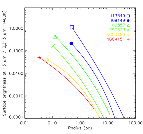
Figure 13: The modeled surface brightness distribution of the power-law component at 13 $\mu$m as a function of radius in pc. The value is normalized with the constant value of the Planck function at 13 $\mu$m for $T$=1400K. The color indicates the UV luminosity of each object as in Fig.3, which illustrates that higher luminosity objects have steeper and brighter surface brightness.

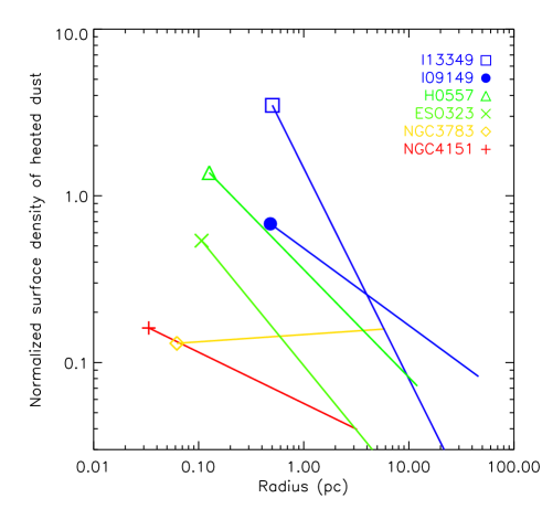
Figure 14: The modeled surface density distribution of heated dust (at maximum temperature at each radius) in the power-law component, illustrating that higher luminosity objects have steeper and denser distributions.

4.4.3 Mapping the radial structure with a bright near-IR rim

However, we would be able to roughly understand both the total flux and size information if, in addition to the power-law structure, there is a central brightness concentration on the scale of $\sim$$R_{\rm in}$ emitting nearly at the sublimation temperature of $\sim$1400K. This concentration would correspond to a dust sublimation region, and could be a bright rim of the innermost dust distribution, such as the puffed-up rim that is often discussed for the inner region of young stellar objects (see Dullemond & Monnier 2010 for a review). The exact structure of this central concentration is not yet well constrained with our data. Fig.12$c$ shows a grid of models with the power-law plus the central concentration represented simply by a 1400K ring at $r$=$R_{\rm in}$, which seems to closely reproduce the overall SED-size relation with a range of density indices. In this case, the two objects, IRAS13349 and H0557-385, simply have a slightly higher flux level in the power-law component with respect to the near-IR ring.

In Figures 1 and 2, we also show the best-fit results with this model for each object and Table 8 summarizes the parameters. The normalization of the ring luminosity is parameterized in the same way as in the case of Gaussian given in Eq.7, where $R_{\rm 1/2}$ is replaced by the radius of the ring. Figure 13 shows the resulting surface brightness profiles of the models for each object. The power-law component in higher luminosity objects becomes steeper, as expected. Figure 14 shows the corresponding normalized surface density distribution of the heated dust grains (i.e. with a maximum temperature at each radius). It becomes steeper, and also slightly denser, for higher luminosity objects. The density indices are from $\sim$0 for lower luminosity to $\sim$$-$1 for higher luminosity objects in our sample.

We note that the central temperature $T_{\rm in}$ of the mid-IR power-law distribution has to be as low as $\sim$700 K, to reproduce the relatively red mid-IR spectral shape. (We fixed $T_{\rm in}$ to be 700K in the fits implemented above, and we would need visibility data that fill the gap between near-IR and mid-IR wavelengths to constrain $T_{\rm in}$ more tightly.) This would mean that there is a compact region of such a low temperature quite close to the radius $R_{\rm in}$, which could be the shadowed region just behind the bright sublimating rim.

4.4.4 NGC4151

In the case of NGC4151, this low-temperature compact region is probably what we see in the mid-IR visibility curves, which become relatively flat at spatial wavelengths smaller than $\sim$100 $R_{\rm in}$ as shown in the mid-panel of Fig.1$a$. In our interpretation, this is caused by both the high spatial frequency part of the low-$T_{\rm in}$ power-law component and the hot central brightness concentration. Here the effect of the latter on visibility is indicated in this panel (also in the other mid-panels in Fig.1 and 2 for other objects), where the dotted curves show the visibilities without the bright near-IR rim.

These can also be understood in terms of the correlated flux observed at long baselines (see the top-panel of Fig.1$a$), which provides an approximate spectrum of the unresolved part of the source. Its color temperature is $\sim$400 K (or $\sim$500 K if we exclude slightly less reliable data at wavelengths shortward of $\sim$10 $\mu$m), which is much higher than that of the total flux ($\sim$280 K) and much lower than the sublimation temperature.

The deviation of our model fit from the data might indicate that the low-$T_{\rm in}$ core has even more flux while the outer radiating source is even more extended. This could suggest a model of three components (including the near-IR component), which was implied by Burtscher et al. (2009), who modeled their two-baseline mid-IR data with a Gaussian and an unresolved source, and suggested another near-IR component. We note, however, that, puzzlingly, the correlated flux in their two-baseline data did not show the relatively blue color temperature, thus gave almost no indication of the size becoming smaller toward shorter wavelengths within the mid-IR.

4.4.5 Warm mid-IR and hot near-IR parts

The composite brightness structure discussed above, consisting of emission components of a warm mid-IR dominating part and a hot near-IR dominating part, also seems to be discernible in the SED, particularly in those of relatively red objects such as NGC3783 and NGC4151 (Fig.1). The two-component explanation of the near to mid-IR SEDs has been advocated by different authors from SED analyses (e.g. Mor et al. 2009). Historically, the bump around 3 $\mu$m in the SEDs of QSOs, which could correspond to the hot near-IR part, has been known for decades (e.g. see sec.V in Neugebauer et al. 1979).

A direct size constraint on the hot central brightness concentration can be derived from near-IR interferometry, and its structure might be a little distinct from the warm power-law distribution. For example, the near-IR visibility of NGC4151 suggests that it has a quite compact structure with $R_{\rm 1/2}$ quite close to $R_{\rm in}$, while most of its mid-IR emission is quite extended. In that case, another parameter, in addition to the heating luminosity, may be responsible for forming the structure of the inner region. We plan to explore these regions with further measurements in both the near-IR and mid-IR.

5 Conclusions

We have presented mid-IR long-baseline interferometry of six type 1 AGNs. Within the small sample, which nevertheless spans over $\sim$2.5 orders of magnitudes in the UV luminosity $L$ of the central engine, we have shown that the radial structure of the dust distribution changes systematically with luminosity. We have argued that the mid-IR radial brightness distribution can approximately be described by a power-law with the inner boundary set by the dust sublimation radius $R_{\rm in}$. In this case, the power-law steepness can be quantified with a half-light radius $R_{\rm 1/2}$. The mid-IR half-light radius $R_{\rm 1/2}$ in units of $R_{\rm in}$ becomes smaller (i.e. the power-law distribution becomes steeper) as the luminosity increases, with $R_{\rm 1/2}$ at 13$\mu$m ranging from a few tens of $R_{\rm in}$ down to a few $R_{\rm in}$ over the range of $L$ from $\sim 10^{43.5}$ to $\sim 10^{46}$ erg/sec. This means that, in contrast to the results of previous studies, the physical mid-IR radii in pc is not proportional to $L^{1/2}$, but increases with $L$ much more slowly. Our current estimate is that the radii is $\propto L^{+0.21\pm 0.05}$ at 8.5 $\mu$m, and nearly constant at 13 $\mu$m.

This mid-IR size normalized by $R_{\rm in}$ is correlated with the mid-IR spectral shape, where the normalized size is smaller for bluer spectral shapes. The mid- to near-IR SED as well as the measured size in mid- and near-IR wavelengths can roughly be explained in a picture where there is a central brightness concentration at the scale of $\sim$$R_{\rm in}$ emitting nearly at the dust sublimation temperature of $\sim$1400K, over an underlying power-law-like structure extending outwards. The latter structure is inferred to have an innermost temperature as low as $\sim$700K, and a radial surface density distribution of the heated dust that becomes steeper from lower to higher luminosity objects, ranging from $\sim$$r^{0}$ to $\sim$$r^{-1}$. The radial temperature run is consistent with $T\propto r^{\beta}$ of $\beta\sim-0.35\pm 0.05$. The exact structure of the innermost concentration will further be constrained with the planned near-IR interferometry.

Appendix A Reduction and calibration of MIDI data for faint targets

We used a part of the software EWS (Jaffe 2004; version 1.7.1) to reduce the MIDI data described in this paper. The mid-IR correlated flux of all the targets here is $\lesssim$ 0.5 Jy, which is much fainter than normally handled with the software. Therefore, we implemented several additional procedures to reduce and calibrate the data as described below, using our own IDL codes. In short, we simply averaged or smoothed over a relatively large number of frames, designated as $w$ here (typically $w\sim$20-40) to determine both the group-delay and phase-offset tracks, and applied the same averaging to the calibrator frames to compensate for the side effects of the averaging.

We also observed several calibration stars, listed in Table 9, which are fainter than $\sim$0.8 Jy at 12 $\mu$m, have known spectral type, and are unresolved with VLTI/MIDI. The deduced correlated flux is directly compared with the total flux, which is obtained by scaling the template spectra of Cohen et al. 1999 (not from less accurate total flux frames obtained with MIDI). This facilitates a reliable evaluation of the accuracy of our reduction and calibration procedures. The scaling factors are derived from both IRAS and AKARI measurements. On the basis of the close match between the two, we estimate that the total flux accuracy is $\sim$4%.

A.1 Large gsmooth parameter

When the group delay is determined from the delay function (the Fourier transform of each fringe spectrum from the frequency domain to the delay domain), several frames are averaged or frames are smoothed over time direction as specified by gsmooth parameter in EWS to suppress instrumental delay peaks. The default is four, but we used a larger number (typically 10-20) to increase S/N in delay peak determinations, as normally done for faint targets.

A.2 Significant averaging over time for phase-offset determination

Fig.15(a) compares the calibrated correlated flux of the unresolved star HD107485 with the known total flux spectrum (i.e. the scaled spectrum described above), and Fig.15(b) shows the deduced visibility (using the known total flux). The raw count spectrum of the correlated flux is shown in Fig.15(c). The star has a peak count rate of $\sim$800 cts/sec in the PRISM-mode spectrum in this particular observation. In these figures, the dotted line shows the spectrum from a default reduction (though with the same large gsmooth parameter), which determines phase offsets with a small averaging width. In this case, the spectrum suffers a red bias, i.e. extra counts at the longer wavelength side.

This seems to be at least partly due to the determination of phase offsets at too low S/N. This can be visualized on the complex plane of the broad-band correlated flux counts integrated over the N-band of $\sim$7 to 13 $\mu$m. The phase offsets are determined from this integrated broad-band flux. When a large enough number of frames are averaged, the distribution of the broad-band correlated flux measurements on the complex plane shows a (partial) circle as shown in Fig.15(d), where its radius represents the amplitude of the correlated flux with some phase offset slowly changing over time.

A noisy phase-offset determination (and subsequent rotation using the erroneous phase) would lead to a positive bias in the correlated flux (e.g. it would detect non-zero correlated flux even if the real correlated flux is zero). The red bias is probably caused, since the MIDI count spectra usually have a peak at shorter wavelengths, by the phase-offset determination having a larger weight at shorter wavelengths (or more accurately count peak), thus leading to the longer wavelength side having a stronger positive bias. We note also that, in general, correlated flux spectra would also tend to be redder if larger coherence loss at shorter wavelengths is not correctly calibrated.

Therefore, we chose a large $w$ for the phase offset track determination, and a boxcar smoothing was applied to the group delay track for the same number of frames. By applying the same averaging to the delay and phase tracks of calibrator frames, we estimated the low effective system visibility arising from this averaging process, and calibrated it out from the target frames. As we show below, we chose $w$ to maximize the S/N of the phase-offset determination and the result is insensitive to the exact value of the chosen $w$.

A.3 Optimum averaging width and evaluation of atmospheric conditions

Here we quantify the effect of this averaging process as a function of $w$, and describe how we can choose an optimal value of $w$.

A set of broad-band correlated flux measurements for a given $w$ as shown in the complex plane in Fig.15(d) gives a distribution of the correlated flux amplitude measurements. The corresponding histogram is shown in Fig.15(e). We can evaluate the distribution as a function of $w$ by calculating a fractional dispersion $\sigma/m$ (standard deviation $\sigma$ divided by mean $m$) for each $w$. This statistical property would be valid as long as the effective number of correlated flux measurements is not low. Here, the effective number of correlated flux measurements is the number of non-rejected frames (see section A.5 below) divided by $w$. The reciprocal $m/\sigma$ corresponds to the S/N of the correlated flux measurements per smoothed frame.

Fig.15(g) shows the change of $\sigma/m$ as a function of $w$ (or corresponding averaging time interval, ’accumulation time’; see upper axis) for the target and its visibility calibrator. The curve is cut when the effective number of measurements becomes lower than 10. In the small $w$ regime for the faint target, the dispersion naturally decreases with larger $w$ as photon noise decreases. The photon noise here comprises a background Poisson noise and fluctuation due to background subtraction residuals. This can be estimated from the noise spectra (a few hundred frames with large OPD offsets, taken at the start of each fringe track with MIDI) and the fractional fluctuation of the delay function peaks. This is shown in gray squares in Fig.15(g), and closely matches the $\sigma/m$ curve at small $w$ range. The fractional dispersion $\sigma/m$ starts to increase at some width where the effect of a large time-averaging width to smear and effectively reduce the correlated flux becomes more dominant over the photon noise decrease.

For the bright calibrator, $\sigma/m$ stays relatively constant at small $w$ where flux fluctuation slowly decreases (indicated by gray plus signs), while the smearing effect of averaging slowly increases. The dash-dotted curve is the relative correlated flux counts of the bright calibrator (normalized at the smallest $w$), showing a relative effective system visibility at each $w$. For larger $w$, $\sigma/m$ increases quickly (system visibility declines quickly) when the blurring effect of the large-$w$ averaging starts to dominate. This gives an indication of the coherence time in the mid-IR at the time of the observation ($\sim$1.5 seconds in the case of Fig.15(g)). In the large $w$ regime, the fractional dispersion $\sigma/m$ is thus determined predominantly by the atmosphere at the time of the observation, rather than the observed source.

The coherence time and thus the blurring effect is approximately the same between target and calibrator frames when the two observations take place close in time and on the sky. In this case, we can actually calculate the expected $\sigma/m$ for the target frames as a function of $w$ from the calibrator frames. We subtract the photon noise (gray plus signs) in quadrature from the $\sigma/m$ of the calibrator (solid plus signs with dashed lines) to obtain the dispersion caused by averaging, and add it in quadrature to the photon noise in target frames. This expected $\sigma/m$ curve for the target is shown as triangle symbols with a dotted line in Fig.15(g), and closely matches the observed $\sigma/m$, meaning that atmospheric conditions were very similar. In this case, we simply apply the same averaging width for the calibrator frame to obtain an appropriate estimate of the effective system visibility spectra, or transfer function over wavelengths, for the target frames processed with this particular averaging width.

In Fig.15(g), the green circles show the relative calibrated broad-band correlated flux (normalized at $w$ giving minimum $\sigma/m$, or maximum S/N) as a function of $w$, and the green crosses show the relative power-law index of the calibrated correlated flux spectrum. The calibrated correlated flux is systematically higher, and often redder, at small $w$ because of the positive bias from low S/N determination of phase offsets. We have chosen $w$ to yield maximum S/N for the target. If $w$ is chosen to be larger than this value, the result is quite insensitive to the exact value of $w$, although the effective S/N of correlated flux measurements is lower at larger $w$ owing to the smearing effect of averaging.

A.4 Adjustment for the atmospheric difference

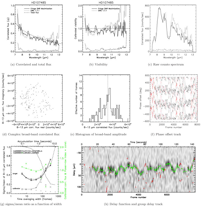
Figure 16: The same as Fig.15, but for the data taken on 2009-05-10.

Fig.16 shows a similar case to that shown in Fig.15, where the count rate is slightly lower and the coherence time is slightly shorter. The maximum S/N is thus slightly lower. However, the atmospheric conditions between target and calibrator observations seem to be well matched.

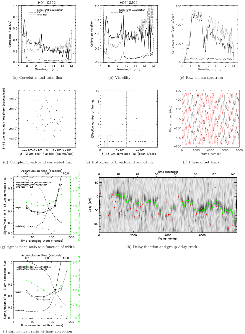
Figure 18: The same as Fig.17 but for another unresolved star HD110392 taken on 2009-05-09.

In Figs.17 and 18, we show the cases where there seems to be a difference in atmospheric conditions between target and calibrator fringe tracks. In these cases, we try to evaluate the difference by comparing the expected $\sigma/m$ curve for the target (triangles with dotted line in Fig.17(i) and 18(i)), as derived from the calibrator frames, with the observed curve for the target (squares with solid lines). We find that we can fit these two curves if we simply scale the time length of the calibrator frames (a factor of $\sim$0.7 in Fig.17(g), and $\sim$2.5 in Fig.18(g)). The scaling factor probably corresponds to the difference in the coherence time between target and calibrator frames. Therefore, we infer that we can obtain appropriate calibrations of the target frames if we use this time scaling factor. This correction also stabilizes the calibrated correlated flux over different $w$.

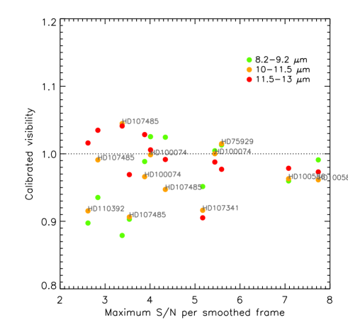
Figure 19: Comparison of deduced visibilities for sub-Jy calibrators.

Fig.19 shows the calibrated visibility of the 12 low and intermediate S/N observations of unresolved stars as a function of the maximum S/N per smoothed frame. We calculated the visibility in three different wavelength bins, avoiding the range affected by atmospheric ozone features. We confirm that the calibration procedure above correctly calibrates the data, although we see a slight tendency that, toward shorter wavelengths, the correlated flux is underestimated as the maximum S/N decreases. Based on the mean deviation and dispersion of these calibrated visibilities, we assign a systematic error in the correlated flux as 5% of the total flux, when the maximum S/N is at least larger than $\sim$2.5. Since the cases at lower S/N remain untested, we did not use the target datasets under this level in this paper.

A.5 Refinement of group delay determination

As described in section A.1, we use a large gsmooth parameter for faint targets to smooth over a large number of delay function frames and thus increase the S/N for delay determination and also strongly suppress the instrumental delay peaks. However, this also suppresses the atmospheric delay peaks at the time intervals where the delay is relatively quickly changing. As a result, the delay function image becomes quite ’blobby’, and strong delay peaks are left only where the atmospheric delay did not change rapidly.

To partially compensate for this effect, we implemented a simple iteration to determine the delay track. Namely, we first interpolated (over time) between the strong delay peaks to derive an approximate delay track. Then we used this approximate atmospheric delay track (plus instrumental delay) to rotate the original fringe spectra in the complex plane, and re-derived the delay function smoothed with the same gsmooth parameter. This makes the resulting delay peaks line up straighter over time, and thus recovers a larger number of frames with strong delay peaks. We cycled over this process a few times. For calibrator frames, this resulted in almost all the frames having strong peaks (i.e. even with the large gsmooth parameter). For target frames, significant fraction of frames is recovered, resulting in a good representation of the delay track even in a relatively low S/N case as shown in Fig.17.

In low S/N cases, we flagged frames that show delay peaks at positions that deviate significantly from the overall track obtained above. This was done by taking the histogram of the difference between the determined group delay track with that smoothed over many frames (typically $\sim$20-40 frames, set as 2 $\times$ gmoooth). The distribution can roughly be descibed by a Gaussian, and frames with large deviations ($>$ 10 $\sigma$) were excluded. In this rejection process, we did not select frames based on the strength of the delay peaks in order to avoid possible biasing.

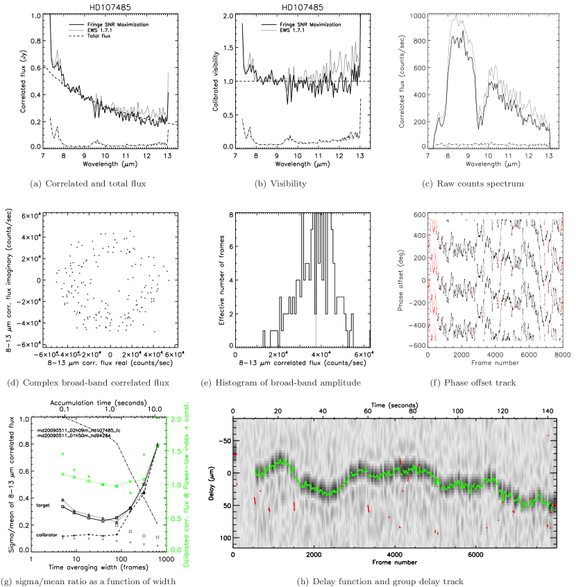
Figure 15: The results for the unresolved star HD107485 taken on 2009-05-11. ($a$) Our results for the calibrated correlated flux and its error are shown in solid and dot-dash line, respectively, while the correlated flux from a default reduction with EWS 1.7.1 (see text) is shown in dotted line. The dashed line is the total flux for this star which is obtained by scaling a template spectrum based on the known spectral type and IRAS flux. ($b$) The same as $a$ but deduced visibilities are shown instead of correlated flux. ($c$) The same as $a$ but raw counts spectra are shown. ($d$) Broad-band correlated flux measurements integrated over 7-13 $\mu$m (smoothed over a particular time width $w$) are shown on the complex plane. ($e$) Histogram of the amplitude of the broad-band correlated flux from the panel $d$ is shown. ($f$) The phase of the correlated flux as a function of frame number, i.e. time. The same track is repeatedly shown with 360$\degr$ offsets to clearly indicate the track as a function of time. The red points show excluded frames. ($g$) The ratio of the standard deviation $\sigma$ to mean $m$ of the correlated flux amplitude measurements is shown as a function of smoothing width $w$ in frames (lower axis) and in seconds (upper axis). The solid line with squares is for the target (HD107485) while the dashed line with plus signs is for the calibrator (see Table 9). The gray squares and gray plus signs (without any connecting lines) indicate the photon noise (see Sect.A.3) estimated for the target and calibrator, respectively. The dotted line with triangles shows the expected fractional dispersion $\sigma$/$m$ curve for the target, which is estimated from the $\sigma$/$m$ curve for the calibrator (i.e. the dahed line with plus signs) and the photon noise estimations (i.e. gray squares and plus signs with no connecting lines). The dash-dotted line indicates the relative correlated flux counts of the calibrator as a function of $w$, showing the relative effective system visibility at each $w$. The green circles show the relative calibrated broad-band correlated flux as a function of $w$. The green crosses show the relative power-law index of the calibrated correlated flux spectrum also as a function of $w$. ($h$) The delay function on the plane of delay versus frame number is drawn in gray scale image, showing the group delay track before the iteration described in Sect.A.5. The green and red points indicate non-rejected and rejected fringe peaks, respectively, after the iteration.

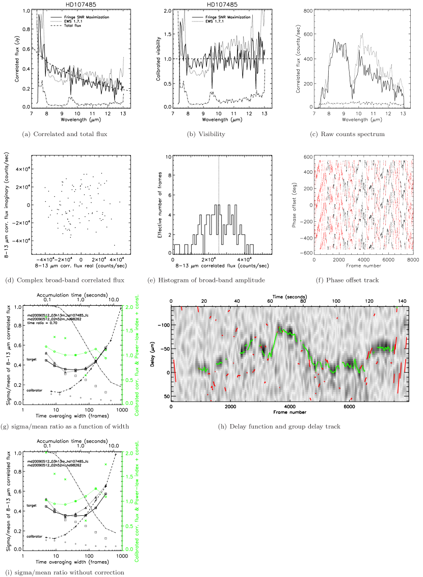
Figure 17: The same as Fig.15, but for the data taken on 2009-05-12. The panel ($g$) shows the $\sigma$/$m$ curve after the correction for the time scale difference between the target and calibrator, while the panel ($i$) shows the curves before the correction.

A.6 A note on total flux frames

For the targets observed with UTs that have total flux of less than a few Jy, it is better to implement an additional background subtraction using the sky regions very close to the target position. The residual of the primary background subtraction using chopped frames can still dominate the target flux for these relatively faint targets. An optional way to further reduce the systematic error from the background subtraction is to iteratively reject frames with the sky region counts having large deviations from the average. This was implemented in a small number of cases when the time fluctuation over the photmetry frames was significantly reduced after the frame rejection. With this additional sky subtraction, we averaged many sets of data, even from different nights, to obtain reliable total flux spectra, as confirmed with our VISIR photometry and spectrum.

Table 9: Observation log for sub-Jy unresolved stars.

name	flux	date & time		vis./flux	max
	(Jy)a	(UT)		calibrator	S/Nb
HD100586	0.82	2009-03-13	04:44	HD101666	7.1
		2009-03-15	04:00	HD101666	7.7
HD107341	0.75	2009-05-09	03:34	HD98262	5.2
HD75929	0.55	2009-03-15	01:02	HD100407	5.6
HD100074	0.45	2009-03-14	04:17	HD100407	5.4
		2009-03-15	02:19	HD100407	4.0
		2009-05-10	03:38	HD112213	3.9
HD107485	0.34	2009-05-10	01:14	HD94264	3.5
		2009-05-11	02:09	HD94264	4.3
		2009-05-12	03:06	HD98262	3.4
		2009-05-12	03:13	HD98262	2.8
HD110392	0.28	2009-05-09	02:15	HD94264	2.6

^a 12 $\mu$m Flux from IRAS Faint Source Catalog.
^b Maximum signal-to-noise ratio per smoothed frame for the correlated
flux integraged over the whole N-band.

Appendix B Mid-IR data plotted in conventional formats

In Fig 1 and 2 we show our flux and visibility data with normalizations using the inner radius $R_{\rm in}$. We show the same data in the mid-IR (after reddening corrections; see Sect.2.5) using conventional units in Fig 20 and 21, to facilitate direct comparisons with the data in the literature.

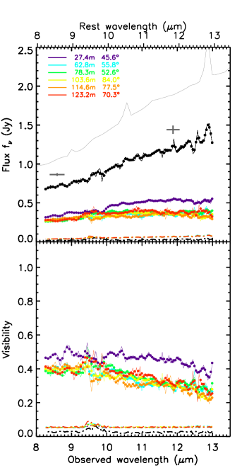
(a) NGC4151

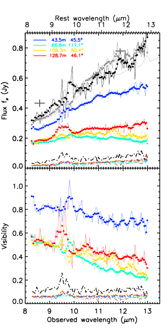
(b) NGC3783

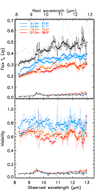
(c) ESO323-G77

Figure 20: All the mid-IR data shown in Figs 1 and 2 and summarized in Table 5 are plotted here in more conventional ways for (a) NGC4151, (b) NGC3783, and (c) ESO323-G77. Top: the total flux and correlated flux spectra taken with MIDI are shown in units of Jy. The filled circles indicate the spectra with a 5-pixel boxcar smoothing (3 pixel for NGC4151), while the spectra before the smoothing are shown with thin lines. The total flux is shown in black, while the correlated flux is shown in different colors for different baselines as indicated by the legend at top-left where the projected baseline lengths and PAs are written. The error spectra estimated for the smoothed spectra are shown at the bottom with dash-dot lines using the same corresponding colors. The two fluxes from the broad-band VISIR imaging are shown with error bars in thick gray lines. The thin gray spectra mostly at the highest flux levels are from the Spitzer IRS observations. The slightly darker gray spectrum shown for ESO323-G77 is from the VISIR spectroscopy. For NGC3783, the total flux taken in 2005 scaled to match the flux in 2009 (see Sect.2.1) is shown in gray color. Bottom: the resulting visibility spectra are shown using the same color scheme, with the error spectra excluding the total flux error contribution. The fractional total flux errors are drawn separately in black dash-dot lines.

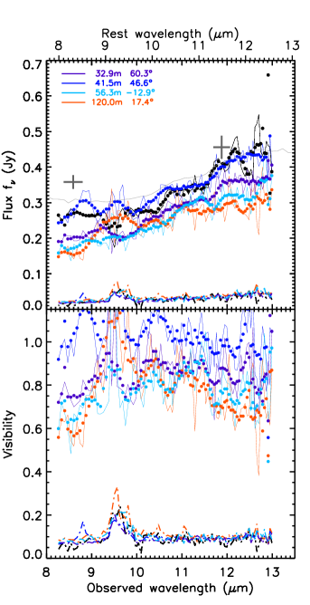
(a) H0557-385

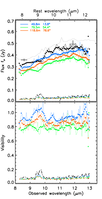
(b) IRAS09149

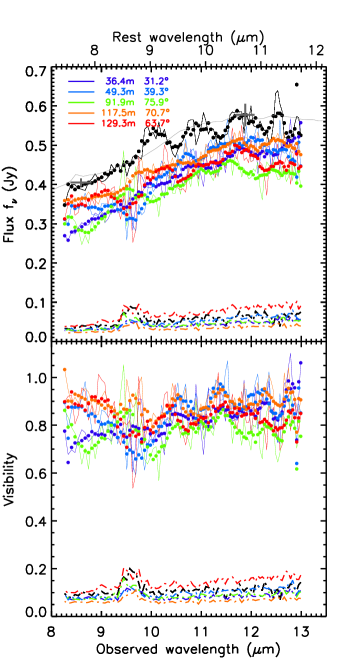
(c) IRAS13349

Figure 21: The same as Fig.20, but the data shown in solid lines are with the total flux smoothed by 3 pixels while those in filled circles are with total and correlated fluxes smoothed by 7 pixels. The figures are for (a) H0557-385, (b) IRAS09149-6206, and (c) IRAS13349+2438.

Appendix C Radial structure plot in linear scale

In Fig.3 we showed observed mid-IR visibilities of all the targets in a single plot to uniformly compare the radial structure of the objects in normalized units with spatial frequency in log scale. Here in Fig.22 we show exactly the same figure but with spatial frequency in linear scale, again to facilitate comparisons with the data in the literature.

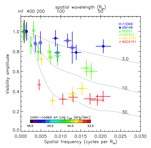
Figure 22: The same figure as Fig.3, but with the spatial frequency on a linear scale.