Ordinary Percolation with Discontinuous Transitions

Abstract

Percolation on a one-dimensional lattice and fractals such as the Sierpinski gasket is typically considered to be trivial because they percolate only at full bond density. By dressing up such lattices with small-world bonds, a novel percolation transition with explosive cluster growth can emerge at a nontrivial critical point. There, the usual order parameter, describing the probability of any node to be part of the largest cluster, jumps instantly to a finite value. Here, we provide a simple example of this transition in form of a small-world network consisting of a one-dimensional lattice combined with a hierarchy of long-range bonds that reveals many features of the transition in a mathematically rigorous manner.

Introduction

The percolation properties(Stauffer94, ) of networks are of significant interest — without percolation, any large-scale transport or communication through the network ceases. Much research has been dedicated to the understanding of percolation on randomly grown, complex networks(Barabasi03, ). Yet, the engineering of artificial networks with well-controlled features seems desirable. Indeed, there has been considerable interest in the properties of spatial networks, linking real-world geometry with small-world effects(Watts98, ; Boguna09, ; barthelemy_spatial_2010, ). In particular, networks possessing hierarchical features(Trusina04, ; Andrade05, ; Hinczewski06, ; SWPRL, ; Boguna09, ; PhysRevE.82.036106, ) relate to actual transport systems such as for air travel, routers, and social interactions. Certain hierarchical networks with a self-similar structure have been shown to exhibit novel features(Hinczewski06, ; Boettcher09c, ; Berker09, ; Nogawa09, ; Hasegawa10a, ; Boettcher10c, ). To these, we add here an unprecedented discontinuous transition in the formation of an extensive cluster for ordinary, random bond addition. Such an extensive cluster is said to percolate, as it contains a finite fraction of all nodes. Remarkably, this discontinuous transition can be derived exactly with recursive methods, as shown below.

For a random network that allows bonds between any pair of nodes, the possibility of a discontinuous (“explosive”) percolation transition has recently attracted considerable attention(Achlioptas09, ; ISI:000286751500010, ; ISI:000291093600009, ; ISI:000287844300028, ; PhysRevE.84.020101, ; ISI:000279888400004, ; FriedmanLandsberg09, ; RozenfeldGallosMakse09, ; RadicchiFortunato10, ; ChoKahngKim10, ; ISI:000277699600032, ; ISI:000288007800002, ; MannaChatterjee11, ). Such a transition raises the prospect that a minute increase in the bond-density $p$ of a network can suddenly make a large fraction of all nodes accessible, for instance, for the spreading of a contagion(Balcan09, ). Yet, all proposed mechanisms for such a transition require correlated bond additions(Achlioptas09, ). While further simulations of the dynamics of such correlated cluster formation(ISI:000279888400004, ; FriedmanLandsberg09, ; RozenfeldGallosMakse09, ; RadicchiFortunato10, ; ChoKahngKim10, ; ISI:000277699600032, ; ISI:000288007800002, ; MannaChatterjee11, ) seemed to support the existence of a discontinuity, evidence against it(ISI:000286751500010, ; ISI:000291093600009, ; ISI:000287844300028, ; PhysRevE.84.020101, ) finally mounted into a general proof of the impossibility of explosive percolation for any of the proposed mechanismsRiordan11 . In contrast to these efforts, we study ordinary (uncorrelated) bond additions but on networks with a recursive, hierarchical structure to induce such an explosive percolation dynamics. Understanding of explosive cluster formation will be significantly advanced when the discontinuity can be studied rigorously by simply adding bonds randomly to these networks.

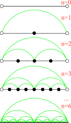
Figure 1: Recursive generation of a hierarchical network. (The network is displayed at full bond density, $p=1$.) In $(n=0)$-th generation, the network consists of a single bond between two end-nodes (open circles). The probability for an end-to-end path is obviously $T_{n=0}=p$. In successive generations $n+1=1,2,\ldots$, two sub-networks from the prior generation $n$ are merged together with the endpoints connected by a new long-range bond (shaded arcs). There is an end-to-end path with probability $T_{n+1}$, if either the new long-range bond exists (probability $p$, irrespective of $T_{n}$) or both prior sub-networks are present (probability $(1-p)\,T_{n}^{2}$), leading to Eq. (1). In each generation $n$ the network has $N=2^{n}+1$ nodes and $E=2^{n+1}-1$ bonds for an average degree $2E/N\sim 4$ for large $n$.

Results

Probability of a Spanning Cluster.

In our discussion we focus on a simple example of a hierarchical network that is developed in Fig. 1. In its hierarchical construction, networks from preceding generations are merged for successive generations for ever larger networks. The probability for an end-to-end path of the most elementary network at $n=0$, a single bond, is $T_{n=0}=p$. By merging two networks of generation $n$ side-by-side and adding a long-range bond to obtain a network of generation $n+1$, we recursively determine the probability $T_{n+1}$. This analysis is but one example of the real-space renormalization group (RG)(Plischke94, ).

The probabilities for an end-to-end path satisfy the recursion

$$T_{n+1} = p+(1-p)T_{n}^{2},\qquad\left(T_{0}=p\right),$$ (1)

as is explained in Fig. 1. In the limit of infinitely large networks we obtain for any $p$ the probability for such an end-to-end connection, $T^{*}(p)=\lim_{n\to\infty}T_{n}$, from the stationary solutions of Eq. (1), called fixed points. Setting $T_{n+1}\sim T_{n}\sim T^{*}$ in Eq. (1) yields a horizontal line of fixed points $T^{*}\equiv 1$ for all $p$, as well as arising line of fixed points,

$$T^{*}(p) = \frac{p}{1-p}\qquad\left(p\leq\frac{1}{2}\right).$$ (2)

Both lines intersect at $p=\frac{1}{2}$. Further analysis shows(Boettcher09c, ) that Eq. (2) is the stable solution for all $0<p<\frac{1}{2}$ that describes the actual behavior of large networks. I.e., very large networks possess an end-to-end connection with a finite probability approaching $0<T^{*}(p)<1$. However, for $\frac{1}{2}\leq p\leq 1$, the horizontal line is the only physical and stable solution such that a connection exists with certainty, $T^{*}=1$.

Origin of the Percolation Transition.

The phenomenology of percolation on hierarchical networks is quite distinct from that of lattices(Boettcher09c, ; Nogawa09, ; Berker09, ; Hasegawa10a, ). Specifically, on a lattice both, an end-to-end path and an extensive cluster, arise with certainty above the same critical bond density $p_{c}$. Each node attains a finite probability $P_{\infty}\left(p>p_{c}\right)>0$ to be connected to the spanning cluster. In contrast, hierarchical networks may have two transitions at a lower and an upper bond density, $p_{l}<p_{u}$. Below the lower transition $p_{l}$, all clusters remain finite and no end-to-end paths exists. Above the upper transition $p_{u}$, there is an extensive cluster and a certain end-to-end path, as on any lattice. But both transitions delimit an interval $p\in\left(p_{l},p_{u}\right)$ that contains fractal (sub-extensive) clusters with a finite probability $T^{*}$ for an end-to-end path, as given by Eq. (2). These clusters each harbor a vanishing fraction of all nodes, however, they diverge in size with $N^{\Psi}$, defining a new fractal exponent $0\leq\Psi\left(p\right)<1$(Nogawa09, ). Accordingly, the order parameter(Stauffer94, ; Plischke94, ) $P_{\infty}$ becomes non-zero only at $p_{u}$, making it the thermodynamically correct transition point, $p_{c}=p_{u}$. In the present network it is $p_{l}=0$ and $p_{u}=\frac{1}{2}$; more elaborate networks with exact but non-trivial $p_{l}$ and $p_{u}$ are discussed elsewhere(Boettcher09c, ).

We note that the simultaneous emergence of an extensive cluster with end-to-end paths appears to be special for “flat” geometries. Hierarchical networks posses what is called a hyperbolic geometry(PhysRevE.82.036106, ) for which most nodes are close to the periphery, similar to a tree, with many root-to-end paths. Correspondingly, parabolic networks would be very prone to clustering in the bulk with few paths to any peripheral node, i.e., an extensive cluster would emerge before paths that access the periphery arise.

Construction of the Order Parameter.

To reveal the nature of the transition, the probability $T^{*}(p)$ alone provides insufficient information. In addition, we have to derive the average size $\left\langle s_{\rm max}\right\rangle_{n}$ of the largest cluster and

$$P_{\infty}(p)=\lim_{n\to\infty}\frac{\left\langle s_{{\rm max}}\right\rangle_{n}}{N}$$ (3)

as the proper order parameter(Stauffer94, ) from cluster generating functions. Thus, we introduce two basic quantities: the probability $t_{i}^{(n)}(p)$ that both endnodes are connected to the same cluster of size $i$, and the probability $s_{i,j}^{(n)}(p)$ that the left endnode is connected to a cluster of size $i$ and the right endnote to a different cluster of size $j$. The corresponding generating functions to provide the average cluster size are defined as

$$T_{n}(x) = \sum_{i=0}^{\infty}t_{i}^{(n)}(p)x^{i},$$ (4)

$$S_{n}(x,y) = \sum_{i=0}^{\infty}\sum_{j=0}^{\infty}s_{i,j}^{(n)}(p)x^{i}y^{j}$$ (5)

and are depicted in Fig 2. $T_{n}(x)$ represents clusters with an effective bond between the endnodes while $S_{n}(x,y)$ represents those that fail to provide such a bond. The following manipulations, while subtle, only entail elementary manipulations that result in three coupled but linear recursions. Although we provide enough details here to reproduce the intermediate steps in a few lines, we have implemented those steps also as a Mathematica script provided in the Supplementary Software. Therein lies the advantage of our present example: The discontinuity can be obtained exactly and with ease.

The recursion relations for these generating functions are obtained in Fig. 3 by considering all possible configurations on three nodes, similar to Fig. 1 but now also taking cluster sizes into account. For each configuration, the type of effective bond between each of the nodes is checked, see Fig. 2, and these bonds are assigned a value $T_{n}(x)$ or $S_{n}(x,y)$, depending on the type of cluster each represents. As in Fig. 1, small world bonds are merely assigned the probability $p$ or $1-p$ for being present or not. Marking the increment in cluster size, the inner node provides a factor of $x$ or $y$ for its adjacent cluster, or unity if it remains isolated. The contribution of each configuration to the next generation is the product of the weights of the three bonds and of the intermediate node; all eight of these are determined in Fig. 3. From Fig. 3 we read off the recursions

$$T_{n+1}(x) = xT_{n}^{2}(x)+p\left[2xT_{n}(x)S_{n}(x,x)\right.$$ (6)

$$\left.+S_{n}(x,1)S_{n}(1,x)\right],$$

$$S_{n+1}(x,y) = (1-p)\left[xT_{n}(x)S_{n}(x,y)+\right.$$ (7)

$$\left.+yT_{n}(y)S_{n}(x,y)+S_{n}(x,1)S_{n}(1,y)\right],$$

initiated with $T_{0}(x)=p$, $S_{0}(x,y)=1-p$. Naturally, both equations reduce to Eq. (1) for $x=y=1$ where $T_{n}\left(1\right)=1-S_{n}\left(1,1\right)=T_{n}$.

The recursions in Eqs. (6,7) contain more information then is needed here and we simplify them in terms of functions of a single variable $x$. We define the functions $\Sigma_{n}(x)\equiv S_{n}\left(x,x\right)$ and ${\cal S}_{n}(x)\equiv S_{n}\left(x,1\right)=S_{n}\left(1,x\right)$ that, combined into a more efficient vector notation $\vec{V}=\left[T,\Sigma,{\cal S}\right]$, lead to

$$\vec{V}_{n+1}\left(x\right)=\vec{{\cal F}}\left(\vec{V}_{n}\left(x\right),x\right)$$ (8)

with a function-vector $\vec{{\cal F}}$ of non-linear components

$$\vec{{\cal F}}\left(\vec{V},x\right) = \left[\begin{array}[]{r}xT^{2}+2xpT\Sigma+p{\cal S}^{2}\\ (1-p)\left(2xT\Sigma+{\cal S}^{2}\right)\\ (1-p)\left(1+xT\right){\cal S}\end{array}\right].$$ (12)

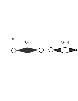
Figure 2: Diagramatic defintion of the generating functions. In the schematic for generating functions $T_{n}(x)$ and $S_{n}(x,y)$, the open circles represent the end-nodes, shaded areas indicate clusters that either span ($T_{n}$) or do not span ($S_{n}$) between the end-nodes. Clusters that do not reach an end-node are ignored.

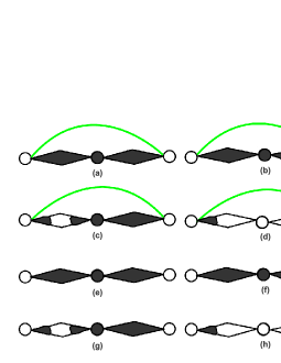
Figure 3: Diagramatic evaluation of the generating functions. All diagrams contributing to $T_{n+1}(x)$ or $S_{n+1}(x,y)$ in the $n$th RG step are shown. The remaining end-nodes (always-open circles) are not counted in the generating functions; the (black) connecting nodes increment the cluster size, accounted for by a factor of $x$ or $y$. The contribution of each configuration is: (a) $xpT_{n}^{2}(x)$, (b) $xpT_{n}(x)S_{n}(x,x)$, (c) $xpT_{n}(x)S_{n}(x,x)$, (d) $pS_{n}(x,1)S_{n}(1,x)$, (e) $x(1-p)T_{n}^{2}(x)$, (f) $x(1-p)T_{n}(x)S_{n}(x,y)$, (g) $y(1-p)T_{n}(y)S_{n}(x,y)$, and (h) $(1-p)S_{n}(x,1)S_{n}(1,y)$. As tallied up in Eqs. (6,7), configurations (a)-(e) span end-to-end and contribute to $T_{n+1}(x)$, while (f)-(h) do not span and contribute to $S_{n+1}(x,y)$.

As needed in Eq. (3), the mean size $\left\langle s_{{\rm max}}\right\rangle_{n}$ of the cluster connected to the endnodes results from the first moment of the generating functions. These are obtained via their first derivative in $x$ at $x=1$,

$$\left\langle s_{{\rm max}}\right\rangle_{n}=T_{n}^{\prime}\sim N^{\Psi\left(p\right)},$$ (13)

for a network of size $N=2^{n}+1\to\infty$.

Analysis of the Recursions for the Mean Cluster Size.

The mean size of the largest cluster, as needed in Eq. (3) to construct the order parameter, is obtained by Taylor-expanding Eq. (8) to first order in $\epsilon\equiv 1-x\to 0$. To zeroth order, each component in Eq. (8) evaluated at $x=1$ reproduces Eq. (1) again. To order $\epsilon$, we find an linear inhomogeneous recursion for $\vec{V}_{n}^{\prime}$, dropping the now-redundant argument $x=1$,

$$\vec{V}_{n+1}^{\prime} = \frac{\partial\vec{{\cal F}}}{\partial\vec{V}}\left(\vec{V}_{n}\right)\circ\vec{V}_{n}^{\prime}+\frac{\partial\vec{{\cal F}}}{\partial x}\left(\vec{V}_{n}\right)$$ (14)

with the Jacobian matrix

$$\frac{\partial\vec{{\cal F}}}{\partial\vec{V}}\left(\vec{V}\right)=\begin{bmatrix}2T+2p\Sigma,&2pT,&2p{\cal S}\\ 2(1-p)\Sigma,&2(1-p)T,&2(1-p){\cal S}\\ (1-p){\cal S},&0,&(1-p)\left(1+T\right)\end{bmatrix}$$ (15)

and the inhomogeneity from differentiating for $x$ explicitly

$$\frac{\partial\vec{{\cal F}}}{\partial x}\left(\vec{V}\right) = \left[\begin{array}[]{r}T^{2}+2pT\Sigma\\ 2(1-p)T\Sigma\\ (1-p)T{\cal S}\end{array}\right].$$ (19)

In Eqs. (15) and (19) we neglected the index $n$ on $\vec{V}$ and its components to simplify the presentation. They depend on $n$ through $\vec{V}_{n}=\left[T_{n},\Sigma_{n}=1-T_{n},{\cal S}_{n}=1-T_{n}\right]$. Since each network at $n=0$ only consists of endnodes, which are not counted, all clusters are initially empty, i.e., $\vec{V}_{0}^{\prime}=\left[0,0,0\right]$.

For large $n$ at $x=1$, i.e., near the fixed point $\vec{V}^{*}=\left[T^{*},\Sigma^{*}=1-T^{*},{\cal S}^{*}=1-T^{*}\right]$, it is easy to show that the inhomogeneity in Eq. (14) is subdominant, leaving a linear homogeneous system with constant coefficient-matrix $\frac{\partial\vec{{\cal F}}}{\partial\vec{V}}\left(\vec{V}^{*}\right)$. The largest eigenvalue $\lambda$ of this matrix provides the dominant contribution for each component of $\vec{V}_{n}^{\prime}$, i.e., $T_{n}^{\prime},\Sigma_{n}^{\prime},{\cal S}_{n}^{\prime}\sim\lambda^{n}$. We obtain $\lambda$ between the transitions, $0=p_{l}\leq p<p_{u}=\frac{1}{2}$, by applying Eq. (2) for $T^{*}$ in the matrix. Via Eq. (13) it is $\langle s_{{\rm max}}\rangle_{n}\sim\lambda^{n}$ for $n\to\infty$, which yields the fractal exponent

$$\Psi(p)=\frac{\ln\lambda}{\ln 2},\quad\lambda=\frac{1+3p-4p^{2}}{2(1-p)}+\sqrt{\frac{1-p(1-4p)^{2}}{4(1-p)}}.$$ (20)

The largest eigenvalue always remains $\lambda<2$ for $p<1/2$, i.e., $0\leq\Psi(p)<1$, which implies that the order parameter $P_{\infty}$ in Eq. (3) vanishes for $p<p_{u}$, hence, $p_{u}=p_{c}$.

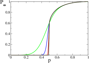
Figure 4: Plot of the order parameter $P_{\infty}\left(p\right)$ in Eq. (3). $P_{\infty}\left(p\right)$ is evaluated after $n=10^{k}$ iterations of the recursions in Eq. (14) with $k=1,\ldots,5$, displayed from left to right. This corresponds to system sizes of up to $N\approx 2^{n}\sim 10^{3010}$ nodes. It evolves slowly into a discontinuity at $p\to p_{c}=\frac{1}{2}$ with $P_{\infty}\left(p_{c}\right)=0.609793\ldots$. Convergence is slowest just below $p_{c}$, since finite-size corrections decay as $N^{\Psi\left(p\right)-1}$ with $1-\Psi\left(p\right)\sim 8\left(p_{c}-p\right)^{2}/\ln 2$ for $p\to p_{c}$ from Eq. (20).

Above and at the transition, $p_{c}\leq p\leq 1$, it is $T^{*}=1$ and Eq. (15) provides uniformly $\lambda=2$ as the largest eigenvalue (i.e., $\Psi\equiv 1$), indicating percolation in form of an extensive cluster. For a continuous transition, $P_{\infty}\left(p\right)\sim\left(p-p_{c}\right)^{\beta}\to 0$ with $\beta>0$ for $p\to p_{c}^{+}$. In contrast, Eq. (14) can be shown rigorously to provide a monotone increasing sequence for $T_{n}^{\prime}$, exactly at $p=p_{c}=\frac{1}{2}$ and for any $p$ above (see Supplementary Software). Therefore, the order parameter is positive definite even exactly at $p=p_{c}$, as displayed in Fig. 4. In fact, the continuity of $P_{\infty}\left(p\right)$ is interrupted merely because $T^{*}\equiv 1$ suddenly becomes an unstable fixed point of Eq. (1) below $p_{c}$. There, the stable branch transitions to Eq. (2) that lacks extensive clusters, $\Psi<1$. Hence, it is the intersection of two stable branches of fixed points $T^{*}$ at $p_{u}$ that causes a discontinuous transition. Such intersections of lines of fixed points is generic in hierarchical networks(Boettcher09c, ), whereas fixed points for percolation on lattices always remain isolated.

Discussion

We have shown that a hierarchy of small-world bonds grafted onto a one-dimensional lattice can result in an explosive percolation transition, even if bonds are added sequentially in an uncorrelated manner. The discontinuous transitions found in hierarchical networks are unique as alternative models based on correlated bond additions have been proven to failRiordan11 . At this point, the precise conditions to be imposed on the hierarchy of long-range bonds for obtaining this transition are not entirely clear. However, in each example we have obtained the addition of small-world bonds converted an initially finitely-ramified network into an infinitely ramified network to provide $p_{c}<1$, as several other networks demonstrate(Boettcher09c, ). In a finitely-ramified network, by definition(Stauffer94, ), the removal of just a finite number of bonds can separate off extensive clusters in the limit of large systems, $N\to\infty$, resulting in $p_{c}=1$. In contrast, studies of hierarchical systems with small-world bonds imposed on apriori infinitely-ramified 2d-lattices(Boettcher09c, ; Berker09, ; Hasegawa10a, ) appear to result in infinite-order transitions instead, which have been observed in many other networks(Dorogovtsev08, ).

Author contributions

S.B. and R.M.Z. developed the idea for this research, S.B. and V.S. worked out the formalism, and V.S. implemented the formalism, interpreted the results, and conducted numerical tests in close collaboration with S.B.

Competing Financial Interest Statement

None of the authors has any competing financial interests arising from any content in this paper.

References

- [1] D. Stauffer and A. Aharony. Introduction to Percolation Theory, Ed. CRC Press, Boca Raton, 1994.
- [2] Albert-Laszlo Barabasi. Linked: How Everything Is Connected to Everything Else and What It Means for Business, Science, and Everyday Life. Plume Books, April 2003.
- [3] D. J. Watts and S. H. Strogatz. Collective dynamics of ’small-world’ networks. Nature, 393:440–442, 1998.
- [4] M. Boguñá, D. Krioukov, and K. C. Claffy. Navigability of complex networks. Nature Physics, 5:74 – 80, 2009.
- [5] Marc Barthelemy. Spatial networks. Physics Reports, 499:1–101, October 2011.
- [6] Ala Trusina, Sergei Maslov, Petter Minnhagen, and Kim Sneppen. Hierarchy measures in complex networks. Phys. Rev. Lett., 92(17):178702, Apr 2004.
- [7] J. S. Andrade, H. J. Herrmann, R. F. S. Andrade, and L. R. da Silva. Apollonian networks: Simultaneously scale-free, small world, Euclidean, space filling, and with matching graphs. Phys. Rev. Lett., 94:018702, 2005.
- [8] M. Hinczewski and A. N. Berker. Inverted Berezinskii-Kosterlitz-Thouless singularity and high-temperature algebraic order in an ising model on a scale-free hierarchical-lattice small-world network. Phys. Rev. E, 73:066126, 2006.
- [9] S. Boettcher, B. Gonçalves, and H. Guclu. Hierarchical regular small-world networks. J. Phys. A: Math. Theor., 41:252001, 2008.
- [10] Dmitri Krioukov, Fragkiskos Papadopoulos, Maksim Kitsak, Amin Vahdat, and Marián Boguñá. Hyperbolic geometry of complex networks. Phys. Rev. E, 82(3):036106, Sep 2010.
- [11] S. Boettcher, J. L. Cook, and R. M. Ziff. Patchy percolation on a hierarchical network with small-world bonds. Phys. Rev. E, 80:041115, 2009.
- [12] A. Nihat Berker, Michael Hinczewski, and Roland R. Netz. Critical percolation phase and thermal Berezinskii-Kosterlitz-Thouless transition in a scale-free network with short-range and long-range random bonds. Phys. Rev. E, 80(4):041118, Oct 2009.
- [13] Tomoaki Nogawa and Takehisa Hasegawa. Monte Carlo simulation study of the two-stage percolation transition in enhanced binary trees. J. Phys. A: Math. Theor., 42(14):145001, 2009.
- [14] Takehisa Hasegawa, Masataka Sato, and Koji Nemoto. Generating-function approach for bond percolation in hierarchical networks. Phys. Rev. E, 82(4):046101, Oct 2010.
- [15] S. Boettcher and C. T. Brunson. Fixed point properties of the Ising ferromagnet on the Hanoi networks. Phys. Rev. E, 83:021103, 2011.
- [16] Dimitris Achlioptas, Raissa M. D’Souza, and Joel Spencer. Explosive percolation in random networks. Science, 323(5920):1453–1455, 2009.
- [17] R. A. da Costa, S. N. Dorogovtsev, A. V. Goltsev, and J. F. F. Mendes. Explosive Percolation Transition is Actually Continuous. Phys. Rev. Lett., 105:255701, 2010.
- [18] Peter Grassberger, Claire Christensen, Golnoosh Bizhani, Seung-Woo Son, and Maya Paczuski. Explosive Percolation is Continuous, but with Unusual Finite Size Behavior. Phys. Rev. Lett., 106:225701, 2011.
- [19] Jan Nagler, Anna Levina, and Marc Timme. Impact of single links in competitive percolation. Nature Physics, 7(3):265–270, MAR 2011.
- [20] Hyun Keun Lee, Beom Jun Kim, and Hyunggyu Park. Continuity of the explosive percolation transition. Phys. Rev. E, 84:020101, Aug 2011.
- [21] N. A. M. Araujo and H. J. Herrmann. Explosive Percolation via Control of the Largest Cluster. Phys. Rev. Lett., 105:035701, 2010.
- [22] Eric J. Friedman and Adam S. Landsberg. Construction and analysis of random networks with explosive percolation. Phys. Rev. Lett., 103(25):255701, 2009.
- [23] Hernán D. Rozenfeld, Lazaros K. Gallos, and Hernán A. Makse. Explosive percolation in the human protein homology network. Eur. Phys. J. B, 75(3):305–310, 2010.
- [24] Filippo Radicchi and Santo Fortunato. Explosive percolation: a numerical analysis. Phys. Rev. E, 81(3):036110, 2010.
- [25] Y. S. Cho, B. Kahng, and D. Kim. Cluster aggregation model for discontinuous percolation transition. Phys. Rev. E, 81:030103(R), 2010.
- [26] Raissa M. D’Souza and Michael Mitzenmacher. Local Cluster Aggregation Models of Explosive Percolation. Phys. Rev. Lett., 104(19), MAY 14 2010.
- [27] Nuno A. M. Araujo, Jose S. Andrade, Jr., Robert M. Ziff, and Hans J. Herrmann. Tricritical Point in Explosive Percolation. Phys. Rev. Lett., 106:095703, 2011.
- [28] S. S. Manna and A. Chatterjee. A new route to explosive percolation. Physica A, 390(2):177 – 182, 2011.
- [29] D. Balcan, V. Colizza, B. Goncalves, H. Hu, J. J. Ramasco, and A. Vespignani. Multiscale mobility networks and the spatial spreading of infectious diseases. Proc. Natl. Acad. Sci., 106:21484–21489, 2009.
- [30] Oliver Riordan and Lutz Warnke. Explosive percolation is continuous. Science, 333(6040):322–324, 2011.
- [31] M. Plischke and B. Bergersen. Equilibrium Statistical Physics, 2nd edition. World Scientifc, Singapore, 1994.
- [32] S. N. Dorogovtsev, A. V. Goltsev, and J. F. F. Mendes. Critical phenomena in complex networks. Rev. Mod. Phys., 80:1275–1335, 2008.