Electronic excitations and electron-phonon coupling in bulk graphite through Raman scattering in high magnetic fields

Abstract

We use polarized magneto-Raman scattering to study purely electronic excitations and the electron-phonon coupling in bulk graphite. At a temperature of 4.2 K and in magnetic fields up to 28 T we observe $K$-point electronic excitations involving Landau bands with $\Delta|n|=0$ and with $\Delta|n|=\pm 2$ that can be selected by controlling the angular momentum of the excitation laser and of the scattered light. The magneto-phonon effect involving the $E_{2g}$ optical phonon and $K$-point inter Landau bands electronic excitations with $\Delta|n|=\pm 1$ is revealed and analyzed within a model taking into account the full $k_{z}$ dispersion. These polarization resolved results are explained in the frame of the Slonczewski-Weiss-McClure (SWM) model which directly allows to quantify the electron-hole asymmetry.

I Introduction

Magneto-optical spectroscopy has been used to study the graphene/graphite structures for long time, but mostly transmission/reflectivity type of experiments (essentially in far-infrared spectral range) have been explored so far Galt et al. (1956); Schroeder et al. (1968); Toy et al. (1977); Li et al. (2006); Sadowski et al. (2006); Jiang et al. (2007); Orlita et al. (2008a, b); Henriksen et al. (2007); Orlita et al. (2009); Chuang et al. (2009); Orlita and Potemski (2010). Relevant for these systems, low energy electronic excitations can be optionally probed with Raman scattering methods Faugeras et al. (2011). These methods have been widely used to investigate phonon resonances in different carbon materials Dresselhaus et al. (2010), but advantages of combining them with application of magnetic fields have been recognized only recently Ando (2007a); Goerbig et al. (2007); Kashuba and Fal’ko (2009); Mucha-Kruczynski et al. (2010).

Indeed, magneto-Raman scattering experiments provide a spectacular demonstration of hybridization between optical phonon and electronic excitations in epitaxial graphene Faugeras et al. (2009) and graphene locations on graphite surface Yan et al. (2010); Faugeras et al. (2011). What is perhaps even more important is that such experiments allow also to probe purely electronic excitations in these systems Faugeras et al. (2011). When a magnetic field is applied across the layer, the electronic bands condense into Landau levels whose characteristic energy ladders (fan charts) reflect the specific dispersion relation of electronic states in the absence of the magnetic field. Magneto-Raman scattering can be used to trace selected inter Landau level excitations. This method, with all its advantages of a visible optics technique (spatial focusing, polarization resolved measurements), appears now as a valuable option for Landau level spectroscopy to study other sp²-bonded carbon allotropes, such as bulk graphite, investigated in this work.

In spite of recent efforts Garcia-Flores et al. (2009), the magneto-Raman scattering response of bulk graphite has not been so far clearly identified in experiments. Theoretical studies addressing this specific problem seem to be also missing. Relevant for our results are, however, predictions for a bilayer graphene Mucha-Kruczynski et al. (2010) which is the basic unit in construction the Bernal-stacking of graphite.

As a layered material, graphite is strongly anisotropic but still represents a three dimensional electronic system. In this respect, graphite is very different from its layer-components: purely two-dimensional monolayer or bilayer graphene. Electrons can easily move within the graphitic layers, but electronic states also remain dispersive in the direction across the layers. When a magnetic field is applied across the layers, we deal with Landau bands in graphite in contrast to discrete Landau levels in purely 2D systems (monolayer or bilayer graphene). Band structure of graphite is commonly described using the SWM model Slonczewski and Weiss (1958); McClure (1956). There is a general consensus on the validity of this tight binding approach. However, it implies up to seven hoping-integral parameters and the exact values of some of them remain controversial and this is despite very long history of the research on graphite.

Our magneto-Raman scattering experiments on graphite reveal a series of features which we attribute to electronic excitations between Landau bands in this material. The magnetic field evolution of the E_2g phonon excitation is also investigated. The observed electronic and phonon excitations are shown to follow the characteristic selection rules defined by the appropriate transfer of angular momentum between the incoming and outgoing, circularly-polarized photons. Polarization-resolved experiments together with appropriate modelling of electronic bands allow us to conclude about the relevant electron-hole asymmetry of the graphitic bands. Although our experiments are mostly sensitive to electronic states in the vicinity of the particular K-point of the graphite Brillouin zone, the three dimensional nature of this material is clearly reflected in the spectral shape of the observed electronic excitations and in the character of the investigated magneto-phonon resonances. Notably the E_2g phonon of graphite is shown to hybridize with a quasi-continuous spectrum of inter Landau band excitations, in contrast to similar effect in graphene involving the discrete LL transitions.

The paper is organized as follows: section II describes the experimental set-up, while the electronic properties of bulk graphite and the Raman scattering selection rules are presented in section III. Experimental results obtained in the co- and crossed-circular polarization configuration are presented in section IV, together with the magneto phonon effect of bulk graphite and experiments performed at room temperature. We finally present our conclusions.

II Experiment

The polarized Raman scattering response of bulk graphite at low temperature and in high magnetic fields, was measured with a home made confocal micro-Raman scattering set-up. A monolithic miniaturized optical table, made of titanium, has been designed to operate in a helium exchange gas at T$=4.2$K and in high magnetic field environments. A mono-mode optical fiber with $5\,\mu\mbox{m}$ core was used to bring the $\lambda=784\,\mbox{nm}$ excitation from a Ti:Saphire laser to the sample. The excitation beam is focused with lenses down to $\sim 1\,\mu\mbox{m}$ spot. Scattered light is then collected by a multi-mode $200\,\mu\mbox{m}$ optical fiber before being analyzed by a $500$ mm spectrometer equipped with a diffraction grating and a nitrogen cooled CCD. Our miniaturized optical table can host different optical filters that are used at liquid helium temperature and in high magnetic fields. Band-pass filters (laser line and notch filters) are used first to clean the laser coming out of the mono-mode fiber and to filter the elastically scattered laser before the collection optical fiber. They impose a cut-off energy of $\sim 350\,\mbox{cm}^{-1}$ from the laser line. A set of quarter wave plates and linear polarizers, placed close to the sample, are then used to circularly polarize the excitation beam and the collected signal to achieve both co- and crossed-circular polarization configurations. The two different co-circular ($\sigma^{-}/\sigma^{-}$ and $\sigma^{+}/\sigma^{+}$) or cross-circular ($\sigma^{-}/\sigma^{+}$ and $\sigma^{+}/\sigma^{-}$) configurations were obtained by changing the direction of the magnetic field with respect to the light propagation direction. Optical power on the sample was fixed to $5\,\mbox{mW}$. The sample is mounted on a set of translation piezzo stages which allow to move the sample under the laser spot with a sub-micrometer resolution.

The surface of natural graphite is known to be inhomogeneous and graphene flakes decoupled from the surface can be found. They have been evidenced by low temperature STM experiments Li et al. (2009a), studied by an EPR-like technique in magnetic fields Neugebauer et al. (2009) and mapped with micro-Raman scattering measurements in high magnetic fields revealing their graphene-like electronic excitation spectrum Faugeras et al. (2011) and the associated magneto-phonon effect Yan et al. (2010); Faugeras et al. (2011). To unravel the electronic properties of bulk graphite, we place the laser spot outside of these decoupled graphene flakes and measure the magnetic field evolution of the Raman scattering spectrum. Similar results were obtained using two different sources of natural graphite and Highly Oriented Pyrolitic Graphite (HOPG) and in the following, we will only discuss the case of natural graphite which shows, in our experiment, a slightly higher signal level.

III Theoretical outline

III.1 Graphite band structure

A conventional description of the band structure of bulk graphite and its evolution with the magnetic field relies on the SWM model with its seven $\gamma_{0},\ldots,\gamma_{5},\Delta$ tight binding parameters Slonczewski and Weiss (1958); McClure (1956); Nakao (1976). This model has been used to describe most of previous data obtained from magneto-transport Soule (1958); Soule et al. (1964); Woollam (1970); Schneider et al. (2009), infrared magneto-reflectivity Schroeder et al. (1968); Toy et al. (1977); Li et al. (2006), and magneto-transmission Orlita et al. (2008b, 2009); Chuang et al. (2009) experiments. It predicts the existence of massive carriers near the $K$ point with a parabolic in-plane dispersion and of massless carriers near the $H$ point with a linear in-plane dispersion. The Fermi energy is $\sim 15\,\mbox{meV}$ and, under an applied magnetic field, Landau bands are formed with a continuous dispersion along $k_{z}$, from equally spaced and linear in $B$ Landau levels at the $K$ point to non-equally spaced and $\sqrt{B}$ evolving Landau levels at the $H$ point Nakao (1976). Even though there is still no consensus concerning the precise values of the SWM parameters, mainly because of the different energy ranges probed in different experiments and because of the lack of polarization resolved measurements that would reveal unambiguously the effect of electron-hole asymmetry, the validity of the SWM model is generally accepted.

The evolution in magnetic field of electronic levels in bulk graphite has been calculated following the approach of Nakao Nakao (1976) and Landau levels are labelled following the bilayer graphene convention Abergel and Fal ko (2007) as sketched in Fig. 1. The infinite order magnetic field Hamiltonian was reduced to a $600\times 600$ matrix before the diagonalization procedure. Electronic excitations are labelled as $L_{n,n^{\prime}}$ where $n$ and $n^{\prime}$ are the indices of the Landau levels involved in the excitation $n\to{n}^{\prime}$.

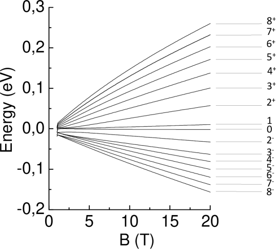
Figure 1: Evolution of the Landau levels at the K point of the graphite first Brillouin zone calculated within the SWM model and Landau levels’ indices.

Instead of the full SWM model, it is often sufficient to use the effective two-parameter model, which gives parabolic dispersion in the plane with the slope of the parabolas depending on $k_{z}$, the wave vector measured in the units of the inverse inter-layer spacing ($k_{z}=0$ at the $K$ point, and $k_{z}=\pi/2$ at the $H$ point). This model is obtained by (i) neglecting all SWM parameters except two, $\gamma_{0}$ and $\gamma_{1}$, the intralayer and the interlayer nearest-neighbor hopping integrals, respectively, and (ii) projecting the resulting $k_{z}$-dependent $4\times{4}$ Hamiltonian on the two low-energy bands. At each value of $k_{z}$, the Hamiltonian is identical to that of a graphene bilayer determined by the effective parameters $\gamma_{0}$ and $\gamma_{1}^{*}=2\gamma_{1}\cos k_{z}$. Since at the $K$ point $k_{z}=0$, the corresponding $\gamma_{1}^{*}$ is twice enhanced with respect to $\gamma_{1}$ describing the real graphene bilayer Partoens and Peeters (2007); Koshino and Ando (2008). This effective two-parameter parabolic model has proven to bring a fair frame to describe magneto-optical experiments Orlita et al. (2009); Chuang et al. (2009).

Still, the effective two-parameter parabolic model misses several effects, such as the in-plane trigonal warping, described by the $\gamma_{3}$ parameter of the full SWM model, as well as the electron-hole asymmetry. The latter is contributed by all remaining parameters ($\gamma_{2},\gamma_{4},\gamma_{5},\Delta$). To simplify the analysis, one can notice that at $k_{z}=0$, the $\gamma_{2},\gamma_{5},\Delta$ do not enter independently; eigenstates and transition energies depend only on their combination $\Delta_{eff}\equiv\Delta+2\gamma_{5}-2\gamma_{2}$, as can be seen from Eqs. (9), (10) of the Appendix. This combination determines the asymmetry in the positions of the split-off bands exactly at the $K$ point. For non-zero values of the in-plane wave vector, the electron-hole asymmetry is determined by both $\gamma_{4}$ and $\Delta_{eff}$, and it is not easy to separate the effects of the two. Throughout the paper, we use a set of SWM parameters derived from our polarization-resolved magneto-Raman scattering experiments. We will detail in the following sections how these parameters are determined, essentially from the crossed circular polarization configuration measurements which allow to directly quantify the electron-hole asymmetry.

III.2 Selection rules for Raman scattering

Generally, the Raman scattering selection rules for graphite can be deduced from its symmetry group, $D_{6h}$. However, the low-energy electronic Hamiltonian, as derived from the SWM model, is dominated by terms which have a higher symmetry. As a consequence, the electronic dispersion is almost isotropic with respect to continuous rotations of electronic momentum around the $H-K-H$ line. This isotropy is broken only by the trigonal warping term, governed by the $\gamma_{3}$ parameter of the SWM model. This term restricts the symmetry to the momentum rotations by $\pm{2}\pi/3$. As a result, the quantum number $m_{z}$, associated with the rotational symmetry (angular momentum), which could assume all integer values from $-\infty$ to $\infty$ in the case of the continuous rotational symmetry, has only three distinct values for the three-fold symmetry: all $m_{z}$’s differing by a multiple of 3, become equivalent. However, since the trigonal warping is small at energies, relevant for the present work, all transitions which are allowed by $D_{6h}$, can be further classified into strongly allowed (those which are allowed even when $\gamma_{3}=0$, thus surviving the continuous rotational symmetry), and weakly allowed (those which require a non-zero trigonal warping). The wording ”strongly” and ”weakly” allowed does not, however, refer to the apparent intensity of the excitation.

An example of a weakly allowed process is the Raman process responsible for the $G$ band feature. Indeed, trigonal warping is necessary for the appearance of the $G$ band feature, as was shown for monolayer graphene in Refs. Basko, 2008, 2009; in bilayer graphene and graphite the situation is analogous. The reason is that the circularly polarized photons carry an angular momentum $m_{z}=\pm{1}$, and out of two degenerate phonon modes, one can also choose two linear combinations carrying angular momentum $m_{z}=\pm{1}$. Then if a $\sigma^{+}$ photon ($m_{z}=-1$) is absorbed by the sample, the only way to conserve angular momentum is to emit a $\sigma^{-}$ photon ($m_{z}=+1$) and a phonon with $m_{z}=+1$. Then the total change in the angular momentum is $+3$, which is equivalent to 0, thanks to trigonal warping. Thus, the $G$ band feature is observed in the cross-circular polarization configuration.

An inter-Landau-level excitation $n^{-}\to(n+m_{z})^{+}$ carries an angular momentum $m_{z}$. This immediately designates the transitions with $\Delta|n|=0$ and $\Delta|n|=\pm{2}$ as the strongly allowed processes in the co-circular and cross-circular polarization configurations, respectively. As in the case of a graphene monolayer, the strongly allowed coupling for the magneto-phonon effect in a graphene bilayer Ando (2007b) involves the optical phonon and electronic excitations with $\Delta|n|=\pm 1$ (optical-like excitations). These optical-like excitations are not expected to be Raman active without trigonal warping. Nevertheless, if $\gamma_{3}$ is included then the trigonal warping is expected to weakly allow these excitations. For instance, an excitation $L_{n^{-},(n+1)^{+}}$ with $\Delta|n|=+1$ can be observed in Raman scattering experiments, because of the trigonal warping induced mixing of the levels $n^{-}$ and $(n+3)^{-}$, through the excitation $L_{(n+3)^{-},(n+1)^{+}}$ which is strongly allowed in Raman scattering. Interesting is the fact that $\Delta|n|=\pm 1$ are expected to be observed in the same crossed circular polarization as $\Delta|n|=\mp 2$ excitations. A signature of such transitions has indeed been seen in the present experiment.

IV Experimental results and discussion

IV.1 Co-circular configuration

Fig. 2(a) shows representative Raman scattering spectra in the co-circular polarization configuration, with the $B=0$ spectrum subtracted. In this configuration, the $G$ band feature is absent, as discussed in Sec. III.2. Starting from $B\sim{}2\,\mbox{T}$, many magnetic field dependent features are observed, with energies increasing with the magnetic field. The observed line shape is strongly asymmetric with a long tail at high energies due the fact that the states involved in the scattering process do not belong to discrete Landau levels, but to Landau bands with a dispersion along $k_{z}$. The width of these features, about $50\,\mbox{cm}^{-1}$, is mostly determined by this $k_{z}$ dispersion, rather by any scattering mechanism. To gain more quantitative understanding of the line shape, we note that the Raman matrix element does not depend on the energy of the electronic states involvedMucha-Kruczynski et al. (2010), so the scattered intensity $I(\omega)$ is simply proportional to the joint density of states for excitations between Landau levels $n^{-}$ and $n^{+}$:

$$I_{B}(\omega)\propto\frac{1}{l_{B}^{2}}\int\limits_{0}^{\pi/2}dk_{z}\sum_{n\geq{2}}\delta\left(\omega-\epsilon_{n^{+}}+\epsilon_{n^{-}}\right),$$ (1)

where $\epsilon_{n^{\pm}}$ are the Landau level energies, and the magnetic length, $l_{B}=(eB/c)^{-1/2}$, keeps track of the Landau level degeneracy. In the two-parameter parabolic model, the Landau level energies are given by

$$\epsilon_{n^{\pm}}=\pm\sqrt{n(n-1)}\,\frac{\Omega_{B}}{\cos{k}_{z}},\quad\Omega_{B}=\frac{\gamma_{0}^{2}}{\gamma_{1}}\left(\frac{3a}{2l_{B}}\right)^{2},$$ (2)

where $a$ is the in-plane distance between neighboring carbon atoms. For $\epsilon_{n^{\pm}}$ given by Eq. (2), Eq. (1) gives

$$\frac{I_{B}(\omega)}{I_{B=0}}=2\Omega_{B}\sum_{n\geq{2}}\frac{\omega_{n}/\omega}{\sqrt{\omega^{2}-\omega_{n}^{2}}},$$ (3)

where $\omega_{n}\equiv\left.\epsilon_{n^{+}}-\epsilon_{n^{-}}\right|_{k_{z}=0}$. This expression describes well the tail on the high-frequency side of each peak, and has a square-root-type singularity at $\omega\to\omega_{n}$. The singularity can be cut off by replacing the $\delta$-function in Eq. (1) by a Lorentzian with full width at half-maximum $\Gamma$. This results in a somewhat more complicated, but still explicit analytical expression for the Raman spectrum:

$$\frac{I_{B}(\omega)}{I_{B=0}}=\sum_{n\geq{2}}\frac{2\Omega_{B}}{\omega_{n}}\mathop{\mathrm{Im}}\nolimits{f}\!\left(\frac{\omega-i\Gamma}{\omega_{n}}\right),$$ (4)

$$f(x)=\frac{1}{2x}+\frac{2/\pi}{x\sqrt{x^{2}-1}}\,\mathop{\mathrm{arctanh}}\nolimits\sqrt{\frac{x+1}{x-1}}.$$ (5)

In fact, the simple expression (2) does not reproduce well the peak positions; the full SWM model taking into account the electron-hole asymmetry is needed for this, as will be discussed below. Still, if we take Eqs. (4), (5) and substitute for $\omega_{n}$ the actual peak positions, the resulting expression describes the spectrum remarkably well, as shown in Fig. 2(b) for two values of the magnetic field. We have taken $\Gamma=14\,\mbox{cm}^{-1}$ for $B=12\,\mbox{T}$ and $\Gamma=20\,\mbox{cm}^{-1}$ for $B=20\,\mbox{T}$. The discrepancy between Eq. (4) and the experimental spectrum around the minima between the peaks can be improved by taking the full SWM result for $\epsilon_{n^{\pm}}$.

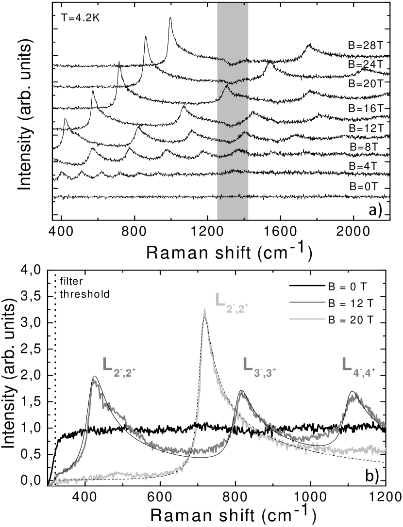
Figure 2: a) Representative Raman scattering spectra with subtracted $B=0$ T spectrum in the $\sigma^{-}/\sigma^{-}$ configuration showing many asymmetric magnetic field dependent features. Spectra are shifted for clarity. The gray region indicates an energy range where a magnetic field dependent background feature affects the normalized spectra. b) Raw Raman scattering spectra to compare, at 3 different values of the magnetic field, the scattered intensity. Solid and dashed lines are calculated within the two-parameter parabolic model (see main text for details). The vertical dotted line represents the cut-off energy of the optical edge-filter used to remove the laser line.

Fig. 2(b) shows that there exist an electronic contribution to the $B=0$ Raman scattering spectrum of bulk graphite, which is flat as a function of energy (between $300$ and $1200$ cm^-1), but that can be identified by applying a magnetic field. With the three Raman scattering spectra presented in this figure, one can directly compare the amplitude of the scattered light. When a magnetic field is applied, the energy independent response from low energy electronic excitations transforms into discrete features due to Landau quantization and one can identify the ”apparent background” signal in this experiment with the scattered amplitude at energies lower than the $L_{2^{-},2^{+}}$ excitation, which is set to zero in Fig. 2(b). In this particular experiment, we use magnetic field to change the electronic excitation spectrum, but one could expect a similar trend for gated graphene flakes. Changing the gate voltage would result in a continuous change of the $2E_{F}$ threshold in analogy to the tuning of the absorption threshold as a function of the Fermi energy observed in infrared absorption experiments Li et al. (2009b). One may also notice that the amplitude of the scattered light between any two given peaks L${}_{n^{-},n^{+}}$ and L${}_{(n+1)^{-},(n+1)^{+}}$ does not depend on the magnetic field. This can be seen directly from Eq. (1), which does not rely on approximation (2): as long as Landau level energies are proportional to $B$ (which is the case for $\omega<1000\,\mbox{cm}^{-1}$), the magnetic field drops out of $I_{B}(\omega_{n+1})$.

Table 1: SWM parameters used for the calculations

SWM parameter	full model (eV)	parabolic model (eV)
$\gamma_{0}$	3.08	3.15
$\gamma_{1}$	0.38	0.38 ($=\frac{\gamma_{1}^{*}}{2}$)
$\gamma_{3}$	0.315	0
$\gamma_{4}$	0.044	0
$\Delta+2\gamma_{5}-2\gamma_{2}$	0.22	0

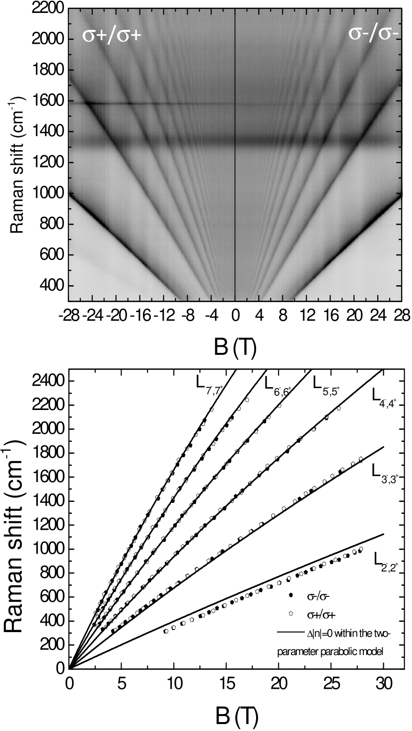
Figure 3: Upper panel: False color map of the scattered intensity at $T=4.2$ K as a function of the magnetic field in the two co-circular configurations (raw data). Lower panel: Position of the maxima of scattered light as a function of the magnetic field in the $\sigma^{+}/\sigma^{+}$ (black dots) and $\sigma^{-}/\sigma^{-}$ (open dots) configurations. Solid black lines are the $\Delta|n|=0$ electronic excitations calculated within the two-parameter parabolic model using the parameters described in Table. I.

The upper panel of Fig. 3 shows a false color map of the scattered intensity as a function of the magnetic field for the two $\sigma^{-}/\sigma^{-}$ and $\sigma^{+}/\sigma^{+}$ configurations. The evolution of these features is nearly linear with the magnetic field which is expected for carriers with a parabolic dispersion. The evolution of the maxima of the scattered light intensity as a function of the magnetic field is presented in the lower panel of Fig. 3 for the $\sigma^{-}/\sigma^{-}$ (open dots) and $\sigma^{+}/\sigma^{+}$ (black dots) configurations. We present in this figure the results of the corresponding excitations calculated within the two-parameter parabolic model with $\gamma_{0}=3.15$ eV, $\gamma_{1}^{*}=0.760$ eV (black lines). In a first approximation, this model allows to describe well the overall behavior of excitations involving Landau levels with $n>2$. The clear limitations of this model appear at low energies with the $L_{2^{-},2^{+}}$ excitation which is overestimated, mainly because of the missing $\gamma_{3}$ parameter relevant at low energies.

IV.2 Crossed circular configuration

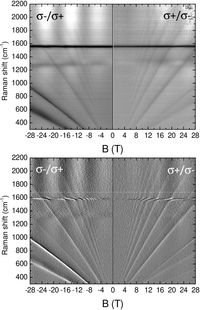
Figure 4: Upper panel: False color map of the scattered intensity at T=4.2K as a function of the magnetic field in the two crossed circular configurations. Lower panel: Derivative of the scattered light intensity as a function of the magnetic field.

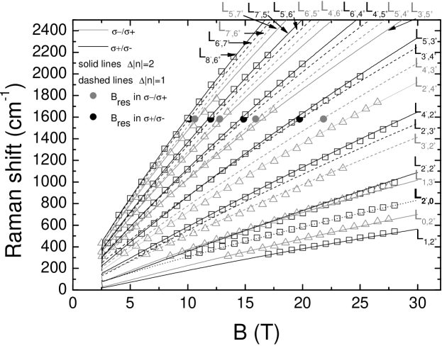
Figure 5: Maxima of scattered intensity as a function of the magnetic field for $\sigma^{-}/\sigma^{+}$ (gray open triangles) and $\sigma^{+}/\sigma^{-}$ (black open squares), together with $\Delta|n|=\pm 2$ electronic excitations calculated using the parameters presented in Table. I within the two-parameter parabolic model (black and gray solid lines) and $\Delta|n|=\pm 1$ electronic excitations (black and gray dashed lines). The gray and black circles correspond to the phonon resonances observed in $\sigma^{+}/\sigma^{-}$ and $\sigma^{-}/\sigma^{+}$ configurations respectively. The line $L_{2^{-},0}$ is calculated at $k_{z}$=0.3.

The crossed circular polarization configuration is expected to select excitations of the $E_{2g}$ symmetry which includes the optical phonon ($G$ band feature) and electronic excitations involving hole and electron states with $\Delta|n|=\pm 2$ (Ref. Kashuba and Fal’ko, 2009), which correspond to angular momentum $m_{z}=\pm 2$. We present in the upper panel of Fig. 4 a false-color map of the scattered intensity as a function of the magnetic field for both crossed circular polarization configuration and, in the lower panel of the same figure, a false color map of the derivative with respect to the magnetic field ($\Delta B=0.32$ T and spectra acquired every 0.08 T) of the same data. In these figures, many magnetic field dependent features can be observed, as well as a pronounced oscillatory behavior of the G-band feature that will be discussed in detail in the next section. All of these features have an almost linear dependence on the magnetic field confirming that $K$-point carriers are involved.

Most of the excitations shown in Fig. 4 are expected to follow the $\Delta|n|=\pm 2$ selection rule. What is surprising, especially in the $\sigma^{+}/\sigma^{-}$ configuration, is the seeming coincidence of these excitations with the $\Delta|n|=\pm 1$ excitations which we attribute to the effect of the trigonal warping discussed in Sec. III.2 and which couple to the $E_{2g}$ phonon. Indeed, a closer inspection of Fig. 4 shows that the magnetic field dependent features that are observed are not those that couple to the phonon. This is particularly visible in the $\sigma^{-}/\sigma^{+}$ configuration where the electron-phonon interaction is resonant at $B=21.8$ T while the electronic excitation crosses the phonon energy at $B=24.1$ T. The coincidence of the magnetic field values corresponding to resonant electron-phonon interaction revealed by the oscillations of the phonon and the magnetic field values at which the visible electronic excitations cross the phonon energy is a result of the electron-hole asymmetry. This asymmetry leads to nearly degenerated $(n+1)^{-}\rightarrow(n-1)^{+}$ Raman active excitations and $(n-1)^{-}\rightarrow n^{+}$ optical-like excitations. This effect is less pronounced for lower values of the Landau level index which makes this particular resonance at high fields well separated from the Raman active electronic excitation.

In the following, we search for appropriate parameters of the SWM model, taking into account that (i) $\Delta|n|=\pm 1$ electronic excitations should cross the phonon energy at the anti-crossing points and (ii) that the observed electronic excitation should correspond to the $\Delta|n|=\pm 2$ electronic excitations in both crossed circular polarization configurations. These two requirements are indeed fulfilled by the parameters summarized in Table I. The results for different electronic excitations determined from the effective SWM model together with the observed excitations in both crossed circular polarization configurations are presented in Fig. 5. In this figure, the gray and black lines correspond to the calculated excitations in the $\sigma^{-}/\sigma^{+}$ and $\sigma^{+}/\sigma^{-}$ configurations respectively. The open triangles and open squares correspond to the maxima of scattered intensity observed in $\sigma^{-}/\sigma^{+}$ and $\sigma^{+}/\sigma^{-}$ configurations respectively. The gray and black circles correspond to resonant magnetic fields for the magneto-phonon effect in these two different configurations. As can be seen in Fig. 5, the set of SWM parameters presented in Table I describes well most of the observed excitations both in the co-circular configuration for which the electron-hole asymmetry does not influence the different excitations energy and in the crossed circular configuration where a strong electron-hole asymmetry is observed.

To determine these parameters, we start from the $\gamma_{0}$ and $\gamma_{1}$ values determined from magneto-transmission experiments on similar samples Orlita et al. (2009) and from the $\gamma_{3}$ and $\gamma_{4}$ values proposed in Ref. Brandt et al., 1988. We then introduce the electron-hole asymmetry by increasing $\Delta_{eff}$ starting from values presented in Ref. Brandt et al., 1988 and compare the results with experimental data. The value of $\Delta_{eff}$ is then gradually increased in order to describe the observed energy difference in both crossed circular configurations. Introducing the electron-hole asymmetry has an effect on the $\gamma_{0}$ value which have to be slightly decreased (by $\sim 4\%$) to describe both crossed and co-circular polarization experiments while $\gamma_{1}$, $\gamma_{3}$ and $\gamma_{4}$ are kept constant. It should be noted that, even though we have reduced the number of parameters by introducing $\Delta_{eff}$, there is not a unique pair of parameters $\gamma_{4}$ and $\Delta_{eff}$ able to describe our data as both these parameters affect the asymmetry. The one we present in Table I keeps $\gamma_{0}$ within the accepted values and allows comparison with other works. For the SWM parameters proposed by Brandt et al. Brandt et al. (1988), $\Delta_{eff}=0.108$ eV, which is, for the same $\gamma_{4}$ value, twice lower than the $\Delta_{eff}$ needed to reproduce experimental results in the present work.

The parameters presented in Table I are sufficient to describe $K$-point carriers but are not valid for $k_{z}\neq 0$ where the seven SWM parameters need to be specified. One possible combination is to set $\Delta$ and $\gamma_{2}$ to their standard values $\Delta=-0.008$ eV and $\gamma_{2}=-0.02$ eV Brandt et al. (1988). This leads to $\gamma_{5}=0.094$ eV and of course, at the $K$-point, this set of parameters brings exactly the same excitation spectrum as the one calculated using $\Delta_{eff}=0.22$. These parameters can be used to calculate Landau bands energies at $k_{z}\neq 0$.

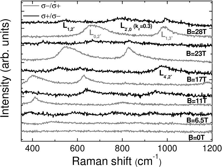
Figure 6: a) Representative Raman scattering spectra at different values of the magnetic field in $\sigma^{-}/\sigma^{+}$ (black curves) and $\sigma^{+}/\sigma^{-}$ (gray curves) configurations showing different magnetic field dependent features.

Most of the observed excitation fulfill the Raman scattering selection rules presented in the previous sections, but we also observe traces of optical-like excitations with $\Delta|n|=\pm 1$: $L_{1,2^{+}}$ in the $\sigma^{-}/\sigma^{+}$ configuration and $L_{3^{-},2^{+}}$ in the $\sigma^{+}/\sigma^{-}$.

All electronic excitations observed in the crossed polarization configuration are significantly weaker than the symmetric lines observed in co-circular configuration, but unexpectedly, in the $\sigma^{-}/\sigma^{+}$ polarization configuration two particular features involving the $n=0,1$ Landau levels are of much stronger intensity. These two features are presented in Fig. 6 (gray curves). They have a significantly different line shape, $L_{1,3^{+}}$ being asymmetric as the $\Delta|n|=0$ excitation discussed in the previous section, while the $L_{0,2^{+}}$ feature is much broader. Probably, the difference between these two features and the rest of $(n-1)^{-}\to(n+1)^{+}$ transitions can be explained by the different $k_{z}$ dispersion of the $n=0,1$ Landau levels.

In the $\sigma^{+}/\sigma^{-}$ polarization configuration $\Delta|n|=-2$ and possibly $\Delta|n|=+1$ excitations are expected. The feature with the lowest energy in this configuration is attributed to $L_{1,2^{+}}$ excitation at $k_{z}=0$. The first feature of the $\Delta|n|=-2$ series is the $L_{2^{-},0}$ excitation which should be blocked at $k_{z}=0$ due to the full occupation of the $n=0$ level, but $k_{z}\neq 0$ excitations can be observed. We attribute the broad feature with a much reduced amplitude as compared to the others (see Fig 6) to the $L_{2^{-},0}$ excitation at $k_{z}=k_{F}\sim 0.3$ (dotted lines in Fig. 5). The second excitation with the same change of Landau band modulus that could be expected is $L_{3^{-},1}$, which should also be blocked because of occupation effects in the $n=1$ level. This feature is not clearly observed in the present experiment.

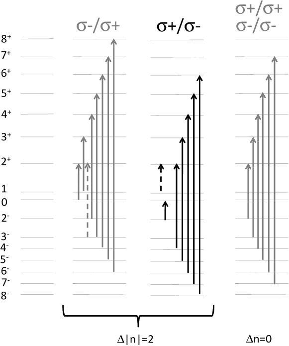
Figure 7: Schematics of the observed electronic excitations in the two crossed circular configurations and in co-circular configuration in natural graphite. Observed optical-like excitations are indicated by dashed arrows.

To summarize all the obtained results, we present in Fig. 7 a schematic picture of all the observed excitations in the different crossed- and co-circular polarization configurations. In the $\sigma^{-}/\sigma^{+}$ configuration electronic excitations with $\Delta|n|=+2$ are observed and traces of the optical-excitation $L_{3^{-},2^{+}}$. The two excitations involving the $0,1$ Landau levels also fulfill this index rule. In the $\sigma^{+}/\sigma^{-}$, $\Delta|n|=-2$ excitations are observed together with the optical-like excitation $L_{1,2^{+}}$ and of the symmetric excitation $L_{2^{-},2^{+}}$. The $\Delta|n|=\pm 1$ optical-like electronic excitations series are not clearly observed in this configuration but the coupling of these excitations with the $E_{2g}$ phonon has a strong influence on the phonon feature.

IV.3 Magneto-phonon effect in bulk graphite

To our knowledge, the magneto-phonon effect involving $K$-point massive carriers in bulk graphite and the $E_{2g}$ phonon has never been explored theoretically. This situation is of particular interest because of the nature of the electronic states involved in the coupling. The magneto-phonon effect in graphene Ando (2007a); Goerbig et al. (2007); Faugeras et al. (2009) or in bilayer graphene Ando (2007b) involves discrete electronic states which results in a fully resonant coupling with the phonon. In the case of $K$-point carriers in graphite, because of the 3D nature of bulk graphite and of the associated dispersion along $k_{z}$, the electronic states belong to Landau bands and the electronic excitation is spread over a wide range of energy (line width $\sim 50\,\mbox{cm}^{-1}$ in the case of symmetric lines in co-circular configuration) and the interaction is also spread on such a wide range of energy. As a result, we expect an effect less pronounced than in graphene and with asymmetric evolution of the parameters describing the phonon feature.

As already noticed in the previous section, the $E_{2g}$ phonon feature shows pronounced oscillations and even an anti-crossing behavior when optical electronic excitations $\Delta|n|=\pm 1$ (hardly seen in the Raman scattering experiment) are tuned in resonance with the phonon energy. This can be seen clearly in the lower panel of Fig. 4. We present in Fig. 8 raw Raman scattering spectra in the optical phonon range of energy for selected values of the magnetic field. The phonon feature energy and FWHM evolves a lot with magnetic field and at $B=28$ T a blue shift is clearly visible together with a strong broadening of the feature. It is possible to use Lorentzian curves to described these spectra, as shown by the dashed gray curves in Fig. 8. The parameters (namely, the peak position and its full width at half maximum) deduced from a Lorentzian fitting of the phonon feature as a function of the magnetic field are presented in Fig. 9(a) and (b) for the two crossed polarized configurations. The oscillations can be observed for magnetic fields higher than $B\sim 5$ T. One can note on Fig. 9(a) and (b) that the minima in FWHM or in Raman shift of the phonon feature in the two opposite crossed circular polarizations do not occur at the same values of the magnetic field. This difference is due to the electron-hole asymmetry in graphite discussed and determined in the previous section.

To describe the magneto-phonon effect theoretically, we adopt the same approach that was successfully used for the magneto-phonon effect in the monolayer graphene Faugeras et al. (2009); Yan et al. (2010). Namely, the shift and the broadening of the phonon are given by the real part and twice the imaginary part of the complex root $\omega$ of the equation

$$\omega^{2}-\omega_{0}^{2}=2\omega_{0}\lambda\left[\Pi_{B}(\omega+i\Gamma)-\Pi_{B=0}(\omega_{0}+i\Gamma)\right],$$ (6)

where $\Pi_{B}(\omega)$ is the polarization operator, which depends on the magnetic field and frequency. We have subtracted its value at $B=0$, so the shift is measured with respect to $\omega_{0}$, the phonon frequency at zero field (about $1583\>\mbox{cm}^{-1}$).

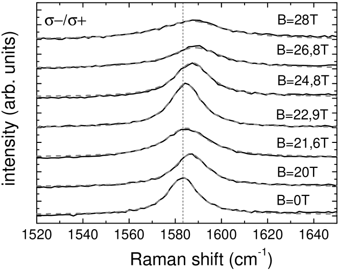
Figure 8: Raman scattering spectra at selected values of the magnetic field in the $\sigma^{-}/\sigma^{+}$ polarization configuration (solid black curves) and lorentizan curves (dashed gray curves). Curves are shifted for clarity. The vertical dashed line indicates the B=0 position.

The simplest two-parameter parabolic model, used in Sec. IV.1 to describe Raman scattering due to $\Delta|n|=0$ electronic excitations, is not sufficient to describe the magneto-phonon effect. Four-band approximation is needed, and transitions between levels involving the two split-off bands also need to be taken into account. The only approximation which is made here is to neglect the trigonal warping by setting $\gamma_{3}=0$. For each value of $B$, $k_{z}$, and of the Landau level index $n$, it is then sufficient to diagonalize a $4\times{4}$ matrix, instead of an infinite-dimensional one, which would be necessary for $\gamma_{3}\neq 0$. This significantly improves the computation efficiency, but introduces a certain error, that will be discussed in the following. Relegating the explicit expressions to Appendix A, we plot $\mathop{\mathrm{Re}}\nolimits\omega$ and $2\mathop{\mathrm{Im}}\nolimits\omega$ for the solutions of Eq. (6) by solid lines in Fig. 9. We have adjusted $\lambda=3.2\times{10}^{-3}$ and $\Gamma=44\>\mbox{cm}^{-1}$ to reproduce the amplitude of the oscillations and the degree of asymmetry. We added a constant broadening of $5\>\mbox{cm}^{-1}$ to $2\mathop{\mathrm{Im}}\nolimits\omega$ which corresponds to a broadening of the phonon by scattering mechanisms other than the electron-phonon interaction. We have used the SWM parameters listed in the left column of Table I, and set $\gamma_{3}=0$.

Setting $\gamma_{3}=0$ changes the inter-Landau-level excitation frequencies, so their resonance with the phonon occurs at slightly different values of the magnetic field and this explains why the minima and maxima of the theoretical and experimental curves are horizontally shifted in Fig. 9. In principle, one could remove this discrepancy by slightly readjusting other SWM parameters. However, this would introduce a correction to the transition matrix elements, and it is not clear whether they would be closer to their true values. Thus, we prefer to stick to the parameters from Table I, and consider the discrepancy between the resonance positions as an order-of-magnitude estimate of the error in the theory.

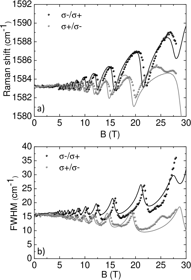
Figure 9: a) Raman shift and b) FWHM of the $E_{2g}$ phonon feature as a function of the magnetic field for the $\sigma^{-}/\sigma^{+}$ (black dots) and $\sigma^{+}/\sigma^{-}$ (gray dots) configurations.

The dependence of the magneto-phonon effect on the electronic Fermi energy, $\epsilon_{F}$, deserves a separate discussion. It enters $\Pi_{B}(\omega)$ through the filling of Landau levels $n=0,1$. Namely, all $n^{+}$ levels with $n\geq{2}$, as well as all levels from the upper split-off band are assumed to be empty, and all $n^{-}$ levels with $n\geq{2}$, as well as all levels from the lower split-off band are assumed to be filled. The $n=0$ and $n=1$ Landau levels are filled for $k_{z}<k_{0,1}^{F}$ and empty at $k_{z}>k_{0,1}^{F}$, where $k_{0}^{F}$, $k_{1}^{F}$ are those $k_{z}$ at which $n=0$ and $n=1$ Landau levels cross the Fermi level, $\epsilon_{0}=\epsilon_{F}$ and $\epsilon_{1}=\epsilon_{F}$, respectively. It turns out that these population effects are responsible for the smooth in $B$ component of the curves in Fig. 9, which is different for the two polarizations (the $\sigma^{-}/\sigma^{+}$ curve exhibits an overall increase in energy with $B$, while the $\sigma^{+}/\sigma^{-}$ an overall decrease). Indeed, (i) since there are no two $1^{+}$ and $1^{-}$ Landau levels, but a single one, only one of the two transitions $2^{-}\to{1}$, $1\to{2}^{+}$ is allowed for a given $k_{z}$, and the other one is blocked by the Pauli principle (assuming zero temperature); (ii) as the transitions $2^{-}\to{1}$, $1\to{2}^{+}$ contribute mainly in the $\sigma^{-}/\sigma^{+}$ and $\sigma^{-}/\sigma^{+}$ polarization, respectively, then, depending on the filling of the $n=1$ Landau level, the contribution is made in only one of the two polarizations. It turns out that the monotonous in $B$ component is mainly due to transitions around $k_{z}=\pi/2$ ($H$ point), which becomes resonant with the phonon at fields near $30\,\mbox{T}$. Indeed, the theoretical curves in Fig. 9 are very little sensitive to the value of $\epsilon_{F}$ as it is varied from $2\gamma_{2}$, the bottom of the conduction band at $k_{z}=0$ (when the $n=0,1$ levels are empty for all $k_{z}$), to $\gamma_{2}+30\,\mbox{meV}$, but when we fully populate the $n=0,1$ levels at all $k_{z}$ by pushing $k_{0,1}^{F}\to\pi/2$, the tendency is reversed: the $\sigma^{-}/\sigma^{+}$ curve decreases in energy with $B$, while the $\sigma^{+}/\sigma^{-}$ curve increases.

IV.4 Room Temperature Experiments

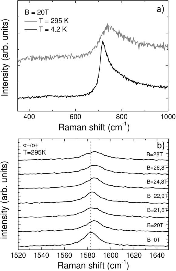
Figure 10: a) Raman scattering spectra measured at $T=4.2$ K (black curve) and at $T=295$ K (gray curve) at $B=20$ T in the $\sigma^{+}/\sigma^{+}$ configuration. b) Raman scattering spectra at selected values of the magnetic field in the $\sigma^{-}/\sigma^{+}$ polarization configuration measured at T=295K. Curves are shifted for clarity. The vertical dashed line indicates the B=0 position.

The results presented above have been extracted from low temperature ($4.2$ K) measurements. It is however instructive to note that that the magneto-Raman scattering response of graphite, which in fact reflects the quantum character of its energy structure, survives even at room temperature. We illustrate this here, although leave a more detailed discussion of temperature effects to a separate report.

Fig. 10a) shows the comparison of Raman scattering response due to $L_{2^{-},2^{+}}$ transition, measured at $4.2$ K and $295$ K, in co-circular configuration. At room temperature, the $L_{2^{-},2^{+}}$ spectrum is weaker but still clearly visible. The shift of the peak towards higher energies and its smearing observed at room temperature is due to thermal population of the final state $n=2^{+}$ Landau band. The low energy onset of the $L_{2^{-},2^{+}}$ spectrum remains rather sharp at low temperatures since all the $n=2^{+}$ Landau band is empty, down to $k_{z}=0$ states. Thermal population of $n=2^{+}$ band leads to Pauli blocking of the transitions, starting from those involving the $k_{z}=0$ final states, what quantitatively accounts for the shift and additional broadening of the $L_{2^{-},2^{+}}$ spectrum at elevated temperatures.

Remarkably, also the magneto-phonon resonance effect in graphite survives up to the room temperature. Room-temperature Raman scattering spectra measured in cross-polarization configuration and focused on the $E_{2g}$ phonon response are shown in Fig. 10b). The magneto-oscillations of the $E_{2g}$ phonon are clear at room temperature and resemble very much those measured at $4.2$ K, presented in Fig. 8.

Rough comparison of low and room-temperature data points towards thermal population effects being the main source of the observed difference in the spectral response. This implies that other possible sources of spectral broadening in magneto-Raman scattering of graphite have a negligible temperature dependence, extraordinarily, up to the room temperature.

V Conclusion

To conclude, we have used circularly polarized magneto-Raman scattering techniques in order to study purely electronic and phonon excitations in bulk graphite. Different series of electronic excitations arising from $K$-point carriers are observed. They are interpreted using the Raman scattering selection rules otherwise characteristic of the bilayer graphene. The use of polarized Raman scattering reveals a surprisingly strong electron-hole asymmetry and suggests that the generally accepted set of SWM parameters from Brandt et al. Brandt et al. (1988) under estimates the electron-hole asymmetry. The magneto-phonon effect is observed in the crossed circularly polarized configuration with different amplitude of the effect in the two distinct crossed polarized configurations due to the contribution of the holes at the H point of the graphite Brillouin zone. Electronic contributions to the Raman scattering spectrum of bulk graphite and the magneto-phonon effect are observed up to room temperature.

VI Acknowledgements

We acknowledge technical support from Ivan Breslavetz. Part of this work has been supported by ANR-08-JCJC-0034-01, GACR P204/10/1020, GRA/10/E006 (EPIGRAT), RTRA ”DISPOGRAPH” projects and by EuroMagNET II under the EU contract number 228043. P.K. is financially supported by the EU under FP7, contract no. 221515 ”MOCNA”. Yu. L. is supported by the Russian state contract No. 16.740.11.0146.

Appendix A Landau levels in the four-band model

The Hamiltonian of the $AB$-stacked graphite can be written as

$$H=\left(\begin{array}[]{cccccccccc}\ldots&\ldots&\ldots&\ldots&\ldots&\ldots&\ldots&\ldots&\ldots&\ldots\\ \ldots&V_{11}&V_{12}^{\dagger}&H_{1}&V_{12}^{\dagger}&V_{11}^{\dagger}&0&0&0&\ldots\\ \ldots&0&V_{22}&V_{12}&H_{2}&V_{12}&V_{22}^{\dagger}&0&0&\ldots\\ \ldots&0&0&V_{11}&V_{12}^{\dagger}&H_{1}&V_{12}^{\dagger}&V_{11}^{\dagger}&0&\ldots\\ \ldots&0&0&0&V_{22}&V_{12}&H_{2}&V_{12}&V_{22}^{\dagger}&\ldots\\ \ldots&\ldots&\ldots&\ldots&\ldots&\ldots&\ldots&\ldots&\ldots&\ldots\end{array}\right),$$ (7)

where each element is a matrix in the Hilbert space of a single layer. $H_{1}$ and $H_{2}$ contain the in-plane nearest-neighbor coupling with the matrix element $\gamma_{0}$ as well as the diagonal shift $\Delta$. $V_{12}$ represents the coupling between neighboring layers with matrix elements $\gamma_{1}$ for the neighboring atoms, and $\gamma_{3},\gamma_{4}$ for the second nearest neighbors. $V_{11}$ and $V_{22}$ correspond to second-nearest-layer coupling with matrix elements $\gamma_{2}/2$ and $\gamma_{5}/2$. Due to the translational invariance in the $z$ direction, the problem can be reduced to that of an effective bilayer:

$$H_{k_{z}}=\left[\begin{array}[]{cc}H_{1}+V_{11}e^{2ik_{z}}+V_{11}^{\dagger}{e}^{-2ik_{z}}&2V_{12}^{\dagger}\cos{k}_{z}\\ 2V_{12}\cos{k}_{z}&H_{2}+V_{22}e^{2ik_{z}a_{z}}+V_{22}^{\dagger}{e}^{-2ik_{z}a_{z}}\end{array}\right].$$ (8)

Here $k_{z}$ is the wave vector in the direction perpendicular to the layers, measured in the units of $1/a_{z}$, where $a_{z}$ is the distance between the neighboring layers. The period of the structure is $2a_{z}$, that is, two layers, so $-\pi/2<{k}_{z}\leq\pi/2$. Expansion of the single-layer Hamiltonian in $p_{x},p_{y}$, the in-plane quasi-momentum components counted from the $H-K-H$ line, gives

$${H}_{k_{z}}(\hat{\mathbf{p}})=\left[\begin{array}[]{cccc}\Gamma_{2}&v\hat{p}_{-}&-\alpha_{4}v\hat{p}_{-}&\alpha_{3}v\hat{p}_{+}\\ v\hat{p}_{+}&\Gamma_{5}&\Gamma_{1}&-\alpha_{4}v\hat{p}_{-}\\ -\alpha_{4}v\hat{p}_{+}&\Gamma_{1}&\Gamma_{5}&v\hat{p}_{-}\\ \alpha_{3}v\hat{p}_{-}&-\alpha_{4}v\hat{p}_{+}&v\hat{p}_{+}&\Gamma_{2}\end{array}\right],$$ (9)

where

$$v=\frac{3}{2}\,\frac{\gamma_{0}{a}}{\hbar},\quad\Gamma_{1}=2\gamma_{1}\mathcal{C},\quad\Gamma_{2}=2\gamma_{2}\mathcal{C}^{2},\quad\alpha_{3,4}=\frac{2\gamma_{3,4}}{\gamma_{0}}\,\mathcal{C},\quad\Gamma_{5}=2\gamma_{5}\mathcal{C}^{2}+\Delta,\quad\mathcal{C}\equiv\cos{k}_{z},$$ (10)

$a=1.42\>\mbox{\AA}$ is the distance between the neighboring carbon atoms in the same layer, and $\hat{p}_{\pm}=-i\hbar(\partial_{x}\pm{i}\partial_{y})$.

It is convenient to rotate the basis in the space of the 4-columns $(\psi_{1},\psi_{2},\psi_{3},\psi_{4})^{T}$ as

$$\psi_{1}^{\prime}=\frac{\psi_{2}+\psi_{3}}{\sqrt{2}},\quad\psi_{2}^{\prime}=\psi_{1},\quad\psi_{3}^{\prime}=\psi_{4},\quad\psi_{4}^{\prime}=\frac{\psi_{2}-\psi_{3}}{\sqrt{2}},$$ (11)

so the transformed Hamiltonian becomes

$$H^{\prime}_{k_{z}}(\hat{\mathbf{p}})=\left[\begin{array}[]{cccc}\Gamma_{5}+\Gamma_{1}&\bar{v}_{4}\hat{p}_{+}&\bar{v}_{4}\hat{p}_{-}&0\\ \bar{v}_{4}\hat{p}_{-}&\Gamma_{2}&\alpha_{3}v\hat{p}_{+}&v_{4}\hat{p}_{-}\\ \bar{v}_{4}\hat{p}_{+}&\alpha_{3}v\hat{p}_{-}&\Gamma_{2}&-v_{4}\hat{p}_{+}\\ 0&v_{4}\hat{p}_{+}&-v_{4}\hat{p}_{-}&\Gamma_{5}-\Gamma_{1}\end{array}\right],$$ (12)

where $v_{4}=v(1+\alpha_{4})/\sqrt{2}$, $\bar{v}_{4}=v(1-\alpha_{4})/\sqrt{2}$.

In the presence of a magnetic field, described by the vector potential in the Landau gauge $A_{x}=-By$, $A_{y}=A_{z}=0$, the wave functions can be sought in the form

$$\psi_{j}^{\prime}(x,y)=e^{ip_{x}x}\sum_{n=0}^{\infty}C_{j}^{(n)}\Phi_{n}(y+p_{x}l_{B}^{2}),$$ (13)

where $\Phi_{n}(y)$ are the harmonic oscillator wave functions. When $\gamma_{3}$ is finite, the coefficient $C_{j}^{(n)}$ is coupled to $C_{j}^{(n+3)}$, which, in turn, is coupled to $C_{j}^{(n+6)}$, and so on. In this situation, one can proceed either by perturbation theory or numerically. If we neglect $\gamma_{3}$ (set it to zero), the infinite-dimensional Hamiltonian splits into $4\times{4}$ blocks, corresponding to subspaces defined by

$$\left[\begin{array}[]{c}\psi_{1}^{\prime}\\ \psi_{2}^{\prime}\\ \psi_{3}^{\prime}\\ \psi_{4}^{\prime}\end{array}\right]=\left[\begin{array}[]{c}x_{1}^{(n)}\Phi_{n-1}\\ x_{2}^{(n)}\Phi_{n}\\ x_{3}^{(n)}\Phi_{n-1}\\ x_{4}^{(n)}\Phi_{n-1}\end{array}\right].$$ (14)

This greatly simplifies the calculation, as in each subspace we have a only a $4\times{4}$ eigenvalue problem (we denote $\epsilon_{B}=v/l_{B}$):

$$\left[\begin{array}[]{cccc}\Gamma_{5}+\Gamma_{1}-\epsilon&\sqrt{n}(1-\alpha_{4})\epsilon_{B}&\sqrt{n-1}(1-\alpha_{4})\epsilon_{B}&0\\ \sqrt{n}(1-\alpha_{4})\epsilon_{B}&\Gamma_{2}-\epsilon&0&\sqrt{n}(1+\alpha_{4})\epsilon_{B}\\ \sqrt{n-1}(1-\alpha_{4})\epsilon_{B}&0&\Gamma_{2}-\epsilon&-\sqrt{n-1}(1+\alpha_{4})\epsilon_{B}\\ 0&\sqrt{n}(1+\alpha_{4})\epsilon_{B}&-\sqrt{n-1}(1+\alpha_{4})\epsilon_{B}&\Gamma_{5}-\Gamma_{1}-\epsilon\end{array}\right]\left[\begin{array}[]{c}x_{1}^{(n)}\\ x_{2}^{(n)}\\ x_{3}^{(n)}\\ x_{4}^{(n)}\end{array}\right]=0.$$ (15)

For $\epsilon_{B}\ll\Gamma_{1}$, out of four eigenvalues, the largest one is of the order of $\Gamma_{1}$, and the lowest one is of the order of $-\Gamma_{1}$. These two correspond to split-off bands and are denoted by $\epsilon_{n^{++}}$, $\epsilon_{n^{--}}$, respectively. The other two, $\epsilon_{n^{+}}$ and $\epsilon_{n^{-}}$, correspond to those found in the two-band low-energy approximationMcCann and Fal’ko (2006). Eq. (15) is valid at $n\geq{2}$ only. At $n=1$ there are three states corresponding to $n=1$ with $x_{3}=0$ and energies $\epsilon_{1^{++}}\sim\Gamma_{1}$ $\epsilon_{1^{--}}\sim-\Gamma_{1}$, and $\epsilon_{1}$ with low energy. There is one state corresponding to $n=0$, with $x_{1}=x_{3}=x_{4}=0$ and $\epsilon_{0}=\Gamma_{2}$.

Optical transitions for each circular polarization are described by the operators $\hat{v}_{\pm}=(\hat{v}_{x}\pm{i}\hat{v}_{y})/\sqrt{2}$, where $\hat{v}_{x},\hat{v}_{y}$ are the components of the electronic velocity operator, $\hat{\mathbf{v}}=\partial{H}_{k_{z}}^{\prime}(\hat{\mathbf{p}})/\partial\hat{\mathbf{p}}$. The operator $\hat{v}_{+}$ has matrix elements only between the $n$ and $n-1$ manifolds:

$$\langle{n}-1|\frac{\hat{v}_{+}}{v}|n\rangle=(1-\alpha_{4})\left(x_{1}^{(n-1)}x_{3}^{(n)}+x_{2}^{(n-1)}x_{1}^{(n)}\right)+(1+\alpha_{4})\left(x_{2}^{(n-1)}x_{4}^{(n)}-x_{4}^{(n-1)}x_{3}^{(n)}\right),\quad n\geq{2},$$ (16)

$$\langle{0}|(\hat{v}_{+}/v)|1\rangle=(1-\alpha_{4})x_{1}^{(1)}+(1+\alpha_{4})x_{4}^{(1)}.$$ (17)

To obtain the polarization operator $\Pi_{B}(\omega)$, one has to sum up contributions from all $k_{z}$:

$$\Pi_{B}(\omega)=-\frac{1}{l_{B}^{2}}\int\limits_{-\pi/2}^{\pi/2}\frac{dk_{z}}{\pi}\,\sum_{n=0}^{\infty}\mathcal{P}_{n}(\omega,k_{z}),$$ (18)

where each $\mathcal{P}_{n}$ contains transitions between Landau levels from the $n$th and $(n+1)$st manifolds:

$$\mathcal{P}_{n\geq{2}}=\frac{|\langle{n}^{+}|\hat{v}_{+}|(n+1)^{-}\rangle|^{2}}{\epsilon_{n^{+}}-\epsilon_{(n+1)^{-}}\mp\omega}+\frac{|\langle{n}^{++}|\hat{v}_{+}|(n+1)^{-}\rangle|^{2}}{\epsilon_{n^{++}}-\epsilon_{(n+1)^{-}}\mp\omega}+\frac{|\langle{n}^{+}|\hat{v}_{+}|(n+1)^{--}\rangle|^{2}}{\epsilon_{n^{+}}-\epsilon_{(n+1)^{--}}\mp\omega}+\frac{|\langle{n}^{++}|\hat{v}_{+}|(n+1)^{--}\rangle|^{2}}{\epsilon_{n^{++}}-\epsilon_{(n+1)^{--}}\mp\omega}+$$

$$\hskip 28.45274pt{}+\frac{|\langle{n}^{-}|\hat{v}_{+}|(n+1)^{+}\rangle|^{2}}{\epsilon_{(n+1)^{+}}-\epsilon_{n^{-}}\pm\omega}+\frac{|\langle{n}^{-}|\hat{v}_{+}|(n+1)^{++}\rangle|^{2}}{\epsilon_{(n+1)^{++}}-\epsilon_{n^{-}}\pm\omega}+\frac{|\langle{n}^{--}|\hat{v}_{+}|(n+1)^{+}\rangle|^{2}}{\epsilon_{(n+1)^{+}}-\epsilon_{n^{--}}\pm\omega}+\frac{|\langle{n}^{--}|\hat{v}_{+}|(n+1)^{++}\rangle|^{2}}{\epsilon_{(n+1)^{++}}-\epsilon_{n^{--}}\pm\omega},\qquad$$ (19)

$$\mathcal{P}_{1}=\theta(k_{z}-k_{1}^{F})\left(\frac{|\langle{1}|\hat{v}_{+}|2^{-}\rangle|^{2}}{\epsilon_{1}-\epsilon_{2^{-}}\mp\omega}+\frac{|\langle{1}|\hat{v}_{+}|2^{--}\rangle|^{2}}{\epsilon_{1}-\epsilon_{2^{--}}\mp\omega}\right)+\frac{|\langle{1}^{++}|\hat{v}_{+}|2^{--}\rangle|^{2}}{\epsilon_{1^{++}}-\epsilon_{2^{--}}\mp\omega}+$$

$$\hskip 28.45274pt{}+\theta(k_{1}^{F}-k_{z})\left(\frac{|\langle{1}|\hat{v}_{+}|2^{+}\rangle|^{2}}{\epsilon_{2^{+}}-\epsilon_{1}\pm\omega}+\frac{|\langle{1}|\hat{v}_{+}|2^{++}\rangle|^{2}}{\epsilon_{2^{++}}-\epsilon_{1}\pm\omega}\right)+\frac{|\langle{1}^{--}|\hat{v}_{+}|2^{++}\rangle|^{2}}{\epsilon_{2^{++}}-\epsilon_{1^{--}}\pm\omega},$$ (20)

$$\mathcal{P}_{0}=\theta(k_{z}-k_{0}^{F})\,\frac{|\langle{0}|\hat{v}_{+}|1^{--}\rangle|^{2}}{\epsilon_{0}-\epsilon_{1^{--}}\mp\omega}+\theta(k_{0}^{F}-k_{z})\,\frac{|\langle{0}|\hat{v}_{+}|1^{++}\rangle|^{2}}{\epsilon_{1^{++}}-\epsilon_{0}\pm\omega}+\theta(k_{z}-k_{1}^{F})\,\theta(k_{0}^{F}-k_{z})\,\frac{|\langle{0}|\hat{v}_{+}|1\rangle|^{2}}{\epsilon_{1}-\epsilon_{0}\pm\omega}.$$ (21)

The upper and lower $\pm$ signs in the denominators correspond to $\sigma^{-}/\sigma^{+}$ and $\sigma^{+}/\sigma^{-}$ polarizations, respectively. Both the electronic energies and the velocity matrix elements depend on $B$ and $k_{z}$. The Fermi wave vectors $k_{0}^{F}(B)$, $k_{1}^{F}(B)$ are those $k_{z}$ at which $n=0$ and $n=1$ Landau levels match the Fermi energy, $\epsilon_{0}=\epsilon_{F}$ and $\epsilon_{1}=\epsilon_{F}$, respectively. The sum over $n$ in Eq. (18) is divergent, so we cut it off at a certain energy $\epsilon_{\mathrm{max}}$. Namely, for transitions not involving the split-off bands, we sum over those $n$ for which $\epsilon_{(n+1)^{+}}<\epsilon_{\mathrm{max}}$. Transitions involving the split-off bands are counted if $\epsilon_{(n+1)^{++}}<\epsilon_{\mathrm{max}}$. The subsequent integration over $k_{z}$ is performed numerically. The results presented in Sec. V were obtained with $\epsilon_{\mathrm{max}}=1\,\mbox{eV}$, and we have verified that the difference $\Pi_{B}(\omega)-\Pi_{B=0}(\omega_{0})$ does not depend on $\epsilon_{\mathrm{max}}$.

References

- Galt et al. (1956) J. Galt, W. Yager, and H. Dail, Phys. Rev. 103, 1586 (1956).
- Schroeder et al. (1968) P. R. Schroeder, M. S. Dresselhaus, and A. Javan, Phys. Rev. Lett. 20, 1292 (1968).
- Toy et al. (1977) W. W. Toy, M. S. Dresselhaus, and G. Dresselhaus, Phys. Rev. B 15, 4077 (1977).
- Li et al. (2006) Z. Q. Li, S.-W. Tsai, W. J. Padilla, S. V. Dordevic, K. S. Burch, Y. J. Wang, and D. N. Basov, Phys. Rev. B 74, 195404 (2006).
- Sadowski et al. (2006) M. L. Sadowski, G. Martinez, M. Potemski, C. Berger, and W. A. de Heer, Phys. Rev. Lett. 97, 266405 (2006).
- Jiang et al. (2007) Z. Jiang, E. A. Henriksen, L. C. Tung, Y. J. Wang, M. E. Schwartz, M. Y. Han, P. Kim, and H. L. Stormer, Phys. Rev. Lett. 98, 197403 (2007).
- Orlita et al. (2008a) M. Orlita, C. Faugeras, P. Plochocka, P. Neugebauer, G. Martinez, D. K. Maude, A. L. Barra, M. Sprinkle, C. Berger, W. A. de Heer, and M. Potemski, Phys. Rev. Lett. 101, 267601 (2008a).
- Orlita et al. (2008b) M. Orlita, C. Faugeras, G. Martinez, D. K. Maude, M. L. Sadowski, and M. Potemski, Phys. Rev. Lett. 100, 136403 (2008b).
- Henriksen et al. (2007) E. A. Henriksen, Z. Jiang, L. C. Tung, M. E. S. M. Takita, Y. J. Wang, P. Kim, and H. L. Stormer, Phys. Rev. Lett. 100, 087403 (2007).
- Orlita et al. (2009) M. Orlita, C. Faugeras, J. Schneider, G. Martinez, D. K. Maude, and M. Potemski, Phys. Rev. Lett. 102, 166401 (2009).
- Chuang et al. (2009) K. C. Chuang, A. M. R. Baker, and R. J. Nicholas, Phys. Rev. B 80, 161410(R) (2009).
- Orlita and Potemski (2010) M. Orlita and M. Potemski, Semicond. Sci. Technol. 25, 063001 (2010).
- Faugeras et al. (2011) C. Faugeras, M. Amado, P. Kossacki, M. Orlita, M. Kuhne, A. Nicolet, Y. Latyshev, and M. Potemski, Phys. Rev. Lett. 107, 036807 (2011).
- Dresselhaus et al. (2010) M. Dresselhaus, A. Jorio, and R. Saito, Annu. Rev. Condens. Matter Phys. 1, 89 (2010).
- Ando (2007a) T. Ando, J. Phys. Soc. Jpn. 76, 024712 (2007a).
- Goerbig et al. (2007) M. O. Goerbig, J. N. Fuchs, K. Kechedzhi, and V. Fal’ko, Phys. Rev. Lett. 99, 087402 (2007).
- Kashuba and Fal’ko (2009) O. Kashuba and V. I. Fal’ko, Phys. Rev. B 80, 241404(R) (2009).
- Mucha-Kruczynski et al. (2010) M. Mucha-Kruczynski, O. Kashuba, and V. I. Fal’ko, Phys. Rev. B 82, 045405 (2010).
- Faugeras et al. (2009) C. Faugeras, P. Kossacki, M. Amado, M. Orlita, M. Sprinkle, C. Berger, W. A. de Heer, and M. Potemski, Phys. Rev. Lett. 103, 186803 (2009).
- Yan et al. (2010) J. Yan, S. Goler, T. D. Rhone, M. Han, R. He, P. Kim, V. Pellegrini, and A. Pinczuk, Phys. Rev. Lett. 105, 227401 (2010).
- Garcia-Flores et al. (2009) A. F. Garcia-Flores, H. Terashita, E. Granado, and Y. Kopelevich, Phys. Rev. B 79, 113105 (2009).
- Slonczewski and Weiss (1958) J. C. Slonczewski and P. R. Weiss, Phys. Rev. 109, 272 (1958).
- McClure (1956) J. W. McClure, Phys. Rev. 104, 666 (1956).
- Li et al. (2009a) G. Li, A. Luican, and E. Y. Andrei, Phys. Rev. Lett. 102, 176804 (2009a).
- Neugebauer et al. (2009) P. Neugebauer, M. Orlita, C. Faugeras, A.-L. Barra, and M. Potemski, Phys. Rev. Lett. 103, 136403 (2009).
- Nakao (1976) K. Nakao, J. Phys. Soc.Jpn. 40, 761 (1976).
- Soule (1958) D. E. Soule, Phys. Rev. 112, 698 (1958).
- Soule et al. (1964) D. E. Soule, J. W. McClure, and L. B. Smith, Phys. Rev. 134, A453 (1964).
- Woollam (1970) J. A. Woollam, Phys. Rev. Lett. 25, 810 (1970).
- Schneider et al. (2009) J. M. Schneider, M. Orlita, M. Potemski, and D. K. Maude, Phys. Rev. Lett. 102, 166403 (2009).
- Abergel and Fal ko (2007) D. Abergel and V. Fal ko, Phys. Rev. B 75, 155430 (2007).
- Partoens and Peeters (2007) B. Partoens and F. M. Peeters, Phys. Rev. B 75, 193402 (2007).
- Koshino and Ando (2008) M. Koshino and T. Ando, Phys. Rev. B 77, 115313 (2008).
- Basko (2008) D. M. Basko, Phys. Rev. B 78, 125418 (2008).
- Basko (2009) D. M. Basko, New. J. Phys. 11, 095011 (2009).
- Ando (2007b) T. Ando, J. Phys. Soc. Jpn. 76, 104711 (2007b).
- Li et al. (2009b) Z. Li, E. Henriksen, Z. Jiang, Z. Hao, d. P. K. M.C. Martin a, H. Stormer, and D. Basov, Nature Phys. 4, 532 (2009b).
- Brandt et al. (1988) N. Brandt, S. Chudinov, and Y. Ponomarev, Semimetals 1: Graphite and its Compounds, edited by North-Holland (1988).
- McCann and Fal’ko (2006) E. McCann and V. Fal’ko, Phys. Rev. Lett. 96, 086805 (2006).