The GALEX Arecibo SDSS Survey. IV. Baryonic Mass-Velocity-Size Relations of Massive Galaxies
Abstract
We present dynamical scaling relations for a homogeneous and representative sample of 500 massive galaxies, selected only by stellar mass ( M⊙) and redshift () as part of the ongoing GALEX Arecibo SDSS Survey. We compare baryonic Tully-Fisher (BTF) and Faber-Jackson (BFJ) relations for this sample, and investigate how galaxies scatter around the best fits obtained for pruned subsets of disk-dominated and bulge-dominated systems. The BFJ relation is significantly less scattered than the BTF when the relations are applied to their maximum samples (for the BTF, only galaxies with Hi detections), and is not affected by the inclination problems that plague the BTF. Disk-dominated, gas-rich galaxies systematically deviate from the BFJ relation defined by the spheroids. We demonstrate that by applying a simple correction to the stellar velocity dispersions that depends only on the concentration index of the galaxy, we are able to bring disks and spheroids onto the same dynamical relation — in other words, we obtain a generalized BFJ relation that holds for all the galaxies in our sample, regardless of morphology, inclination or gas content, and has a scatter smaller than 0.1 dex. We compare the velocity-size relation for the three dynamical indicators used in this work, i.e., rotational velocity, observed and concentration-corrected stellar dispersion. We find that disks and spheroids are offset in the stellar dispersion-size relation, and that the offset is removed when corrected dispersions are used instead. The generalized BFJ relation represents a fundamental correlation between the global dark matter and baryonic content of galaxies, which is obeyed by all (massive) systems regardless of morphology.
keywords:
galaxies: kinematics and dynamics – galaxies: evolution – galaxies: fundamental parameters – radio lines: galaxies1 Introduction
The observed global properties of galaxies obey a diverse set of scaling relations, which are fundamental tools to constrain models of galaxy formation and evolution. Particularly interesting are the correlations between dynamics and luminosity/stellar mass or size, such as the Tully-Fisher (TF; Tully & Fisher, 1977) relation for spirals, and the Faber-Jackson (FJ; Faber & Jackson, 1976), - (Dressler et al., 1987), or fundamental plane (FP; Djorgovski & Davis, 1987; Dressler et al., 1987) relations for spheroids, because they link the luminous to the total mass of galaxies, thus providing insights into the interplay between their baryonic and dark matter components.
Historically, the importance of the tight TF and FP relations as secondary distance indicators has driven the community to assemble galaxy samples that meet strict selection criteria, in order to minimize systematic errors and scatter. While FP studies targeted elliptical and S0 galaxies, the samples used for TF applications have typically been restricted to late-type spirals with inclinations to the line-of-sight larger than 30-40∘, preferably observed in red or infrared photometric bands to minimize extinction effects (e.g., Courteau, 1997; Giovanelli et al., 1997b; Masters et al., 2006). These data sets are not ideal for characterizing the statistical properties of galaxies in general, because the excessive pruning means that they are not fair samples of the local Universe. This issue is particularly problematic for the comparison with theoretical studies and numerical simulations of galaxy formation and evolution, which should be based on representative samples. For instance, TF studies of different classes of objects, such as S0s and early-type spirals (e.g., Neistein et al., 1999; Bedregal et al., 2006; Williams et al., 2010, and references therein), polar ring galaxies (Iodice et al., 2003), barred spirals (Courteau et al., 2003), and gas-rich dwarfs (McGaugh et al., 2000; Begum et al., 2008), have sometimes found disagreement with the TF relation of late-type spirals. Most notably, gas-rich dwarfs lie systematically below the TF relation defined by bright galaxies.
During the last decades, the interest in TF and FJ-like scaling relations has shifted from cosmic flow applications to constraining galaxy formation models, and samples with broader morphological properties have been constructed specifically for this purpose (e.g., Kannappan et al., 2002; Pizagno et al., 2007; Dutton et al., 2007; Avila-Reese et al., 2008). However, current large and homogeneous data sets include either spirals (e.g., in addition to the works mentioned above, Courteau et al. 2007a and Saintonge & Spekkens 2011, hereafter SS11) or early-type galaxies (e.g., Bernardi et al., 2003; Graves et al., 2009) only.
There have been attempts to move beyond the spiral/elliptical dichotomy, and uncover relations between stellar content and dynamics that hold for all galaxies, independent of morphology. Zaritsky et al. (2008) found that all galaxies, from disks to spheroids and from dwarf spheroidals to giant ellipticals, lie on a two-dimensional surface defined by surface brightness, half-light radius, internal velocity and mass-to-light ratio. As a measure of internal velocity , they adopt either the rotational velocity for disks or the velocity dispersion for spheroids, thus the two types of systems are still treated separately (especially because the sample is a large but heterogeneous collection of published data sets, for which either or is available).
It is also important to point out that the search for scaling relations that are valid for all types of galaxies should make use of baryonic masses (i.e., the sum of stellar and gas masses) instead of luminosities or stellar masses, because they could be more fundamental quantities. This is demonstrated by the fact that baryonic scaling relations hold for subsets of galaxies that do not follow the corresponding stellar relations. For example, the offset of the gas-rich dwarf galaxies from the stellar TF relation disappears when their gas mass is taken into account (McGaugh et al., 2000; Begum et al., 2008). The baryonic TF relation (BTF; McGaugh et al., 2000) is linear over 5 orders of magnitude in (stellar + gas) mass, suggesting that the TF is fundamentally a relation between baryonic (rather than luminous) and total mass of the galaxy. Intriguingly, although supported by limited statistics, there is some evidence that giant and dwarf ellipticals might lie on the same BTF as the spirals (De Rijcke et al., 2007). Unfortunately, because they require estimates of both stellar and gas masses, BTF samples (e.g., McGaugh, 2005; Geha et al., 2006; Begum et al., 2008; Gurovich et al., 2004, 2010) are significantly smaller than TF ones.
To summarize, it is still unclear if disk-dominated galaxies and spheroids obey the same dynamical scaling relations, mainly due to the lack of well-defined, representative samples of galaxies for which both rotation and stellar dispersion are measured. Certainly, ellipticals might have no gas and no detectable rotation, and pure disks might have negligible stellar dispersions, but a significant fraction of local galaxies (especially massive ones) have a disk and a bulge (e.g. Driver et al., 2007), and the dynamical scaling relations should account for the smooth transition across galaxies with different bulge-to-disk ratios. As Covington et al. (2010) point out, a connection between the scaling relations of early-type and late-type galaxies is expected on the grounds that early-type systems are generally assumed to form through mergers of late-type ones. This is especially true at the high stellar mass end, where the blue sequence of star-forming disks merges onto the red sequence of passively-evolving, bulge-dominated galaxies (e.g. Baldry et al., 2006), and the systems typically host a bulge and a disk.
In this paper, we investigate dynamical scaling relations for a representative sample of 500 massive galaxies that are selected only by stellar mass ( M⊙) and redshift (), as part of the ongoing GALEX Arecibo SDSS Survey (GASS; Catinella et al., 2010, hereafter Paper I). For these galaxies, we have homogeneous measurements of structural parameters and velocity dispersions from the Sloan Digital Sky Survey (SDSS; York et al., 2000), NUV colours from GALEX (Martin et al., 2005) and SDSS imaging, and Hi masses and rotational velocities for the subset of objects detected at 21 cm with the Arecibo radio telescope. This unique sample, which includes massive galaxies of all morphological types, allows us to investigate how objects that are typically not included in TF or FJ/FP data sets scatter around those relations. In the spirit of works like those of Zaritsky et al. (2008) and Covington et al. (2010), we wish to establish if there is a fundamental correlation between baryonic mass and dynamics that is obeyed by the complete galaxy population, regardless of morphology. We show that, at least for the massive galaxies in our sample, such a relation does exist, and has a scatter smaller than 0.1 dex, comparable to that of the TF and FJ relations applied to their respective pruned subsets.
This paper is organized as follows. We summarize sample selection and measurements of relevant quantities in § 2. We present the baryonic mass-velocity relations, starting with the TF and FJ, in § 3, and the velocity-size relations in § 4. We discuss our findings and conclude in § 5.
All the distance-dependent quantities in this work are computed assuming , and km s-1 Mpc-1.
2 Sample Selection and Galaxy Parameters
The sample used in this work is drawn from GASS, an on-going survey which is gathering high-quality Hi-line spectra for 1000 massive galaxies, selected only by stellar mass (greater than M⊙) and redshift (). The GASS targets are located within the intersection of the footprints of the SDSS primary spectroscopic survey, the projected GALEX Medium Imaging Survey and the on-going Hi blind Arecibo Legacy Fast ALFA (ALFALFA; Giovanelli et al., 2005) survey. The galaxies are observed with the Arecibo radio telescope until detected or until a gas fraction limit of % is reached. For more details we refer the reader to Paper I, where the first GASS data release (DR1) is presented.
Here, in addition to the DR1 data (176 galaxies), we use new Arecibo observations of 240 galaxies that will be incorporated in the second GASS data release (Catinella et al., in preparation). As discussed in Paper I, GASS does not re-observe objects with good Hi detections already available from the ALFALFA survey or the Cornell Hi archive (Springob et al., 2005, hereafter S05). To correct the GASS sample for its lack of Hi-rich objects, we add galaxies from ALFALFA and S05 in the correct proportions, following the procedure detailed in section 7.2 of Paper I. The sample thus obtained, which is representative in terms of Hi properties, includes 480 galaxies (296 detections and 184 non-detections). As explained below, we discard 44 galaxies for which the stellar velocity dispersion is not reliable. The final sample includes 436 galaxies (259 detections and 177 non-detections).
As mentioned in Paper I, the optical parameters are obtained from queries to the SDSS DR7 (Abazajian et al., 2009) data base server, unless otherwise noted. Stellar masses are derived from SDSS photometry using the spectral energy distribution (SED) fitting technique described in Salim et al. (2007), assuming a Chabrier (2003) initial mass function. A variety of model SEDs from the Bruzual & Charlot (2003) library are fitted to each galaxy, building a probability distribution for its stellar mass. The mean and the width of this distribution are used as measurements of the stellar mass and its formal error, respectively. Over the interval probed by GASS, stellar masses are believed to be accurate to better than 30 per cent. As a measure of galaxy size we adopt , i.e. half the 25 mag arcsec-2 isophote diameter (measured by us on the SDSS g-band images), in kpc.
The baryonic mass is the sum of stars and gas; the latter is computed from the Hi mass, adopting the standard 1.4 correction factor to account for helium and metals, i.e. . This correction neglects the contribution of the molecular hydrogen. In our stellar mass regime, the amount of does not depend significantly on or concentration index and, on average, (but with a large scatter, 0.41 dex; Saintonge et al. 2011). Since the contribution of the Hi to the baryonic mass is, for our sample, typically small (see § 3.1), it is safe to neglect the (but we did check that including the molecular gas does not change our results). We set the Hi masses of the non-detections to zero, but we note that using the upper limits (which correspond to 1.5-5% of the stellar mass by survey design) would make no difference to our plots. Other parameters used in this work are discussed below.
2.1 Hi line widths
Hi line widths from GASS, ALFALFA and the S05 archive are measured with the same technique, at the 50% of each peak level (e.g., Catinella et al., 2007, §2.2). However, the corrections applied to the raw measurements, as originally published, are different. GASS and S05 widths are corrected for both instrumental broadening and cosmological redshift, whereas ALFALFA widths are corrected for instrumental broadening only, following equation 1 in Kent et al. (2008). No turbulent motion or inclination corrections are applied. For convenience, we report here the corrections adopted:
where is the measured velocity width, is the galaxy redshift, and is the instrumental broadening correction, which differs for the three sources. For GASS Paper I and ALFALFA, is simply the final velocity resolution of the spectrum after smoothing (i.e., between 5 and 21 km s-1 for GASS spectra, which are Hanning and boxcar smoothed, and 10 km s-1 for ALFALFA spectra, which are Hanning smoothed only). For S05, equals , where is the channel separation in km s-1 and is a complex function of signal-to-noise ratio (SNR) and type of smoothing applied. For high SNR, Hanning-smoothed spectra with km s-1 (i.e., the ALFALFA case), , thus is of order of half the velocity resolution after smoothing. This is smaller than the correction adopted for GASS in Paper I, and larger than the ALFALFA one, where the subtraction in quadrature makes the correction negligible (i.e., km s-1) for velocity widths larger than 50 km s-1.
The issue of homogenizing velocity widths obtained from different sources has been discussed in the past, and most recently by Courtois et al. (2009) for the Extragalactic Distance Database (Tully et al., 2009), a large compilation of data for galaxy distance and peculiar motion studies. We follow Courtois et al. (2009), who adopt a simplified version of the S05 solution, i.e.: , where and is the final velocity resolution of the spectrum after smoothing (this is half the correction adopted in Paper I). This is in better agreement with our own tests on high SNR GASS Hi profiles, where the smoothing was gradually increased and the width remeasured. Thus, we keep the S05 widths as published111 For the only galaxy in common between S05 and GASS (GASS 38751, AGC 240702), the corrected velocity widths agree within the quoted errors. , we adopt the new correction for the GASS data, and we uncorrect the ALFALFA widths, , to obtain the raw measurements, then apply the same and corrections adopted for GASS galaxies.
Lastly, we deproject all velocity widths to edge-on view. The inclination to the line-of-sight is computed from:
| (1) |
where is the minor-to-major axis ratio from the r-band exponential fit (expAB_r in the SDSS database), and is the intrinsic axial ratio of a galaxy seen edge-on. We adopt (Holmberg 1958; see also, e.g. Tully et al. 2009), and set the inclination to 90∘ for galaxies with . The value of applies to galaxies of morphological type earlier than Sbc, whereas should be used for Sbc and later spirals (e.g. Giovanelli et al. 1994, 1997a; SS11). However the difference is small, and our choice of seems appropriate for a sample of massive galaxies that was not selected for TF studies.
Thus, rotational velocities are computed as:
| (2) |
where is the final velocity resolution of the spectrum after smoothing.
As noted in Paper I, the Hi masses of galaxies in the ALFALFA and S05 archives have been recomputed from the tabulated fluxes, in order to be made consistent with GASS ones.
We identified 31 galaxies for which Hi confusion within the 4′ Arecibo beam is certain, and therefore the measured Hi parameters should not be trusted. Specifically, we closely inspected the SDSS images of all the galaxies in our sample, and flagged as “confused” those with at least one late-type, similar size companion (based on SDSS spectroscopy, i.e. with redshift available and within 0.002 of that of the target galaxy) within the beam. These objects will be highlighted in our analysis when needed.
2.2 Velocity dispersions
Galaxy velocity dispersions are measured by fitting stellar templates convolved with Gaussian functions to SDSS spectra, which are obtained through 3″-diameter fiber apertures. Because the fiber covers only a fraction of the galaxy light at the GASS redshifts, these quantities (catalogued as velDisp in the SDSS spectroscopic data base, and here referred to as ) need to be corrected for aperture effects. As commonly done (see, e.g. Bernardi et al., 2003; Graves et al., 2009, and references therein), fiber velocity dispersions are corrected to 1/8 effective radius as follows:
| (3) |
where and is the circular galaxy radius in arcseconds, computed as ( and are the effective radius and axis ratio from the r-band de Vaucouleurs fit, respectively). This correction is small, 3% on average, for the galaxies in our sample.
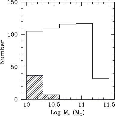
Only values of above the 70 km s-1 instrumental resolution of the SDSS spectra are considered reliable. We thus discarded 44 galaxies that do not meet this requirement from our sample; the effect of this restriction on the stellar mass distribution of the sample is shown in Figure 1.
3 Baryonic Mass-Velocity Relations
The main goal of this work is to establish if there is a relation between baryonic mass and a measure of the dynamical mass (estimated based on rotational velocity, stellar dispersion or a combination of the two) that is obeyed by massive galaxies regardless of their morphology.
We begin by comparing the baryonic TF (BTF) and baryonic FJ (BFJ) relations for our sample, in order to establish which quantity, the Hi rotational velocity or the stellar dispersion, most reliably traces the baryonic mass of massive galaxies. Thanks to its unique selection by stellar mass and redshift only, the GASS sample includes massive galaxies of all morphological types, and it is thus ideal for this comparison. Indeed, this is not a sample designed for either TF or FJ studies, but we can prune it to separately study inclined, disk-dominated and spheroidal, bulge-dominated systems. Most importantly, we can investigate outliers and residuals of the BTF and BFJ relations, which is essential in order to determine how to bring disks and spheroids onto the same relation. We conclude by illustrating two different ways of obtaining a baryonic relation that holds for all the massive galaxies in our sample, and whose dispersion is comparable to that of the BTF and BFJ relations.
3.1 Baryonic Tully-Fisher Relation
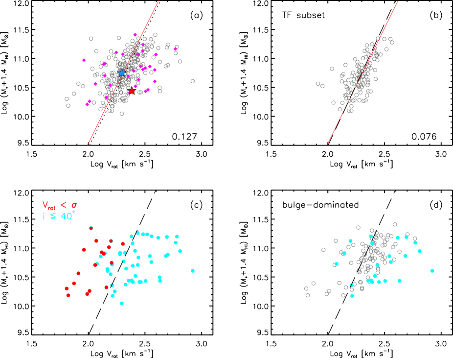
Here we must restrict our sample to galaxies with Hi detections, for which the rotational velocity can be measured. The BTF relation for this sample is shown in Figure 2a. We note that, for our interval of stellar masses, the contribution of the gas to the baryonic mass is generally small — if we plotted stellar instead of baryonic masses, most of the points would move downward by an amount comparable to the symbol size (indeed, there are only 13 galaxies in our sample with gas fractions /). We plot the BTF as usually done (i.e., baryonic mass versus rotational velocity), but we fit the inverse relation, since the scatter is clearly associated to the -coordinate (as can be seen by comparing Figures 2a and 2b, explained below). The inverse fit to the data points, i.e. Log = a Log (+ 1.4 ) + b, is shown as a dotted line222 Tables 1 and 2 list the expression of the fit, the scatter, and the number of galaxies contributing to the sample for all the main relations discussed in this work. . Following SS11, we compute the scatter in the variable around the best fit by applying Tukey’s bi-weight, which yields a robust estimate of the dispersion in presence of outliers; the scatter (in dex of velocity) is noted at the bottom of the panel. Also shown is the relation obtained by McGaugh et al. (2000) over nearly 5 orders of magnitude of baryonic mass (solid line), which is in excellent agreement with our data.
Not surprisingly, the scatter around the best fit is large for our data set (0.127 dex), and discarding galaxies with confused Hi spectra (magenta symbols; see § 2.1) improves it only by a small amount (0.112 dex). However, we recover a significantly tighter relation when we prune the sample as usually done for TF studies. This is illustrated in Figure 2b, where a TF subset was obtained by selecting non-confused, disk-dominated, inclined galaxies (i.e., objects with concentration index and inclination ∘; the scatter of the BTF for this subset is 0.076 dex). We inspected the three low-velocity outliers that stand out on the left of the plot. Two of them are galaxies for which the SDSS inclination is clearly overestimated (we measured 17∘ and 26∘ instead of 46∘ and 49∘, respectively), and the third one has uncertain Hi velocity width. Removing these outliers, the scatter of the relation becomes 0.072 dex. How does this compare with the scatter of other TF samples? There is a vast literature on the TF relation, showing that its scatter depends on the sample analyzed, velocity indicator, photometric band, and type of fit performed (forward, inverse, bisector or orthogonal). McGaugh (2005) studied the BTF relation using a sample of 60 galaxies with extended Hi rotation curves, and obtained a scatter of 0.191 dex in solar masses from a direct fit (this is the average scatter for the relations marked as in his Table 2, where the stellar masses are computed using stellar population synthesis models as we do). For comparison, a direct fit to the data in Figure 2b (excluding the three low-velocity outliers mentioned above) yields a scatter of 0.221 dex in solar masses. A study that is directly comparable to ours is that of Avila-Reese et al. (2008), who measured a scatter of 0.06 dex in velocity for the BTF of a sample of 76 non-interacting disk galaxies, with inclinations and flat rotation curves (see also, e.g., Pizagno et al., 2007). Given the crude selection of our TF subset (by concentration index), our sample is likely to include a broader range of disk galaxy types, thus the slightly larger scatter compared to these studies is not unexpected.
Figure 2c demonstrates that the high-velocity outliers of the BTF relation are all galaxies with small inclination to the line-of-sight. For these systems, the corrected rotational velocities become so unreliable that the correlation with baryonic mass effectively disappears. Once galaxies with inclination smaller than 40∘ are removed from the sample, even bulge-dominated objects lie reasonably close to the relation obtained for disk-dominated ones, although with larger scatter (empty circles in Fig. 2d). This agrees qualitatively with the findings of Ho (2007), based on a compilation of 792 galaxies with inclination larger than 30∘ and heterogeneous measurements from Hyperleda (Paturel et al., 2003a, b). Indeed, Ho showed that a -band TF relation exists for all Hubble types, including elliptical and S0 galaxies (although these represent a very small fraction of his sample).
Figure 2c also shows a population of low-velocity outliers that cannot be explained by small inclinations: these are galaxies with rotational velocities that are smaller than the stellar velocity dispersions (red symbols). We note that Ho (2007) also identifies a population of galaxies with unusually small ratios, which are outliers in his TF relation. Except for their small rotational velocities compared to their central stellar velocity dispersions, his outliers are otherwise normal luminous galaxies. These systems might be very interesting — Ho argues that a significant fraction of their Hi gas must be dynamically unrelaxed, having been acquired through a minor merger episode or perhaps cold accretion. For our sample, the fraction of low outliers is smaller (5%, against 17% for Ho’s sample). As shown in the Appendix, where these galaxies are described in more detail, most of them have asymmetric Hi profiles, suggesting that the Hi distribution and/or kinematics might be disturbed (although we cannot prove that the gas was externally accreted).
Lastly, here and in other figures of this paper we highlight the positions of two interesting galaxies that were discussed in our previous works, GASS 3505 and 35981 (marked as a red and a blue star in Fig. 2a). These are both unusually Hi-rich systems, which are outliers in the gas fraction plane discussed in Paper I (relating the Hi mass fraction to stellar mass surface density and NUV color). However, GASS 3505 is an early-type system, whereas GASS 35981 (UGC 8802) is a disk galaxy with a sharp metallicity drop in its outer disk, which suggests an external origin for the Hi gas (Moran et al. 2010; see also Wang et al. 2011). As can be seen, from a dynamical point of view GASS 35981 is not unusual, whereas GASS 3505 is still an outlier.
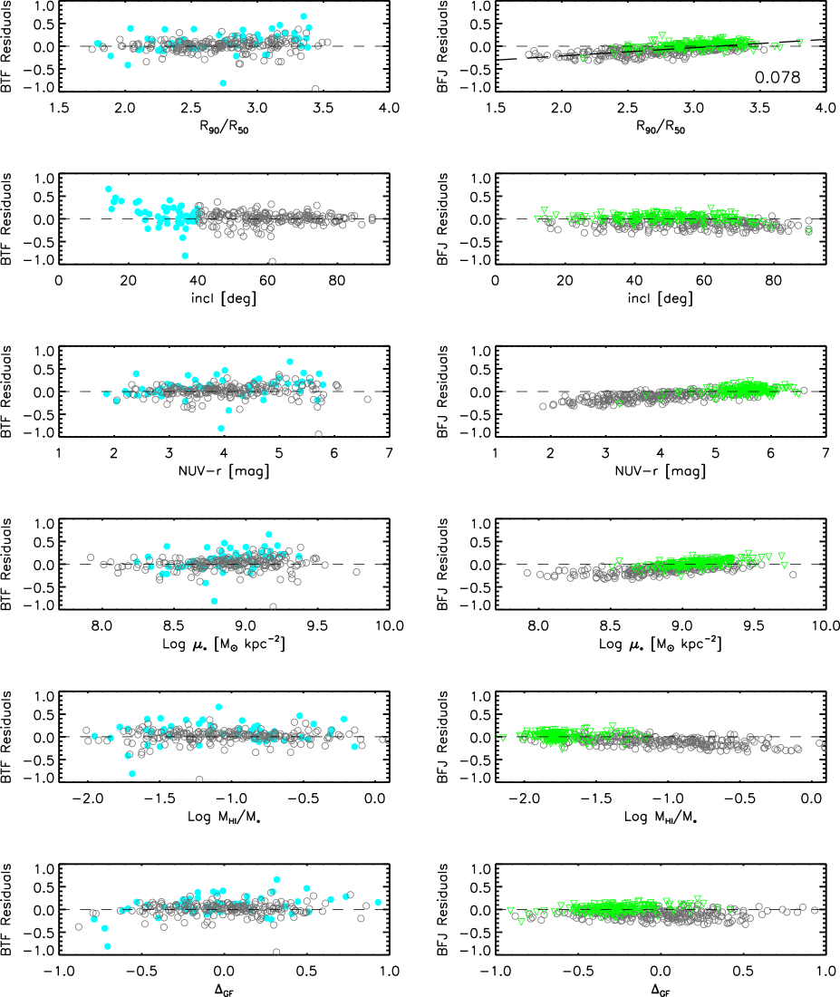
We now investigate how the residuals of the BTF relation depend on a few representative galaxy parameters. The left column of Figure 3 shows the BTF residuals for the sample in Figure 2a with respect to the best inverse fit obtained for the TF subset in Figure 2b. In other words, residuals are computed as , where is the measured rotational velocity and is the value expected from our best BTF relation for a galaxy with the same baryonic mass. Cyan filled circles indicate objects with inclination smaller than 40∘. From top to bottom, residuals are plotted as functions of concentration index, inclination, NUV color, stellar mass surface density, gas fraction, and distance from the gas fraction plane mentioned above and described in Paper I (galaxies more Hi-rich than the average have positive distance), respectively. BTF residuals do not exhibit strong dependence on structural and star-forming galaxy properties, except for a mild tendency toward increased scatter for more bulge-dominated, red galaxies, which largely disappears when the systems with low inclinations are removed from the sample. This is not surprising, as many attempts to identify a third parameter to minimize the scatter of the TF relation produced negative results (e.g., Courteau & Rix, 1999; Pizagno et al., 2007; Meyer et al., 2008, and references therein).
The results presented in this section show that the BTF is not very promising for our purpose of determining a relation between baryonic and dynamical mass that holds for all massive galaxies. Firstly, its application is restricted to galaxies with Hi detections and inclinations larger than 40∘. Secondly, the bulge-dominated systems with Hi detections are not simply offset from the relation defined by the disk-dominated galaxies, but are also more scattered. As demonstrated in the following two sections, the BFJ relation does not suffer from these limitations, and can be generalized to include both disk-dominated and spheroidal systems.
3.2 Baryonic Faber-Jackson Relation
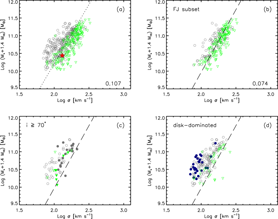
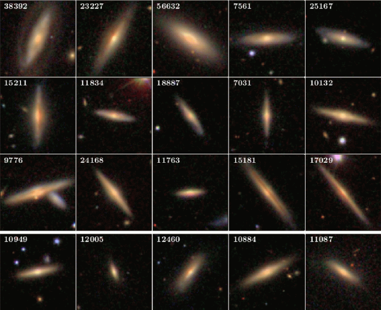
We now carry out a similar analysis for the BFJ relation. Since all the galaxies have a measurement of the stellar velocity dispersion from SDSS, we can use here the full sample, but it is instructive to keep Hi detections and non-detections separated. In Figure 4 the baryonic mass is plotted as a function of the stellar velocity dispersion, and green upside-down triangles indicate galaxies that were not detected with Arecibo. The relation plotted for the full GASS sample (panel a) shows a clear segregation between Hi detections and non-detections, the former being offset towards lower values of velocity dispersion. The gas-rich elliptical GASS 3505 (red star) is not unusual in terms of its stellar dispersion (GASS 35981 is not plotted because it has km s-1). We recover a tighter relation when we restrict our sample to the FJ subset (panel b), which includes bulge-dominated galaxies (i.e., objects with ) with inclinations smaller than 70∘. We excluded from the subset highly flattened systems because these are likely to host a significant disk component, despite their high concentration index. The 26 bulge-dominated galaxies excluded by our inclination cut are shown as filled symbols in Figure 4c. These are mostly Hi detections, which already suggests that they are more likely to be disks than oblate spheroids. Their SDSS images (Figure 5) confirm that they are inclined disks, often with dust lanes running along their major axis. As demonstrated by the bottom panels of Figure 4, disk-dominated galaxies are systematically offset from the best fit relation obtained for the data points in panel (b), and they are mostly Hi detections. These objects have low stellar velocity dispersions for fixed baryonic mass, thus they increase the scatter of the FJ relation when they are plotted together with the bulge-dominated galaxies.
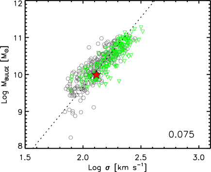
Because FJ studies usually do not include the gas component, we check our results by considering the stellar FJ relation. In particular, we compared our FJ relation with the one obtained for a large sample of SDSS galaxies by Gallazzi et al. (2006), which is conveniently expressed in terms of stellar masses. The slope and scatter of our FJ relation (restricted to the FJ subset) are in remarkable agreement with those published by Gallazzi et al. (2006) (both relations have a scatter of 0.071 dex), whereas the zero points differ by 0.17 dex in solar masses. The Gallazzi et al. (2006) sample includes galaxies with concentration index , redshift , and whose SDSS spectra have a median signal-to-noise per pixel greater than 20. Removing our inclination cut does not bring the zero points of the two relations into agreement (the offset is still 0.14 dex). However, Gallazzi et al. (2005) note that their stellar masses are systematically larger than those derived by Kauffmann et al. (2003) (and adopted here) by 0.1 dex, thus our results are completely consistent. Lastly, we notice that adding the gas to the stellar mass slightly increases the scatter of the relation (from 0.071 dex for the FJ to 0.074 dex for the BFJ). This is because the most Hi-rich galaxies in our sample (see for instance the blue points in Fig. 4d) become even further displaced from the Hi non-detections, which constitute the bulk of the FJ subset. A relation with similar scatter is obtained when, instead of restricting the sample to bulge-dominated systems, we consider only the bulge component itself. The mass of the bulge can be estimated from the correlation between SDSS concentration index and bulge-to-total stellar mass ratio, B/T, presented by Weinmann et al. (2009, see their Fig. 1), which is based on the 2D multicomponent decomposition analysis of Gadotti (2009). Our bilinear fit to their data yields B/T=(1.920)/2.276. The relation between bulge mass and stellar velocity dispersion plotted in Figure 6 has a scatter of 0.075 dex in velocity, comparable to that of the FJ and BFJ relations applied to the FJ subset (see also Gadotti & Kauffmann, 2009). Incidentally, it is somewhat surprising that we can recover such a tight relation given the uncertainties in our crude B/T estimate.
We now focus again on the baryonic FJ relation presented in Figure 4 and study its residuals. The BFJ residuals are plotted as functions of , inclination, NUV color, stellar mass surface density, gas fraction and distance from gas fraction plane on the right column of Figure 3. As for the BTF, these are the residuals for the sample in Figure 4a with respect to the best fit relation in Figure 4b, computed as described in § 3.1 (where is now stellar velocity dispersion). As in all the figures in this paper, green upside-down triangles indicate Hi non-detections. Interestingly, BFJ residuals show clear trends with concentration index, NUV color, , and gas fraction, in the sense that more disky, gas-rich and star-forming galaxies have larger residuals. A similar trend is seen as a function of Dn4000 index, which is an indicator of the age of the stellar population sampled by the SDSS 3″-diameter fiber (larger residuals are seen for smaller values of Dn4000, not shown). It is well known that the FJ relation for elliptical galaxies is a projection of a more general Fundamental Plane (Djorgovski & Davis, 1987; Dressler et al., 1987), which is usually parametrized in terms of stellar velocity dispersion, effective radius , and luminosity or surface brightness (central, or average within ). Thus, one might expect to see a dependence of the FJ residuals on a third parameter related to . However, the trends in Figure 3 are not a consequence of the Fundamental Plane. Firstly, our sample does not include only elliptical galaxies and spheroids. As can be seen by inspecting Figure 3, the trends are driven by the disk-dominated, star-forming galaxies. Secondly, quantities such as , NUV color or gas fraction are not directly related to an effective radius.
The comparison of the BTF and BFJ relations for our sample of massive galaxies illustrates several important points: (a) the BFJ is significantly less scattered than the BTF when the relations are applied to their maximum sample. When the two relations are applied to their respective “good”, morphologically-pruned subsets, the scatter in both is almost identical. (b) the BFJ is insensitive to the inclination problems that plague the BTF, which can be applied only to systems with inclination larger than 40∘. Furthermore, stellar dispersions are measured also for galaxies without Hi detections. Naturally, one could measure rotational velocities with other tracers and methods, e.g., with rotation curves. However, these have their own sets of problems (for instance, emission is typically significantly less extended than Hi emission, thus it may not trace the full rotational velocity. Moreover, it is unclear at which spatial position the rotational velocity should be measured. See, e.g., Catinella et al. 2007), and the inclination issue remains. (c) Most importantly, and contrary to the BTF case, the BFJ residuals show systematic trends with other galaxy properties. As shown in Figures 3 and 4, disk-dominated galaxies do not form a scatter plot in the BFJ plane, but they systematically deviate from the main relation defined by the bulge-dominated systems.
One might wonder if, for disk-dominated, inclined galaxies, is strongly affected by rotation. In other words, the BFJ for highly inclined disks (Figure 4c and 4d) could just be a TF relation in disguise. From the average rotation curves of disk galaxies of Catinella et al. (2006), we estimated that the typical rotational velocity reached at 1.5″ by GASS objects is 100 km s-1 (but could be up to twice as large for the most luminous and/or most distant galaxies in our sample)333 We converted SDSS model magnitudes into Cousins magnitudes following Catinella et al. (2008), and adopted , the radius containing 90% of the Petrosian flux in the SDSS -band, as a proxy for the optical radius , which is the radius encompassing 83% of the total I-band light of the galaxy. The average I-band absolute magnitude for our sample is 22.35 mag, and the average coverage of the SDSS fiber radius is 14% . . However, this does not take inclination and bulge-to-disk ratio within the aperture into account. Most importantly, the fiber measurements are intensity-weighted, thus most of the disk stars contributing to the dispersion are those closer to the galaxy center, where is negligible. Thus we conclude that measurements are not significantly affected by contamination from disk stars in circular orbits.
In summary, the SDSS stellar velocity dispersions provide an estimate of dynamical mass that — at least in the stellar mass and redshift regime probed by GASS — is not only more generally applicable (i.e., not limited to inclined galaxies with Hi detections or with extended rotation curves), but also less affected by measurement problems (which are largely responsible for the BTF outliers) compared to . Moreover, the fact that the disk-dominated galaxies follow a BFJ relation that is simply offset from that of the bulge-dominated systems suggests a simple way of bringing the two onto the same relation. This is accomplished in the next section.
3.3 A Generalized Baryonic Faber-Jackson Relation for All Massive Galaxies
Spheroids and disk-dominated galaxies can be brought onto the same BFJ-like relation by correcting the velocity dispersions for the trends observed in Figure 3. The tightest dependencies of the BFJ residuals are seen as a function of NUV color and concentration index. Although the correlation with NUV is slightly tighter (the dispersion of the linear fit is 0.073 dex), we decided to correct for the dependence on , which is a galaxy structural parameter. In fact, it is reasonable to expect larger corrections for more disk-dominated objects, where rotation is likely to be the main contributor to dynamical support. On the other hand, NUV color is linked to the star formation properties of the galaxy, thus the rationale for correcting velocity dispersions based on this quantity is much less evident. Moreover, a correction based on NUV has the additional disadvantage of requiring UV photometry.
The best linear fit to the data points in the top right panel of Figure 3 is:
| (4) |
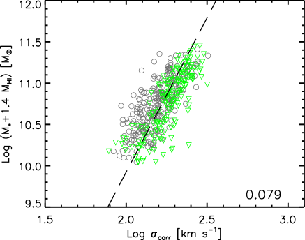
where the residuals are computed with respect to the best fit BFJ relation in Figure 4b. We thus corrected the velocity dispersions of all the galaxies in our sample by subtracting the offset . The BFJ relation obtained using the corrected velocity dispersions is plotted in Figure 7. The inverse fit is almost indistinguishable from that of Figure 4b, and has a scatter of 0.079 dex (the scatter in solar masses, obtained from a direct fit, is 0.218 dex). This relation holds for all the galaxies in our sample, regardless of morphology, inclination or gas content, and is the main result of this work.
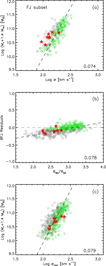
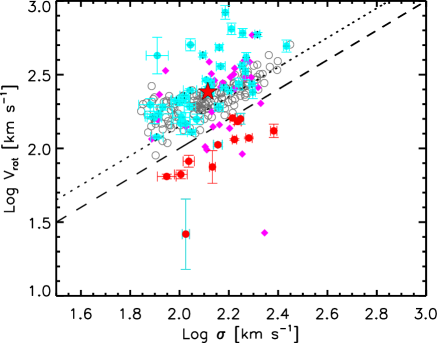
We compared our results with the simulations performed by Scannapieco et al. (2009, 2011), which follow the formation of eight Milky Way-mass halos in a -cold dark matter cosmology, including baryonic physics (star formation, metal cooling, chemical enrichment, multiphase gas, thermal feedback from supernovae). For these simulated galaxies we can measure stellar and cold gas masses, and stellar velocity dispersions at a given radius, and calculate concentration indices (from the ratio of the radii enclosing 90% and 50% of the total luminosity; we used r-band luminosities computed from the dust-free Bruzual & Charlot 2003 population synthesis models). We estimate total masses and luminosities within 10 kpc (the mean value of for the galaxies in the GASS sample), and obtain luminosity-weighted stellar velocity dispersions within 1.5 kpc (the physical size subtended by a 1.5″ radius at z=0.05). Using the concentration indices, we correct the stellar dispersions according to Equation 4. The results are illustrated in Figure 8, where we compare the positions of the simulated galaxies (red stars) with those of the FJ subset on the BFJ plane (a). The residuals from the BFJ fit are plotted as a function of in (b), and the generalized BFJ relation is shown in (c). The simulated galaxies are all disk-dominated according to our definition (i.e., ) except one, and their stellar dispersions are systematically offset from the fit in (a) towards smaller values, as the disk galaxies in the GASS sample are. The correction applied to their stellar dispersions removes the offset, and the simulated galaxies lie on top of the relation in (c). Although it is based on eight halos only, the excellent agreement between simulations and data is encouraging.
We have shown that disk-dominated galaxies are offset in the BFJ plane, and that this is what allow us to obtain a tight baryonic mass-velocity relation that holds for all the galaxies in our sample. The reason why there is a disk BFJ relation for massive galaxies is that is proportional to , and their ratio is a function of galaxy morphology. As demonstrated by Courteau et al. (2007b), for a given , earlier type galaxies have higher . The brightest, bulge-dominated galaxies (ellipticals, lenticulars and early-type spirals) lie on the relation expected for isothermal stellar systems. Later-type spiral and dwarf galaxies, on the other hand, depart from the isothermal relation by an amount that depends on morphology or total light concentration (see their Fig. 1). We plot the relation between and for the Hi-detected GASS galaxies in Figure 9. Our sample shows two populations of outliers, characterized by too large or too low ratios compared to the rest of the data set. These are the same outliers of the BTF relation (see Fig. 2); in particular, galaxies with large ratios all have small inclinations (∘, cyan), and objects with (red) were mentioned in § 3.1 and are discussed in the Appendix. To avoid crowding, we show error bars for these galaxies only444 The errors on rotational velocities are obtained from standard error propagation, taking into account the uncertainties in the observed velocity width and inclination (i.e., axis ratio in Eq. 1) only. The errors on stellar velocity dispersions are from the SDSS (as noted in § 2.2 the aperture correction is very small, thus we do not propagate its uncertainty). . Disregarding the outliers, one can see that the galaxies with larger stellar dispersions lie very close to the isothermal relation (indicated by a dotted line), whereas there is a tail of galaxies with higher ratios at lower dispersions. The galaxies in this tail are all disk dominated. Correcting the stellar dispersions according to Equation 4 effectively translates into accounting for this departure from isothermality for disk-dominated galaxies.
3.4 Empirical Baryonic Mass - Relation
In the previous section, we obtained a relation between baryonic mass and a measure of internal velocity that holds for our sample of massive galaxies, without any morphological pruning. We now ask whether we can find an even tighter relation by combining and measurements. Both quantities measure the depth of the gravitational potential well of a galaxy, but they do so at different radii, namely those of the bulge and of the outer disk (as traced by the Hi gas, which typically extends well beyond the stellar disk; however in very high-density environments Hi could be severely stripped; e.g., Giovanelli & Haynes 1985). In principle, Hi widths should provide the best measurement of the total mass (including dark) of a galaxy, regardless of the presence of a bulge component. However, as discussed above, reliable measurements are not possible for galaxies with small inclination to the line-of-sight — in the limit of a perfectly face-on system, which has no measurable rotation, the velocity dispersion of the stellar component is a more useful quantity. Thus, we have two methods of estimating the dynamical mass of a galaxy that are affected by different systematics and limitations. Can we combine them in order to obtain a quantity that is, on average, more tightly correlated with the baryonic mass? An interesting quantity in this context is the parameter (e.g., Covington et al., 2010):
| (5) |
This expression has been used in several studies, with different meanings for the dispersion component. Kassin et al. (2007) studied the TF relation for an emission line-selected sample of 544 galaxies at , and demonstrated that a remarkably tighter relation is obtained when the parameter is adopted instead of the rotational velocity from the optical rotation curve. In their case, is the dispersion of the gas (but this may be contaminated by velocity gradients, see their section 4.2). Interestingly, their sample includes early to late spirals, irregular galaxies and merging systems, and their -stellar mass relation for the lowest redshift bin is in very good agreement with the FJ relation of Gallazzi et al. (2006) in terms of slope and zero point.
More relevant for our work, Zaritsky et al. (2008) used the parameter (which they refer to as internal velocity, ) with measuring the stellar velocity dispersion of spheroidal galaxies. They showed that all classes of galaxies lie on a two-dimensional surface, which is expressed as a linear combination of the logarithms of the effective radius , the internal velocity squared, the surface brightness within , and the mass-to-light ratio within . Their sample is a heterogeneous collection of 1925 spheroids and disk galaxies from existing data sets, which span the full range of galaxy types and luminosities. However, although they define , they use either the circular velocity for disk galaxies or the stellar velocity dispersion for spheroids, but never add the two contributions.
Another interesting analysis was carried out by Covington et al. (2010), who studied the evolution of the stellar mass TF relation in a simulation of a disk merger. They argue that, since early-type galaxies are generally assumed to form through mergers of late-type systems, the scaling relations of early types should descend from those of late-type galaxies. Thus, they simulate the evolution of a galaxy merger, mimic observations of emission lines, and study how the kinematics of the system changes with time. The progenitors are two identical Sbc galaxies lying on the stellar mass TF relation, which merge and form a rotating elliptical galaxy. Intriguingly, they show that, while rotation is converted into stellar dispersion, the parameter is approximately conserved — suggesting that might be really tracing the mass distribution.
The above studies motivated us to look at the relation between baryonic mass and parameter for the galaxies in our sample, with an important caveat. The parameter defined by equation 5 has a physical meaning only if rotation and dispersion are associated to the same system. For instance, for a rotating isothermal sphere the dynamical support is provided by both ordered and thermal motions, and the above combination is a direct result of the virial theorem. For our galaxies, measures the rotational velocity of the gas, and is the velocity dispersion of the stars in the bulge, thus combining the two has no physical motivation. However, we are not trying to partition the dynamical support of a galaxy between its bulge and disk components — as we already pointed out, should account for the full dynamical support, regardless of the presence of a bulge. We wish instead to establish if we can average two measures of the potential well of a galaxy, which are based on different tracers, in order to obtain a quantity that, empirically, better correlates with the baryonic mass. After all, we expect the Hi width to be a more reliable measurement for inclined disk galaxies, and to be better for elliptical or face-on, disk galaxies. Thus, the combination of the two might work better on average.
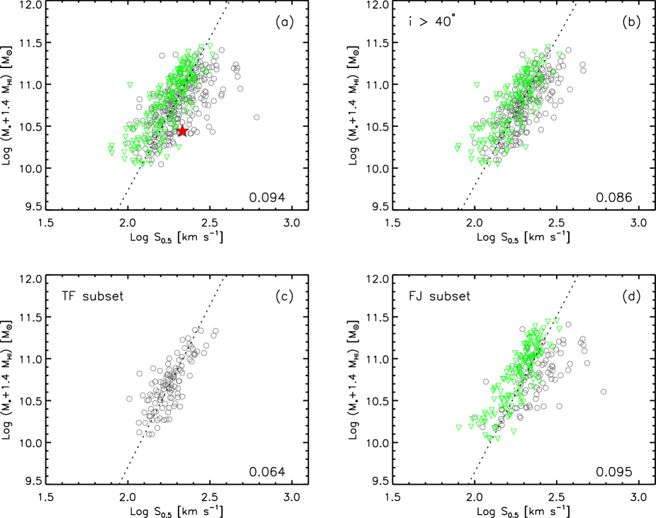
The correlation between baryonic mass and parameter is plotted in Figure 10 for the full sample (a), for the galaxies with inclinations larger than 40∘ (b), and for the TF and FJ subsets (c, d) defined in § 3.1 and § 3.2. The relation for the full sample has a scatter of 0.094 dex, very close to that of the BFJ relation for the full sample, but significantly larger than that of the generalized BFJ plotted in Figure 7. The relation still suffers from the inclination problems that affect the BTF, although to a lesser degree. The strongest outliers seen in Figure 10a are removed by our 40∘ inclination cut (b,c). Notice that, when applied to disk-dominated galaxies with inclinations larger than 40∘, the relation has a scatter of only 0.064 dex, i.e., it is tighter than the BTF shown in Figure 2b (which has a scatter of 0.076 dex) — this is in fact the tightest relation presented in this work (for comparison, the generalized BFJ relation restricted to the same sample has a scatter of 0.077 dex). Conversely, restricting the sample to bulge-dominated galaxies does not decrease the scatter of the relation. There is still a small offset between galaxies with and without Hi detections. Naturally, we do not have any information on the rotational velocity of the non-detections (some of which are disks close to edge-on view) — thus, for a fraction of these, is certainly underestimated. Overall, the baryonic relation is as good as our generalized BFJ, but only for galaxies with inclinations larger than 40∘.
4 Size-Velocity Relations
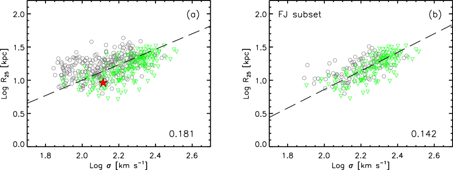
In this work we demonstrated that a simple correction applied to the stellar velocity dispersions removes the offset between disk-dominated galaxies and spheroids seen in the BFJ relation, i.e., to first order, it removes its dependence on the internal structure of the galaxy. We further investigate this by considering the size-velocity relation. The existence of such a correlation is well established for both disk galaxies (e.g., Courteau et al. 2007a; Avila-Reese et al. 2008; SS11 and references therein) and ellipticals or bulges of early-type spirals (the - relation, where is the diameter of the galaxy at a given surface brightness level; e.g., Dressler et al. 1987; Bernardi et al. 2002). Here, we compare this relation for the different velocity indicators and data subsets discussed in this work. Specifically, we wish to test how the correction to the stellar velocity dispersion introduced in § 3.3 affects the size-velocity relation.
The sizes of disk galaxies are commonly estimated from exponential scale lengths, . However, disk scale lengths are not only problematic to measure (e.g. Giovanelli et al. 1994; SS11), but are also not meaningful for elliptical galaxies. Saintonge et al. (2008) and SS11 advocate the use of isophotal radii instead of disk scale lengths, as they yield scaling relations with significantly lower scatter. Isophotal radii are also used as size indicators for early-type galaxies in the - relation. Thus, we adopt , which is half the 25 mag arcsec-2 isophote diameter measured by us on the SDSS g-band images, as a measure of size for all the galaxies in our sample. For comparison, varies between 2 and 7 , where is the SDSS exponential scale length in r-band, for the disk-dominated galaxies in our sample.
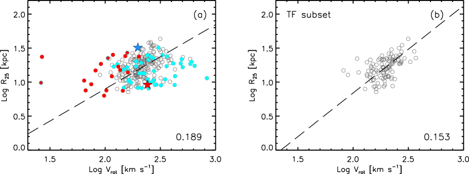
The relation between size and rotational velocity (RV) is shown in Figure 11a for all the galaxies with Hi detections. For this and the other relations presented in this section we performed bisector linear regressions instead of inverse fits, because it is less clear that the scatter is mostly confined to one variable. The scatter of about the best fit is computed as before, i.e., by applying Tukey’s bi-weight, and is noted in the bottom right corner of the plot (in dex of kpc). As in Figures 2 and 9, cyan and red circles indicate galaxies with inclinations smaller than 40∘ and with , respectively. Some of the main outliers of this relation are also outliers for the BTF, but there is not a 1-to-1 correspondence. For instance, the very Hi-rich spiral GASS 35981 (marked as a blue star) is an outlier on this plot, but not on the BTF, whereas the gas-rich elliptical GASS 3505 (red star) is an outlier for both relations.
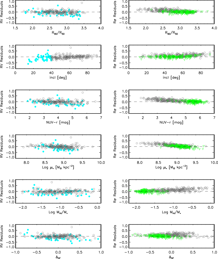
The RV relation is significantly weaker and more scattered than the BTF, as known from other studies that use disk scale lengths as size indicators (e.g., Courteau et al. 2007a report a Pearson correlation coefficient of and a scatter of 0.33 in log ). However, as mentioned above, SS11 obtain a very tight correlation using isophotal radii instead of disk scale lengths ( and a scatter of 0.11 in log R; in the notation adopted by these authors, the scatter of Courteau’s relation becomes 0.165 dex). When restricted to the TF subset (Fig. 11b), the scatter of our relation (0.15 dex) is intermediate between those of Courteau et al. (2007a) and SS11 samples. Although we use a similar size indicator as SS11, their sample includes only late-type spirals, thus the larger scatter of our relation is most likely due to the broader morphological mix of the galaxies in our data set. As for the BTF and BFJ relations, we plot the residuals of the RV relation as a function of several quantities in Figure 12 (left panels). There is a dependence of the RV residuals on inclination and, to a lesser extent, on .
Figure 13 shows the relation between and stellar velocity dispersion (R) for the full sample (a) and for the FJ subset (b). As for the BFJ relation, galaxies with Hi detections are displaced from the non-detections (green triangles), and a clear trend is observed when the R residuals are plotted as a function of concentration index (Fig. 12, top right panel). Indeed, Figure 12 shows that the R residuals behave similarly to the BFJ ones (see Fig. 3): disk-dominated galaxies systematically deviate from the best fit relation obtained for the FJ subset, which is dominated by spheroids. Aside from systematic trends, which are stronger for the R relation, the scatter of the RV and R relations is very similar, for both maximum samples and pruned subsets.
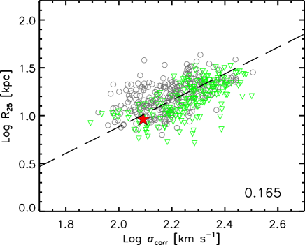
Lastly, correcting the velocity dispersions according to Equation 4 yields a slightly tighter size-velocity relation (Fig. 14). Most importantly, our correction removes the offset between Hi detections and non-detections present in Figure 13a (the remaining few Hi detections lying above the relation are highly inclined galaxies, for which , which is not corrected for inclination, is likely to be overestimated).
5 Discussion and Conclusions
The main result of this work is the existence of a tight relation between baryonic mass and velocity that is independent of galaxy morphology. To first order, we can remove the dependence of dynamical scaling relations on the internal structure of the galaxy by applying a simple correction to the measured stellar velocity dispersions, which depends only on the concentration index (Eq. 4). The correlation between baryonic mass and corrected thus obtained has a scatter of only 0.08 dex (Fig. 7 and Table 1). It is encouraging that our correction removes the offset between disks and spheroids also in the size-velocity relation (expressed in terms of versus stellar dispersion). We tested if an even tighter baryonic mass-velocity relation could be obtained by using the parameter, which combines rotational velocity and stellar dispersion. We found no improvement, because the relation still suffers from the problem of low inclination galaxies that affects the BTF, to a lesser extent. Despite being measured at a smaller spatial scale than the Hi width, the stellar velocity dispersion turns out to be a better tracer of mass, at least for the massive galaxies in our sample. This is surprising, as one would expect the rotational velocity to provide a more reliable measurement of mass for galaxies with Hi detections, the vast majority of which are rotation dominated (i.e., 216/228 galaxies have ), regardless of the presence of a bulge. And yet, the same result was obtained by Neistein et al. (1999) for a sample of S0 galaxies with inclinations 35∘60∘, which are also, overall, rotation-dominated: the central stellar velocity dispersion is a better predictor of I-band luminosity than the circular speed at 2-3 exponential disk scale lengths, which they carefully measured from long-slit optical absorption-line spectra.
As we already pointed out, the main limitation with rotational velocities is observational, not intrinsic. We are simply not able to reliably measure circular speeds from line-of-sight velocities, except for well-selected samples of undisturbed late-type, inclined spirals (i.e., the typical TF samples), for which the deprojection to edge-on view does not introduce very large uncertainties. As for the velocity dispersions, which are measured through 3″-diameter fibers, there might be a concern about contamination from disk stars in circular orbits, especially for the most edge-on, disk-dominated galaxies. However, we have argued that this effect is negligible (§ 3.2). This agrees with the conclusion reached by Courteau et al. (2007b), who reported that the contamination is small (, based on simulations) for Milky Way-type galaxies with pressure-supported bulges.
We argued that the reason why disk-dominated galaxies are simply offset from the spheroids on the BFJ plane (which is the key point that allows us to bring all massive galaxies onto the same baryonic mass-velocity relation) is that is proportional to , and their ratio is a function of galaxy morphology. Although initial work indicated that spirals and ellipticals follow the same tight - correlation for km s-1 (e.g., Ferrarese, 2002; Baes et al., 2003; Pizzella et al., 2005), more recent analyses demonstrate that the relation between and is not universal, but depends on morphology. As mentioned in § 3.3, Courteau et al. (2007b) show that the brightest, bulge-dominated galaxies lie on the relation expected for isothermal stellar systems, whereas later-type spirals and dwarfs are offset by an amount that depends on morphology or total light concentration. We have shown that correcting the stellar dispersions according to Equation 4 effectively translates into accounting for this departure from isothermality for disk-dominated galaxies. Courteau et al. (2007b) noted that, despite the fact that a detailed understanding of what sets the relation between , and concentration index is still missing, one could use this relation to empirically reduce the scatter of scaling relations that involve dynamical parameters, such as the TF or FJ. We showed that the existence of such relation allows us to do more than that — we obtained a generalized BFJ relation that holds for all the massive galaxies in our sample, with a scatter (0.079 dex) that is as small as that of the BTF and BFJ relations applied to their pruned subsets (i.e. 0.076 and 0.074 dex, respectively). For comparison, Avila-Reese et al. (2008) and Gallazzi et al. (2006) report a scatter of 0.06 dex for the BTF and 0.071 dex for the stellar FJ relations, respectively.
The implications of our generalized BFJ relation for extragalactic studies are very promising. Because it holds for all massive galaxies in our sample regardless of morphology, this relation appears to provide a more fundamental link between dark matter halo mass and baryonic content than that obtained using rotational velocities or velocity dispersions. As such, it gives more fundamental constraints to galaxy formation models than the TF or FJ/FP relations. Also this is the reference baryonic mass-internal velocity relation that higher redshift studies, which naturally target the most massive galaxies, should compare with. This relation is more resilient to systematic effects than the TF, and, contrary to both TF and FJ/FP relations, does not require any morphological pruning — a significant advantage since accurate morphological classifications are difficult to obtain for large samples beyond the very local Universe.
As pointed out throughout this work, our results are based on a representative sample of galaxies with stellar masses larger than M⊙. It remains to be established how far down in stellar mass these results can be extrapolated. It would be beneficial to investigate whether a BFJ relation for disk galaxies holds down to low baryonic masses (where the gas contribution is more important), and with similarly low scatter, based on a representative and homogeneous sample such as GASS.
Acknowledgments
B.C. wishes to thank Dennis Zaritsky, Susan Kassin, Thorsten Naab and Luca Cortese for useful discussions. Thanks also to Simone Weinmann for kindly providing the data on concentration index versus B/T ratio used in section 3.2.
The Arecibo Observatory is part of the National Astronomy and Ionosphere Center, which is operated by Cornell University under a cooperative agreement with the National Science Foundation.
GALEX (Galaxy Evolution Explorer) is a NASA Small Explorer, launched in April 2003. We gratefully acknowledge NASA’s support for construction, operation, and science analysis for the GALEX mission, developed in cooperation with the Centre National d’Etudes Spatiales (CNES) of France and the Korean Ministry of Science and Technology.
Funding for the SDSS and SDSS-II has been provided by the Alfred P. Sloan Foundation, the Participating Institutions, the National Science Foundation, the U.S. Department of Energy, the National Aeronautics and Space Administration, the Japanese Monbukagakusho, the Max Planck Society, and the Higher Education Funding Council for England. The SDSS Web Site is http://www.sdss.org/.
The SDSS is managed by the Astrophysical Research Consortium for the Participating Institutions. The Participating Institutions are the American Museum of Natural History, Astrophysical Institute Potsdam, University of Basel, University of Cambridge, Case Western Reserve University, University of Chicago, Drexel University, Fermilab, the Institute for Advanced Study, the Japan Participation Group, Johns Hopkins University, the Joint Institute for Nuclear Astrophysics, the Kavli Institute for Particle Astrophysics and Cosmology, the Korean Scientist Group, the Chinese Academy of Sciences (LAMOST), Los Alamos National Laboratory, the Max-Planck-Institute for Astronomy (MPIA), the Max-Planck-Institute for Astrophysics (MPA), New Mexico State University, Ohio State University, University of Pittsburgh, University of Portsmouth, Princeton University, the United States Naval Observatory, and the University of Washington.
Appendix: Galaxies with
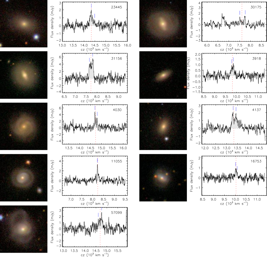
We discuss here in more detail the 12 galaxies with Hi rotational velocities smaller than their stellar velocity dispersions, which are outliers of both BTF and versus relations. These objects are indicated by red symbols in Figures 2 and 9. While the high outliers are all galaxies with small inclinations, for which the rotational velocities are likely to be overestimated, the low outliers are potentially more interesting. As mentioned in § 3.1, Ho (2007) identifies a population of galaxies with unusually small ratios, which are outliers in his TF relation, and argues that these systems must have experienced gas accretion. Figure 15 shows SDSS images and Hi-line profiles for 9 outliers detected by GASS (the other galaxies were either observed by ALFALFA or included in the S05 archive). Two of these galaxies, GASS 30175 and 31156, are outliers because their SDSS inclinations are incorrect. They both have strong bars which dominate the SDSS fits, thus overestimating the inclination (54∘ and 61∘ for GASS 30175 and 31156; we measured 37∘ and 27∘ respectively). The same is true for GASS 24236 (AGC 220363, detected by ALFALFA and not shown here), a nearly face-on barred galaxy with SDSS inclination of 46∘ (we measured 17∘). Of the remaining outliers, one is clearly morphologically disturbed (GASS 57099, bottom row). Another galaxy, GASS 4030, was observed as part of the COLDGASS survey (Saintonge et al., 2011, see their Figure A1, row 6). Its (uncorrected) velocity width measured from the CO(1-0) spectrum is 137 km s-1, which is exactly the same as the (uncorrected) Hi width. Since the CO(1-0) emission typically originates from the central regions of a galaxy, perhaps the fact that CO and Hi widths are identical means that the Hi gas in this galaxy is not extended enough to sample the flat part of the rotation curve. This is not particularly unusual, as there are other examples of early-type spirals with truncated Hi disks (e.g. NGC 3623, where the Hi emission does not extend beyond the stellar disk; Hogg et al. 2001) or unexpectedly narrow Hi profiles (e.g. NGC 5854; Haynes et al. 2000). Overall, even acknowledging that some of these profiles are not very high signal-to-noise detections, it is striking that most are asymmetric, suggesting disturbances in the distribution and/or kinematics of the Hi gas. We will investigate asymmetries of Hi profiles in more detail in a future work.
| Log = a Log +b[b] | |||||
|---|---|---|---|---|---|
| N[a] | a | b | scatter[c] | ||
| BTF, Hi detections | 259 | 0.250 | 0.365 | 0.127 | |
| BTF, TF subset | 108 | 0.237 | 0.251 | 0.076 | |
| BFJ | 436 | 0.299 | 1.053 | 0.107 | |
| BFJ, FJ subset | 231 | 0.283 | 0.818 | 0.074 | |
| Generalized BFJ | 436 | 0.267 | 0.654 | 0.079 | |
| Baryonic | 436 | 0.274 | 0.670 | 0.094 | |
| Baryonic , ∘ | 341 | 0.285 | 0.791 | 0.086 | |
[a]Number of galaxies in the sample.
[c]Scatter in dex of km s-1.
| Log = a Log +b[b] | |||||
|---|---|---|---|---|---|
| N[a] | a | b | scatter[c] | ||
| RV, Hi detections | 259 | 0.946 | 0.992 | 0.189 | |
| RV, TF subset | 108 | 1.284 | 1.728 | 0.153 | |
| R | 436 | 1.162 | 1.323 | 0.181 | |
| R, FJ subset | 231 | 1.399 | 1.937 | 0.142 | |
| R | 436 | 1.385 | 1.887 | 0.165 | |
[a]Number of galaxies in the sample.
[c]Scatter in dex of kpc.
References
- Abazajian et al. (2009) Abazajian, K. N. et al. 2009, ApJS, 182, 543
- Avila-Reese et al. (2008) Avila-Reese, V., Zavala, J., Firmani, C., & Hernández-Toledo, H. M. 2008, AJ, 136, 1340
- Baes et al. (2003) Baes, M., Buyle, P., Hau, G. K. T., & Dejonghe, H. 2003, MNRAS, 341, L44
- Baldry et al. (2006) Baldry, I. K., Balogh, M. L., Bower, R. G., Glazebrook, K., Nichol, R. C., Bamford, S. P., & Budavari, T. 2006, MNRAS, 373, 469
- Bedregal et al. (2006) Bedregal, A. G., Aragón-Salamanca, A., & Merrifield, M. R. 2006, MNRAS, 373, 1125
- Begum et al. (2008) Begum, A., Chengalur, J. N., Karachentsev, I. D., & Sharina, M. E. 2008, MNRAS, 386, 138
- Bernardi et al. (2002) Bernardi, M., Alonso, M. V., da Costa, L. N., Willmer, C. N. A., Wegner, G., Pellegrini, P. S., Rité, C., & Maia, M. A. G. 2002, AJ, 123, 2159
- Bernardi et al. (2003) Bernardi, M. et al. 2003, AJ, 125, 1817
- Bruzual & Charlot (2003) Bruzual, G., & Charlot, S. 2003, MNRAS, 344, 1000
- Catinella et al. (2006) Catinella, B., Giovanelli, R., & Haynes, M. P. 2006, ApJ, 640, 751
- Catinella et al. (2007) Catinella, B., Haynes, M. P., & Giovanelli, R. 2007, AJ, 134, 334
- Catinella et al. (2008) Catinella, B., Haynes, M. P., Giovanelli, R., Gardner, J. P., & Connolly, A. J. 2008, ApJ, 685, L13
- Catinella et al. (2010) Catinella, B., Schiminovich, D., Kauffmann, G. et al. 2010, MNRAS, 403, 683 (Paper I)
- Chabrier (2003) Chabrier, G. 2003, PASP, 115, 763
- Courteau (1997) Courteau, S. 1997, AJ, 114, 2402
- Courteau et al. (2003) Courteau, S., Andersen, D. R., Bershady, M. A., MacArthur, L. A., & Rix, H.-W. 2003, ApJ, 594, 208
- Courteau et al. (2007a) Courteau, S., Dutton, A. A., van den Bosch, F. C., MacArthur, L. A., Dekel, A., McIntosh, D. H., & Dale, D. A. 2007a, ApJ, 671, 203
- Courteau et al. (2007b) Courteau, S., McDonald, M., Widrow, L. M., & Holtzman, J. 2007b, ApJ, 655, L21
- Courteau & Rix (1999) Courteau, S. & Rix, H.-W. 1999, ApJ, 513, 561
- Courtois et al. (2009) Courtois, H. M., Tully, R. B., Fisher, J. R., Bonhomme, N., Zavodny, M., & Barnes, A. 2009, AJ, 138, 1938
- Covington et al. (2010) Covington, M. D. et al. 2010, ApJ, 710, 279
- De Rijcke et al. (2007) De Rijcke, S., Zeilinger, W. W., Hau G. K. T., Prugniel, P., & Dejonghe H., 2007, ApJ, 659, 1172
- Djorgovski & Davis (1987) Djorgovski, S. & Davis, M. 1987, ApJ, 313, 59
- Dressler et al. (1987) Dressler, A. 1987, ApJ, 317, 1
- Dressler et al. (1987) Dressler, A., Lynden-Bell, D., Burstein, D., Davies, R. L., Faber, S. M., Terlevich, R., & Wegner, G. 1987, ApJ, 313, 42
- Driver et al. (2007) Driver, S. P., Allen, P. D., Liske, J., & Graham, A. W. 2007, ApJ, 657, L85
- Dutton et al. (2007) Dutton, A. A., van den Bosch, F. C., Dekel, A., & Courteau, S. 2007, ApJ, 654, 27
- Faber & Jackson (1976) Faber, S. M. & Jackson, R. E. 1976, ApJ, 204, 668
- Ferrarese (2002) Ferrarese, L. 2002, ApJ, 578, 90
- Gadotti (2009) Gadotti, D. A. 2009, MNRAS, 393, 1531
- Gadotti & Kauffmann (2009) Gadotti, D. A. & Kauffmann, G. 2009, MNRAS, 399, 621
- Gallazzi et al. (2005) Gallazzi, A., Charlot, S., Brinchmann, J., White, S. D. M. & Tremonti, C. A. 2005, MNRAS, 362, 41
- Gallazzi et al. (2006) Gallazzi, A., Charlot, S., Brinchmann, J., & White, S. D. M. 2006, MNRAS, 370, 1106
- Geha et al. (2006) Geha, M., Blanton, M., Masjedi, M., & West, A. 2006, ApJ, 653, 240
- Giovanelli et al. (1997a) Giovanelli, R., Haynes, M. P., Herter, T., Vogt, N. P., Wegner, G. Salzer, J. J., da Costa, L. N., & Freudling, W. 1997a, AJ, 113, 22
- Giovanelli et al. (1997b) Giovanelli, R., Haynes, M. P., Herter, T., Vogt, N. P., da Costa, L. N., Freudling, W., Salzer, J. J., & Wegner, G. 1997b, AJ, 113, 53
- Giovanelli et al. (1994) Giovanelli, R., Haynes, M. P., Salzer, J. J., Wegner, G., da Costa, L. N., & Freudling, W. 1994, AJ, 107, 2036
- Giovanelli et al. (2005) Giovanelli, R. et al. 2005, AJ, 130, 2598
- Giovanelli & Haynes (1985) Giovanelli, R. & Haynes, M. P. 1985, ApJ, 292, 404
- Graves et al. (2009) Graves, G. J., Faber, S. M., & Schiavon, R. P. 2009, ApJ, 693, 486
- Gurovich et al. (2010) Gurovich, S., Freeman, K. C., Jerjen, H., Staveley-Smith, L., & Puerari, I. 2010, AJ, 140, 663
- Gurovich et al. (2004) Gurovich, S., McGaugh, S. S., Freeman, K. C., Jerjen, H., Staveley-Smith, L., & De Blok, W. J. G. 2004, PASA, 21, 412
- Haynes et al. (2000) Haynes, M. P., Jore, K. P., Barrett, E. A., Broeils, A. H., & Murray, B. M. 2000, AJ, 120, 703
- Ho (2007) Ho, L. C. 2007, ApJ, 668, 94
- Hogg et al. (2001) Hogg, D. E., Roberts, M. S., Bregman, J. N., & Haynes, M. P. 2001, AJ, 121, 1336
- Holmberg (1958) Holmberg, E. 1958, Lund Medd. Astron. Obs. Ser. II, 136, 1
- Iodice et al. (2003) Iodice, E., Arnaboldi, M., Bournaud, F., Combes, F., Sparke, L. S., van Driel, W., & Capaccioli, M. 2003, ApJ, 585, 730
- Kannappan et al. (2002) Kannappan, S. J., Fabricant, D. G., & Franx, M. 2002, AJ, 123, 2358
- Kassin et al. (2007) Kassin, S. A. et al. 2007, ApJ, 660, L35
- Kauffmann et al. (2003) Kauffmann, G. et al. 2003, MNRAS, 341, 33
- Kent et al. (2008) Kent, B. R. et al. 2008, AJ, 136, 713
- Martin et al. (2005) Martin, D. C. et al. 2005, ApJ, 619, L1
- Masters et al. (2006) Masters, K. L., Springob, C. M., Haynes, M. P., & Giovanelli, R. 2006, ApJ, 653, 861
- McGaugh (2005) McGaugh, S. S. 2005, ApJ, 632, 859
- McGaugh et al. (2000) McGaugh, S. S., Schombert, J. M., Bothun, G. D., & de Blok, W. J. G. 2000, ApJ, 533, L99
- Meyer et al. (2008) Meyer, M. J., Zwaan, M. A., Webster, R. L., Schneider, S., & Staveley-Smith, L. 2008, MNRAS, 391, 1712
- Mo et al. (1998) Mo, H. J., Mao, S., & White, S. D. M. 1998, MNRAS, 295, 319
- Moran et al. (2010) Moran, S. M. et al, 2010, ApJ, 720, 1126
- Neistein et al. (1999) Neistein, E., Maoz, D., Rix, H.-W., & Tonry, J. L. 1999, AJ, 117, 2666
- Noordermeer & Verheijen (2007) Noordermeer, E., & Verheijen, M. A. W. 2007, MNRAS, 381, 1463
- Paturel et al. (2003a) Paturel, G., Petit, C., Prugniel, P., Theureau, G., Rousseau, J., Brouty, M., Dubois, P., & Cambrésy, L. 2003a, A&A, 412, 45
- Paturel et al. (2003b) Paturel, G., Theureau, G., Bottinelli, L., Gouguenheim, L., Coudreau-Durand, N., Hallet, N., & Petit, C. 2003b, A&A, 412, 57
- Pizagno et al. (2007) Pizagno, J. et al. 2007, AJ, 134, 945
- Pizzella et al. (2005) Pizzella, A., Corsini, E. M., Dalla Bontà, E., Sarzi, M., Coccato, L., & Bertola, F. 2005, ApJ, 631, 785
- Saintonge et al. (2008) Saintonge, A., Masters, K. L., Marinoni, C., Spekkens, K., Giovanelli, R., & Haynes, M. P. 2008, A&A, 478, 57
- Saintonge & Spekkens (2011) Saintonge, A., & Spekkens, K. 2011, ApJ, 726, 77 (SS11)
- Saintonge et al. (2011) Saintonge, A. et al. 2011, MNRAS, 415, 32
- Salim et al. (2007) Salim, S. et al. 2007, ApJS, 173, 267
- Scannapieco et al. (2009) Scannapieco, C., White, S. D. M, Springel, V., & Tissera, P. B. 2009, MNRAS, 396, 696
- Scannapieco et al. (2011) Scannapieco, C., White, S. D. M, Springel, V., & Tissera, P. B. 2011, arXiv:1105.0680
- Springob et al. (2005) Springob, C. M., Haynes, M. P., Giovanelli, R., & Kent, B. R. 2005, ApJS, 160, 149 (S05)
- Tully & Fisher (1977) Tully, R. B. & Fisher, J. R. 1977, A&A, 54, 661
- Tully et al. (2009) Tully, R. B., Rizzi, L., Shaya, E. J., Courtois, H. M., Makarov, D. I., & Jacobs, B. A. 2009, AJ, 138, 323
- Wang et al. (2011) Wang, J. et al. 2011, MNRAS, 412, 1081
- Weinmann et al. (2009) Weinmann, S. M., Kauffmann, G., van der Bosch, F. C., Pasquali, A., McIntosh, D. H., Mo, H., Yang, X., & Guo, Y. 2009, MNRAS, 394, 1213
- Williams et al. (2010) Williams, M. J., Bureau, M., & Cappellari, M. 2010, MNRAS, 409, 1330
- York et al. (2000) York, D. G., et al. 2000, AJ, 120, 1579
- Zaritsky et al. (2008) Zaritsky, D., Zabludoff, A. I., & Gonzalez, A. H. 2008, ApJ, 682, 68