Dust processing in Supernova Remnants: Spitzer MIPS SED and IRS Observations

Abstract

We present Spitzer MIPS SED and IRS observations of 14 Galactic Supernova Remnants previously identified in the GLIMPSE survey. We find evidence for SNR/molecular cloud interaction through detection of [O I] emission, ionic lines, and emission from molecular hydrogen. Through black-body fitting of the MIPS SEDs we find the large grains to be warm, 29–66 K. The dust emission is modeled using the DUSTEM code and a three component dust model composed of populations of big grains, very small grains, and polycyclic aromatic hydrocarbons. We find the dust to be moderately heated, typically by 30–100 times the interstellar radiation field. The source of the radiation is likely hydrogen recombination, where the excitation of hydrogen occurred in the shock front. The ratio of very small grains to big grains is found for most of the molecular interacting SNRs to be higher than that found in the plane of the Milky Way, typically by a factor of 2–3. We suggest that dust shattering is responsible for the relative over-abundance of small grains, in agreement with prediction from dust destruction models. However, two of the SNRs are best fit with a very low abundance of carbon grains to silicate grains and with a very high radiation field. A likely reason for the low abundance of small carbon grains is sputtering. We find evidence for silicate emission at 20 $\mu$m in their SEDs, indicating that they are young SNRs based on the strong radiation field necessary to reproduce the observed SEDs.

1 Introduction

Supernovae have a profound effect on their environment. Supernova remnants (SNRs) will compress and heat the surrounding interstellar material and potentially alter its chemical composition. Due to the short life time of massive stars, it is expected that a significant fraction of massive stars will explode as supernovae in or nearby molecular clouds. However, until recently, only a few SNRs are known interacting with a surrounding molecular cloud.

Using Spitzer GLIMPSE survey data (Churchwell et al., 2009), Reach et al. (2006) identified a series of Galactic SNRs in the infrared, a sub-sample having IRAC colors that could indicate emission from shocked H₂. The analysis of follow-up Spitzer IRS low resolution spectra confirmed the detection of H₂ in all of the SNRs (6 from Hewitt et al. (2009) and the rest in this paper), more than doubling the sample of known interacting Galactic SNRs.

Interacting SNRs are an ideal laboratory to study the effects of fast shocks on the interstellar material. A series of papers have predicted that shocks can both sputter and shatter the interstellar dust and thus potentially modify its abundance and size distribution (e.g. Borkowski & Dwek, 1995; Jones et al., 1994; Guillet et al., 2007, 2009). Changes in the dust distribution and abundance will impact the extinction law of the dust and SNRs are a unique possibility to observationally constrain the shock models.

Previous observations of interacting SNRs are limited. Since they are located in the Galactic plane, there is a significant contribution from unrelated material along the line of sight. Previous studies, utilizing mainly ISO observations, of e.g. 3C391, W28, and W44 had to rely on a fit to the general Galactic background emission to obtain the emission from the SNR. ISO observations of 3C391 found that $\sim$1 M_⊙ of shock excited dust was present within the 80 arcseconds FWHM beam (Reach & Rho, 2000). Conversely, the Si and Fe lines in the spectra indicated a total amount of vaporized dust of 0.5 M_⊙, suggesting a dust destruction of $\sim$30% in 3C391. For W28, and W44, the dust emission from the SNR was relatively weak compared to the Galactic emission and the dust mass could not be constrained. Because of improved background subtraction which has been possible with Spitzer data due to the spatial coverage of the slit, the additional uncertainty from the background modeling can be reduced.

The dust analysis of interacting SNRs using ISO data described above was limited to long wavelengths (greater than 40 $\mu$m). Shorter wavelength observations are necessary to probe the emission from the very small grains and polycyclic aromatic hydrocarbons (PAHs) in greater details. The ratio of the very small grain (VSG) to big grain (BG) abundances can provide insight into dust destruction mechanisms. Dust destruction models predict a different destruction efficiency for graphite and silicates, respectively (e.g. Jones et al., 1994). The models further predicts a strong dependence on grain size for the dust destruction efficiency. Thus, a comparison of the ratio of VSGs to BGs in the SNRs with the similar ratio determined in the Galaxy and the LMC (e.g. Bernard et al., 2008) will provide constraints on dust destruction models.

Here we present an analysis of the continuum and PAH emission as well as the [O I] 63 $\mu$m emission from a sample of inner Galaxy SNRs. We discuss MIPS SED observations and low resolution IRS spectra of a sample of 14 SNRs. The observations were centered on the emission peaks for each SNR identified in the GLIMPSE data (Reach et al., 2006). The wavelength coverage from 5 to 80 $\mu$m ensures a good sampling of the three main dust species and enables us to fit the continuum in greater detail than previous mid–infrared observations that had much lower spatial resolution and lacked proper background subtraction.

The paper is structured as follows. In Section 2 we present the observations and describe the data reduction. We outline the basic results in Section 3. Modified black bodies are fitted to the long wavelength data and used to estimate the temperature of the big grains. We further discuss the detection of the [O I] line at 63 $\mu$m in several of the MIPS SEDs. We fit the continuum with a three-component dust model and discuss the basic properties for each SNR in Section 4. In Section 5 we discuss the derived relative abundance of the dust species. The total amount of dust in each SNR is then estimated from the 24 and 70 $\mu$m image by extrapolation of the results of the dust fitting to the whole SNR. Finally, we present our conclusions in Section 6.

2 Observations

We have obtained Spitzer MIPS SED observations and IRS low resolution spectra of a total of 14 individual Galactic SNRs as part of cycle 3 (program ID 30585; PI: J. Rho). Three of the SNRs, CTB37A, RCW103, and 3C396 were observed at two positions. For all 17 positions we have obtained low–resolution (LR) IRS spectra in all four sub–slits of the LR module, covering the 5–35 $\mu$m range as well as MIPS SEDs. Part of the IRS data were discussed in Hewitt et al. (2009). Here we present the line intensities for the remaining SNRs and discuss the continuum emission from the whole sample. The basic characteristics for a subset of the SNRs discussed in this paper were described in Hewitt et al. (2009). For the remaining SNRs, the data are summarized in Table 1 and the details are provided in Section 4.4. Below we describe the data reduction.

Table 1: Basic properties of sample SNRs^a

Name	Other name	RA	DEC	distance	Diameter	Size	NH
		(J2000)	(J2000)	(kpc)	(′)	(pc)	($10^{22}$cm-2)
G11.2-0.3	$\cdots$	18:11:32.3	-19:27:12	5.0	4	5.8	2.0
Kes69	G21.8-0.6	18:33:01.9	-10:13:43	5.2	20	30	2.4
G22.7-0.2	$\cdots$	18:33:09.0	-09:26:41	3.7	26	28	7.8
3C396cent	G39.2-0.3	19:04:18.7	+05:26:31	8.0	8x6	16	4.7
3C396shell	G39.2-0.3	19:03:56.2	+05:25:50	8.0	8x6	16	4.7
G54.4-0.3	$\cdots$	19:33:05.5	19:16:47	3.0	40	35	1.0
Kes17	G304.6+0.1	13:05:32.8	-62:40:06	9.7	8	23	3.6
Kes 20A	G310.8-0.4	14:00:41.4	-62:20:21	13.7	12	48	7.9
G311.5-0.3	$\cdots$	14:05:22.1	-61:58:11	14.8	5	21.5	2.5
RCW103	G332.4-0.4	16:17:31.8	-51:06:34	3.1	10	9	0.7
RCW103fill	G332.4-0.4	16:17:14.8	-51:01:40	3.1	10	9	0.7
G344.7-0.1	$\cdots$	17:03:57.6	-41:40:51	14.0	10	41	5.5
G346.6-0.2	$\cdots$	17:10:14.6	-40:14:38	11	8	26	2.7
G348.5-0.0	$\cdots$	17:15:04.9	-38:33:41	11.3	10	33	2.8
CTB 37A–N	G348.5+0.1	17:14:25.8	-38:33:09	11.0	15	48	3.2
CTB 37A–S	G348.5+0.1	17:14:35.0	-38:28:20	11.0	15	48	3.2
G349.7+0.2	$\cdots$	17:18:00.7	-37:26:16	22.4	2.5x2	15	5.8

2.1 MIPS SEDs

Mid–infrared observations of the SNRs were obtained using the SED mode of the MIPS instrument. The spectral dispersion is 1.771 $\mu$m pixel^-1 over the wavelength range 53$\mu$m to 96$\mu$m. Details for the MIPS SED mode can be found in Lu et al. (2008). Observations were obtained in a standard on–off pattern with an offset of 3′. Each cycle of on-off positions consisted of a STIM flash and 3 subsequent on–off pairs. For each SNR we obtained 10 cycles with the integration time chosen to be 3.15 seconds for each on and off position. We have adopted the pipeline processed BCD frames and produced the final on and off mosaics using the mopex software provided by the Spitzer Science Center. However, the flash associated with the STIM was found to contaminate the first on–off pair and these have been manually excluded before the data were co–added. The total integration time for the on and off positions is 63 seconds. The locations of the on and off positions are superposed on the images of the SNRs shown in Figure  1.

The location of the emission from the SNR within the slit was in each case identified through visual inspection and by comparison with the MIPSGAL images at both 24 $\mu$m and 70 $\mu$m. The spectrum was extracted over 3 pixels in the spatial direction. The extraction width corresponds to 29$\farcs$4, resulting in a total extraction area of 19$\farcs$6 $\times$ 29$\farcs$4.

We have used the same region in the slit for the on and off position for most of the SNRs. However, the off position was contaminated in a few instances which has forced us to use an off position located at a slightly different position on the chip. For G11.2-0.3, the orientation of the slits was such that the off position is contaminated by an extremely bright mid–IR source. The source was bright enough to contaminate the whole slit and no suitable background could be obtained. We have instead used a different off position at (RA,DEC)=(272.618098,-19.374681) (program ID 3121, PI K. Kraemer). One of the observations of RCW 103 had the off position located within the SNR due to the particular roll angle of the satellite during the observations. We have used the off position from the other RCW 103 observation (RCW 103 filament) for both MIPS SEDs. Further, we have used the most western part of the off observation to extract the sky since most of the off position was within the SNR as well.

Adopting a different off position can introduce instrument artifacts that would otherwise have been cancelled out in a normal chopping pattern. We have used standard star observations to investigate the potential effects due to using a different off position. Comparison of the different off positions show that the typical error in the measured surface brightness is of the order 10–20 MJy/sr. This corresponds to an additional uncertainty of 5–10% in the surface brightness errors. We find the scatter to be mainly random in a choice of a different sky position with the potential systematic shift being less than 10 MJy/sr. Thus, since the large grain dust abundance derived below is linearly dependent on the surface brightness, an additional systematic uncertainty of less than 10% is expected for this component in the case of G11.2-0.3. For RCW103 the uncertainty is $\sim$20% for the filament position. The second position turns out to be very weak at long wavelengths and the continuum is thus poorly defined. Thus, we have only provided the surface brightness of the [O I] line for the MIPS SED in the subsequent analysis.

The surface brightness of the Spitzer Science Center (SSC) SED pipeline products of BCD and mosaicked images were a factor of 4-5 higher than that of the MIPS wide-field (WF) images. By working with MIPS Ge team, we found that two corrections should be made for extended emission. First, the processed data were multiplied by the aperture correction because they are optimized to point sources. The aperture corrections as a function of wavelength is provided in Table 2 in Lu et al. (2008). Second, the MIPS images have a pixel size of 9.8^′′ square while the width of the SED slit is 20^′′. Thus, the BCD values should be divided by 2.041. More information can be found at the website.

The derived surface brightness have been compared with the surface brightnesses determined from the MIPS 70$\mu$m WF images. The MIPS imaging data are plagued by non–linearity effects due to the brightness of the Galactic plane at mid–IR wavelengths. The surface brightness is thus consistently lower in the MIPS WF images than in the MIPS SEDs and the flux ratio changes as the function of the flux level. The ’on’ positions are brighter than the MIPS WF fluxed by $\sim$ 40% whereas the off positions are brighter by $\sim$30%. The discrepancy is most likely due to non linearity. After discussions with the MIPS SED team, we have agreed the SED surface brightness estimates are more accurate than the MIPS WF values. The MIPS 160 $\mu$m data are saturated in the Galactic plane.

G11.2-0.3	Kes 69
G22.7-0.2	3C396
G54.4-0.3	Kes 17
Kes 20A	G311.5-0.3

RCW 103	G344.7-0.1
G346.6-0.2	G348.5-0.0
CTB37A-N	CTB37A-S
G349.7+0.2

Figure 1: Spitzer MIPSGAL 24 $\mu$m images covering the MIPS SED slit region. Each image is 12′$\times$8′ and the intensity scale is inverted. The location of both the on and off slits are located in each image. In each image the center of the circle is the central position for the extracted SEDs and IRS spectra. North is up, east is to the left.

2.2 IRS Spectra

IRS low–resolution spectra were obtained for all the SNRs. The wavelength coverage is from 5–37 $\mu$m with a spectral resolution of 50–100. The 2 dimensional BCD frames were reduced in a standard manner utilizing the Spitzer pipeline. Adjacent frames were also obtained in order to correct the spectra for rogue pixels. The GLIMPSE data were used to locate regions within a few degrees of each SNR with very low emission where the IRS rogue pixel frames were obtained. The rogue BCD frames were median combined and were then subtracted from the BCD frames covering the SNR. Some rogue pixels remained and were identified by hand and replaced by the interpolated value of the surrounding pixels.

The spectrum in each sub–slit was extracted from the location of maximal emission for the SNRs, identified both in the long slit itself and in the IRAC/MIPS images. An optimal spectrum was extracted using the SPICE software. The central position was observed twice with each of the four sub–slits and the average spectrum was created. The two spectra for each sub–slit at each position agree to better than 10%. Some of the spectra were reduced using CUBISM (Smith et al., 2007) which was helpful particularly when the sky background structures are confused with the SNRs.

There is in general substantial emission from unrelated Galactic material along the line–of–sight of the SNRs. The long slit nature of our observations was used to subtract a local background from the spectra of the SNR. Due to the simultaneous observations of two orders, at two different spatial positions, we have been able to identify clean sky positions within a few arcminutes for the majority of the SNRs. Since the background is subtracted from slightly different positions on the sky, there are small differences in their surface brightness levels. We have corrected the individual background orders by a small multiplicative factor ($<$10$\%$) to ensure the spectra join in a continuous manner.

2.3 MIPS Imaging

We have further included MIPS 24 and 70 $\mu$m imaging of all the SNRs. The data were obtained as part of the MIPSGAL survey (Carey et al., 2009).

The individual BCD files covering each SNR region were obtained from the archive, reduced and mosaicked using the MOPEX pipeline. The 24 $\mu$m images are shown in Figure  1 together with the location of the MIPS SED slits. The morphology between the 24 and 70 $\mu$m images is typically very similar, but the SNRs are more easily discernible in the 24 $\mu$m compared to the 70 $\mu$m images due to the temperature difference between the heated dust and the surrounding interstellar material and the artifacts present in the long wavelength data.

3 Results

We present the IRS spectra and MIPS SEDs below and discuss the detection of emission from molecular hydrogen and neutral oxygen. The luminosity from the dust emission is calculated for the SNRs integrating over the observed wavelength range. The line flux for the [O I] line at 63 $\mu$m is measured. Further, the integrated luminosity from the H₂ lines for each SNR is determined. We estimate the temperature for the big grains from fitting of a modified black body.

3.1 The MIPS SEDs: [O I] Line and Continuum Emission

Figure  2 shows the MIPS SEDs for all the SNRs. Line emission due to neutral oxygen at 63 $\mu$m is clearly seen in many of the spectra. 10 SNRs in our sample show clear evidence for [O I] emission as shown in Figure 2. A Gaussian fit was performed to the [O I] lines, and the surface brightnesses of [O I] are given in Table 2.

The [O I] line luminosity has been calculated after extinction correction and accounting for distances as given in Table 1. Several SNRs, including RCW 103 show tentative evidence for weak [O I] emission in the off position. If true, the measured [O I] line would be slightly underestimated, by 10% or less. Typical extinction corrections are less than 10% at 63 $\mu$m.

Large (silicate) grains dominate the emission at long wavelengths (e.g. Desert et al., 1990). The grains are in thermal equilibrium and we can estimate their temperature through a fit by a modified black body, with a dust emissivity index of $\beta=-2$. The modified black body fits are superposed on the SEDs in Figure  2 and the derived black body temperatures are provided in Table 2. We find the range of temperatures for SNR heated dust to be between 29K and 66K. The dust temperature for most of the SNRs is between 30 and 43 K. The high-temperature exceptions are the shell of 3C396 and G344.7-0.1 with temperatures of 51 and 66 K, respectively. Further, for the position RCW103, the background is contaminated by diffuse emission that compromises the SED. Although the same background is present for the RCW103 fill position, the emission from the dust is stronger relative to the background.

The temperatures (29-66 K) we derive for the SNRs are higher than a typical ISM temperature of 15–20 K (e.g. Reach et al., 1995; Li & Draine, 2001). The black body temperatures derived show that the dust is heated in excess of what is expected by the interstellar radiation field. As shown in Mathis et al. (1983), the temperature of the silicate dust scales roughly as the strength of the interstellar radiation field to the one sixth power for a dust emissivity of $\beta=-2$. The derived temperatures thus indicate a heating source that is 10-800 times stronger than the local interstellar radiation field. We discuss in Section 4 the possible origin for the additional heating.

3.2 Emission Lines from H₂ and Ionic Lines

The observed line brightness from H₂ and ionic lines are presented in Table 3 and the de–reddened values are presented in Table 4. The lines were fitted with Gaussian profiles. Small wavelength segments were selected and the lines within each segment were fit simultaneously with the a low order fit to the background. We find H₂ emission in 8 of the SNRs, expanding greatly on the sample by Hewitt et al. (2009) to a total number of 14 SNRs among the sample SNRs in (Reach et al., 2006). Further, many ionic lines are observed. For G22.7-0.2 there is tentative evidence for the detection of the H₂ S(0) and H₂ S(2) lines although they are very faint relative to the continuum and adjacent PAH features. The total H₂ luminosity is estimated in a similar manner. The dust–to–H₂ luminosity ratio is given in Table 2.

Table 2: The dust luminosity, H₂ intensity, H₂ luminosity, OI intensity, OI luminosity, and the ratio of the H₂ luminosity to dust luminosity. The dust luminosity is integrated from 5 to 80 $\mu$m and is interpolated between 35 and 55 $\mu$m. The errors on the luminosity are of the order 10% and are mainly due to systematic uncertainties in the background subtraction. The uncertainty on the black–body temperatures are 1K.

SNR	Dust luminosity	H2 brightness	H2 luminosity	OI brightness	OI luminosity	$\frac{L(H_{2})}{L(dust)}$	$\mathrm{T_{BB}}$
	L⊙	$\mathrm{erg/s/cm^{2}/sr}$	L⊙	$\mathrm{erg/s/cm^{2}/sr}$	L⊙		K
G11.2	291	2.2(0.1)E-3	3.9(0.2)E 0	0.0(0.0)E 0	0.0(0.0)E 0	1.3(0.1)E-2	38
Kes 69	118	1.5(0.2)E-3	2.4(0.2)E 0	1.9(0.1)E-4	2.2(0.1)E 0	2.1(0.2)E-2	39
G22.7	211	7.6(2.1)E-5	2.1(0.5)E-2	0.0(0.0)E 0	0.0(0.0)E 0	10(2.4)E-5	40
3C396cent	473	1.9(0.1)E-5	1.6(0.1)E-2	0.0(0.0)E 0	0.0(0.0)E 0	3.4(0.4)E-5	35
3C396shell	301	1.6(0.2)E-3	3.2(0.2)E 0	1.5(4.9)E-4	2.8(9.2)E 0	1.1(0.1)E-2	51
G54.4	22	3.6(1.3)E-5	6.5(1.7)E-3	0.0(0.0)E 0	0.0(0.0)E 0	3.0(0.8)E-4	29
Kes 17	460	4.8(0.3)E-3	2.7(0.1)E 1	8.1(0.6)E-4	3.3(0.2)E 1	5.8(0.6)E-2	39
Kes 20A	2034	3.9(0.8)E-5	1.5(0.2)E-1	0.0(0.0)E 0	0.0(0.0)E 0	7.4(1.3)E-5	35
G311.5	948	1.6(0.2)E-3	2.2(0.2)E 1	4.9(1.1)E-4	4.6(1.0)E 1	2.3(0.3)E-2	42
RCW103	53	2.6(0.3)E-3	1.5(0.1)E 0	3.2(5.0)E-4	1.4(2.3)E 0	2.8(0.4)E-2	…
RCW103fill	60	1.9(1.0)E-4	1.2(1.0)E-1	4.7(5.9)E-4	2.1(2.7)E 0	1.9(1.7)E-3	43
G344.7	1633	1.2(0.1)E-3	1.3(0.1)E 1	6.0(1.0)E-4	5.2(0.9)E 1	7.8(1.0)E-3	66
G346.6	434	1.2(0.1)E-3	9.0(0.5)E 0	2.4(0.3)E-4	1.3(0.2)E 1	2.1(0.2)E-2	34
G348.5	1902	8.9(1.8)E-4	1.2(0.2)E 1	9.4(0.6)E-4	7.5(0.5)E 1	6.1(1.0)E-3	43
CTB 37A-N	1122	2.1(0.2)E-3	1.6(0.1)E 1	8.3(1.7)E-4	4.3(0.9)E 1	1.4(0.2)E-2	42
CTB 37A-S	3604	3.8(1.6)E-5	9.2(3.1)E-2	0.0(0.0)E 0	0.0(0.0)E 0	2.5(0.9)E-5	36
G349.7	77998	1.7(0.5)E-3	4.3(1.4)E 1	7.0(0.3)E-3	1.5(0.1)E 3	5.6(1.8)E-4	41

Table 3: The observed line brightness ($erg~{}s^{-1}~{}cm^{-2}~{}sr^{-1}$) for molecular hydrogen and atomic lines. Local background has been subtracted from the spectra.

Transition	$\lambda$ ($\mu$m)	G11.2	G22.7	3C396cent	Kes 20A	RCW103	RCW103fill
H2 S(0)	28.22	0.0(0.0)E 0	0.0(0.0)E 0	0.0(0.0)E 0	5.9(2.5)E-6	0.0(0.0)E 0	0.0(0.0)E 0
H2 S(1)	17.04	1.7(0.4)E-5	1.9(0.3)E-5	1.2(0.1)E-5	1.2(0.1)E-5	9.3(0.7)E-5	3.8(0.4)E-5
H2 S(2)	12.28	4.3(0.6)E-5	0.0(0.0)E 0	0.0(0.0)E 0	0.0(0.0)E 0	9.5(1.0)E-5	0.0(0.0)E 0
H2 S(3)	9.67	1.5(0.1)E-4	1.4(0.5)E-5	0.0(0.0)E 0	0.0(0.0)E 0	4.5(0.7)E-4	0.0(0.0)E 0
H2 S(4)	8.03	2.0(0.2)E-4	0.0(0.0)E 0	0.0(0.0)E 0	0.0(0.0)E 0	2.4(0.4)E-4	0.0(0.0)E 0
H2 S(5)	6.91	6.6(0.3)E-4	0.0(0.0)E 0	0.0(0.0)E 0	0.0(0.0)E 0	8.1(0.6)E-4	8.8(3.0)E-5
H2 S(6)	6.11	1.8(0.3)E-4	0.0(0.0)E 0	0.0(0.0)E 0	0.0(0.0)E 0	1.6(0.6)E-4	0.0(0.0)E 0
H2 S(7)	5.51	5.6(0.2)E-4	0.0(0.0)E 0	0.0(0.0)E 0	0.0(0.0)E 0	4.9(0.5)E-4	5.2(5.8)E-5
$[$FeII$]$	5.34	0.0(0.0)E 0	0.0(0.0)E 0	0.0(0.0)E 0	7.6(8.2)E-6	1.0(0.1)E-3	1.3(0.0)E-3
$[$ArII$]$	6.98	6.1(2.7)E-5	0.0(0.0)E 0	2.2(2.4)E-5	0.0(0.0)E 0	7.8(0.7)E-4	5.5(0.5)E-4
$[$ArIII$]$	9.00	0.0(0.0)E 0	0.0(0.0)E 0	0.0(0.0)E 0	0.0(0.0)E 0	0.0(0.0)E 0	0.0(0.0)E 0
$[$NeII$]$	12.8	6.2(0.6)E-5	4.9(1.5)E-5	9.4(1.1)E-5	0.0(0.0)E 0	1.2(0.0)E-3	9.4(0.2)E-4
$[$NeIII$]$	15.5	1.8(0.1)E-4	0.0(0.0)E 0	0.0(0.0)E 0	0.0(0.0)E 0	7.8(0.2)E-4	3.5(0.1)E-4
$[$FeII$]$	17.9	6.2(0.5)E-5	0.0(0.0)E 0	0.0(0.0)E 0	0.0(0.0)E 0	3.0(0.1)E-4	2.1(0.1)E-4
$[$SIII$]$	18.7	6.0(0.5)E-5	1.1(0.3)E-5	1.7(0.2)E-5	2.5(0.8)E-6	2.5(0.1)E-4	8.9(0.4)E-5
$[$FeII$]$	24.5	3.9(0.8)E-5	0.0(0.0)E 0	0.0(0.0)E 0	0.0(0.0)E 0	7.9(1.3)E-5	3.7(0.6)E-5
$[$SI$]$	25.2	1.9(0.6)E-5	1.2(0.9)E-6	4.3(0.4)E-5	1.9(0.6)E-6	2.2(1.2)E-5	1.4(0.3)E-5
$[$FeII$]$	25.9	2.7(0.1)E-4	6.2(1.8)E-6	4.2(1.5)E-6	2.4(1.0)E-6	5.6(0.2)E-4	3.2(0.1)E-4
$[$SIII$]$	33.5	3.6(0.4)E-5	0.0(0.0)E 0	1.0(0.0)E-4	0.0(0.0)E 0	1.6(0.1)E-4	5.2(0.7)E-5
$[$SiII$]$	34.8	5.5(0.5)E-5	3.5(0.6)E-5	4.3(0.3)E-5	1.0(0.3)E-5	6.5(0.2)E-4	4.8(0.1)E-4
$[$FeII$]$	35.35	1.8(0.3)E-5	0.0(0.0)E 0	0.0(0.0)E 0	0.0(0.0)E 0	1.1(0.1)E-4	7.1(0.8)E-5
$[$OI$]$	63	0.0(0.0)E 0	0.0(0.0)E 0	0.0(0.0)E 0	0.0(0.0)E 0	3.2(5.0)E-4	4.7(5.9)E-4
		G311.5	G344.7	CTB 37A-N	CTB 37A-S	G54.4
H2 S(0)	28.22	0.0(0.0)E 0	2.0(0.8)E-6	9.2(1.2)E-6	1.5(0.3)E-5	6.7(0.4)E-6
H2 S(1)	17.04	6.0(0.2)E-5	2.1(0.2)E-5	3.0(0.2)E-5	1.3(0.8)E-5	1.1(0.6)E-5
H2 S(2)	12.28	5.5(0.4)E-5	3.2(0.5)E-5	6.4(1.8)E-5	0.0(0.0)E 0	1.5(0.6)E-5
H2 S(3)	9.67	8.1(0.9)E-5	4.6(0.6)E-5	1.2(0.0)E-4	0.0(0.0)E 0	0.0(0.0)E 0
H2 S(4)	8.03	1.4(0.1)E-4	6.3(1.1)E-5	1.7(0.3)E-4	0.0(0.0)E 0	0.0(0.0)E 0
H2 S(5)	6.91	5.0(0.4)E-4	2.5(0.2)E-4	5.6(0.3)E-4	0.0(0.0)E 0	0.0(0.0)E 0
H2 S(6)	6.11	1.2(0.4)E-4	5.9(1.3)E-5	1.6(0.4)E-4	0.0(0.0)E 0	0.0(0.0)E 0
H2 S(7)	5.51	3.2(0.5)E-4	1.5(0.2)E-4	3.8(0.5)E-4	0.0(0.0)E 0	0.0(0.0)E 0
$[$FeII$]$	5.34	5.0(0.5)E-4	5.8(0.2)E-4	5.1(0.6)E-4	0.0(0.0)E 0	1.3(1.3)E-5
$[$ArII$]$	6.98	1.2(0.4)E-4	3.3(0.2)E-4	1.9(0.2)E-4	4.7(2.4)E-5	0.0(0.0)E 0
$[$ArIII$]$	9.00	0.0(0.0)E 0	1.9(0.5)E-5	0.0(0.0)E 0	0.0(0.0)E 0	0.0(0.0)E 0
pNeII$]$	12.8	1.5(0.1)E-4	4.8(0.1)E-4	5.2(0.2)E-4	1.8(0.2)E-4	2.2(0.7)E-5
$[$NeIII$]$	15.5	4.4(0.2)E-5	2.9(0.0)E-4	1.7(0.0)E-4	1.4(0.7)E-5	3.3(1.5)E-6
$[$FeII$]$	17.9	2.0(0.1)E-5	1.2(0.0)E-4	0.0(0.0)E 0	0.0(0.0)E 0	0.0(0.0)E 0
$[$SIII$]$	18.7	1.7(0.1)E-5	6.1(0.2)E-5	0.0(0.0)E 0	8.2(0.9)E-5	2.4(1.0)E-6
$[$FeII$]$	24.5	2.8(1.5)E-6	3.2(0.4)E-5	6.5(6.3)E-6	0.0(0.0)E 0	0.0(0.0)E 0
$[$SI$]$	25.2	4.4(0.7)E-6	8.2(2.7)E-6	1.6(0.2)E-5	4.9(4.8)E-6	0.0(0.0)E 0
$[$FeII$]$	25.9	5.6(0.2)E-5	3.0(0.1)E-4	1.6(0.1)E-4	1.9(0.5)E-5	1.2(0.5)E-6
$[$SIII$]$	33.5	1.6(0.3)E-5	5.1(0.5)E-5	3.0(0.7)E-5	7.6(0.7)E-5	1.3(0.1)E-5
$[$SiII$]$	34.8	3.0(0.1)E-4	4.1(0.1)E-4	9.4(0.2)E-4	2.8(0.1)E-4	2.0(0.1)E-5
$[$FeII$]$	35.35	1.8(0.4)E-5	6.1(1.7)E-5	6.8(0.9)E-5	0.0(0.0)E 0	0.0(0.0)E 0
$[$OI$]$	63	4.9(1.1)E-4	6.0(1.0)E-4	8.3(1.7)E-4	0.0(0.0)E 0	0.0(0.0)E 0

Table 4: The de-reddened line brightness ($erg~{}s^{-1}~{}cm^{-2}~{}sr^{-1}$) for molecular hydrogen and atomic lines. Local background has been subtracted from the spectra and an extinction law with R${}_{\mathrm{V}}=3.1$.

Transition	$\lambda$ ($\mu$m)	G11.2	G22.7	3C396cent	Kes 20A	RCW103	RCW103fill
H2 S(0)	28.22	0.0(0.0)E 0	0.0(0.0)E 0	0.0(0.0)E 0	1.3(0.6)E-5	0.0(0.0)E 0	0.0(0.0)E 0
H2 S(1)	17.04	2.1(0.5)E-5	2.7(0.5)E-5	1.7(0.1)E-5	2.5(0.3)E-5	9.9(0.8)E-5	4.1(0.4)E-5
H2 S(2)	12.28	5.0(0.7)E-5	0.0(0.0)E 0	0.0(0.0)E 0	0.0(0.0)E 0	9.9(1.0)E-5	0.0(0.0)E 0
H2 S(3)	9.67	2.0(0.1)E-4	2.3(0.8)E-5	0.0(0.0)E 0	0.0(0.0)E 0	4.9(0.7)E-4	0.0(0.0)E 0
H2 S(4)	8.03	4.1(0.3)E-4	0.0(0.0)E 0	0.0(0.0)E 0	0.0(0.0)E 0	3.1(0.5)E-4	0.0(0.0)E 0
H2 S(5)	6.91	8.8(0.4)E-4	0.0(0.0)E 0	0.0(0.0)E 0	0.0(0.0)E 0	9.0(0.7)E-4	9.8(3.4)E-5
H2 S(6)	6.11	2.3(0.4)E-4	0.0(0.0)E 0	0.0(0.0)E 0	0.0(0.0)E 0	1.8(0.6)E-4	0.0(0.0)E 0
H2 S(7)	5.51	6.5(0.3)E-4	0.0(0.0)E 0	0.0(0.0)E 0	0.0(0.0)E 0	5.1(0.5)E-4	5.5(6.2)E-5
$[$FeII$]$	5.34	0.0(0.0)E-5	0.0(0.0)E-5	0.0(0.0)E-4	1.7(1.8)E-5	1.1(0.1)E-3	1.4(0.0)E-3
$[$ArII$]$	6.98	7.1(3.1)E-5	0.0(0.0)E 0	3.1(3.4)E-5	0.0(0.0)E 0	8.2(0.7)E-4	5.8(0.5)E-4
$[$ArIII$]$	9.00	0.0(0.0)E 0	0.0(0.0)E 0	0.0(0.0)E 0	0.0(0.0)E 0	0.0(0.0)E 0	0.0(0.0)E 0
$[$NeII$]$	12.8	7.9(0.8)E-5	7.9(2.4)E-5	1.7(0.2)E-4	0.0(0.0)E 0	1.3(0.0)E-3	1.0(0.0)E-3
$[$NeIII$]$	15.5	2.2(0.1)E-4	0.0(0.0)E 0	0.0(0.0)E 0	0.0(0.0)E 0	8.3(0.2)E-4	3.7(0.1)E-4
$[$FeII$]$	17.9	8.2(0.7)E-5	0.0(0.0)E-5	0.0(0.0)E-4	0.0(0.0)E-4	3.2(0.1)E-4	2.3(0.1)E-4
$[$SIII$]$	18.7	7.9(0.6)E-5	1.8(0.4)E-5	3.1(0.3)E-5	7.8(2.5)E-6	2.7(0.1)E-4	9.8(0.4)E-5
$[$FeII$]$	24.5	4.6(1.0)E-5	0.0(0.0)E-5	0.0(0.0)E-5	0.0(0.0)E-5	8.3(1.4)E-5	4.0(0.6)E-5
$[$SI$]$	25.2	2.3(0.7)E-5	1.7(1.3)E-6	6.4(0.6)E-5	3.8(1.2)E-6	2.3(1.3)E-5	1.5(0.3)E-5
$[$FeII$]$	25.9	3.2(0.1)E-4	8.4(2.4)E-6	6.1(2.2)E-6	4.7(2.0)E-6	5.9(0.2)E-4	3.3(0.1)E-4
$[$SIII$]$	33.5	4.1(0.5)E-5	0.0(0.0)E 0	1.3(0.1)E-4	0.0(0.0)E 0	1.7(0.2)E-4	5.5(0.7)E-5
$[$SiII$]$	34.8	6.1(0.6)E-5	4.3(0.7)E-5	5.6(0.3)E-5	1.6(0.5)E-5	6.8(0.2)E-4	5.0(0.1)E-4
$[$FeII$]$	35.35	2.0(0.3)E-5	0.0(0.0)E-5	0.0(0.0)E-5	0.0(0.0)E-5	1.2(0.2)E-4	7.4(0.8)E-5
$[$OI$]$	63	0.0(0.0)E 0	0.0(0.0)E 0	0.0(0.0)E-4	0.0(0.0)E-4	3.2(5.0)E-4	4.8(6.0)E-4
		G311.5	G344.7	CTB 37A-N	CTB 37A-S	G54.4
H2 S(0)	28.22	0.0(0.0)E 0	3.2(1.4)E-6	1.2(0.2)E-5	2.1(0.5)E-5	7.4(0.5)E-6
H2 S(1)	17.04	7.3(0.2)E-5	3.4(0.3)E-5	4.0(0.3)E-5	1.8(1.1)E-5	1.2(0.7)E-5
H2 S(2)	12.28	6.4(0.5)E-5	4.6(0.7)E-5	8.0(2.2)E-5	0.0(0.0)E 0	1.6(0.6)E-5
H2 S(3)	9.67	1.1(0.1)E-4	9.5(1.2)E-5	1.8(0.1)E-4	0.0(0.0)E 0	0.0(0.0)E 0
H2 S(4)	8.03	3.2(0.2)E-4	4.7(0.8)E-4	5.3(0.8)E-4	0.0(0.0)E 0	0.0(0.0)E 0
H2 S(5)	6.91	6.9(0.6)E-4	5.5(0.4)E-4	8.9(0.5)E-4	0.0(0.0)E 0	0.0(0.0)E 0
H2 S(6)	6.11	1.6(0.5)E-4	1.2(0.3)E-4	2.4(0.5)E-4	0.0(0.0)E 0	0.0(0.0)E 0
H2 S(7)	5.51	3.8(0.6)E-4	2.3(0.2)E-4	4.8(0.6)E-4	0.0(0.0)E 0	0.0(0.0)E 0
$[$FeII$]$	5.34	6.2(0.6)E-4	9.9(0.4)E-4	7.0(0.8)E-4	0.0(0.0)E-4	1.4(1.4)E-5
$[$ArII$]$	6.98	1.4(0.4)E-4	4.9(0.3)E-4	2.3(0.2)E-4	5.9(3.0)E-5	0.0(0.0)E 0
$[$ArIII$]$	9.00	0.0(0.0)E 0	9.1(2.4)E-5	0.0(0.0)E 0	0.0(0.0)E 0	0.0(0.0)E 0
$[$NeII$]$	12.8	2.0(0.1)E-4	9.3(0.2)E-4	7.7(0.3)E-4	2.6(0.3)E-4	2.5(0.7)E-5
$[$NeIII$]$	15.5	5.5(0.2)E-5	5.1(0.1)E-4	2.3(0.0)E-4	2.0(0.9)E-5	3.6(1.6)E-6
$[$FeII$]$	17.9	2.6(0.1)E-5	2.5(0.1)E-4	0.0(0.0)E-5	0.0(0.0)E-5	0.0(0.0)E-4
$[$SIII$]$	18.7	2.2(0.1)E-5	1.3(0.0)E-4	0.0(0.0)E 0	1.3(0.1)E-4	2.7(1.2)E-6
$[$FeII$]$	24.5	3.4(1.8)E-6	5.1(0.6)E-5	8.5(8.2)E-6	0.0(0.0)E-6	0.0(0.0)E-4
$[$SI$]$	25.2	5.3(0.8)E-6	1.3(0.4)E-5	2.1(0.2)E-5	6.4(6.2)E-6	0.0(0.0)E 0
$[$FeII$]$	25.9	6.6(0.3)E-5	4.7(0.1)E-4	2.0(0.1)E-4	2.4(0.6)E-5	1.3(0.6)E-6
$[$SIII$]$	33.5	1.8(0.3)E-5	7.1(0.7)E-5	3.6(0.9)E-5	9.2(0.9)E-5	1.4(0.1)E-5
$[$SiII$]$	34.8	3.3(0.1)E-4	5.5(0.1)E-4	1.1(0.0)E-3	3.3(0.1)E-4	2.1(0.1)E-5
$[$FeII$]$	35.35	2.0(0.5)E-5	8.2(2.3)E-5	8.1(1.1)E-5	0.0(0.0)E-5	0.0(0.0)E-4
$[$OI$]$	63	5.1(1.1)E-4	6.4(1.1)E-4	8.6(1.8)E-4	0.0(0.0)E-4	0.0(0.0)E-3

3.3 Integrated Dust Luminosity

Figure 3 shows the Spitzer IRS spectra and MIPS SED observations of the SNRs before dereddening. The spectra show a rise of the continuum longwards of 20 $\mu$m with a peak typically in the 70-85$\mu$m range. There are several indications for PAH emission in the short wavelength part of the spectrum, including the features at 11.3 $\mu$m, 16–19 $\mu$m as well as 6.2, 7.7, and 8.6$\mu$m. The features are most noticeable in e.g. Kes 17, CTB 37A, and RCW 103. It is thus further likely that the mid–infrared continuum emission is due to PAH emission, as predicted by e.g. the DUSTEM models.

We have integrated the dust emission from the observed part of the SED. All the spectra have been de-reddened using the foreground hydrogen column given in Table 1 and using the extinction data provided by Draine (2003), assuming $R_{V}=3.1$. The luminosity is calculated based on a solid angle of the MIPS SED (2$\times$3 pixels, or 19.6″$\times$30″) and thus assumes the emission is uniform over this scale. The luminosities are given in Table 2.

The ratio between the H₂ and dust luminosities for each SNR is given in Table 2. For the clear detection cases of H₂ lines (G11.2-0.3, Kes 69, 3C396 shell, Kes 17, G311.5-0.3, G344.7-0.1, G346.6-0.2, G348.5-0.0, CTB 37A–N) the ratio ranges from 0.6% to 6%. These ratios are not as high as 17% observed in radio galaxies (Ogle et al., 2007) or 30% in the IGM shock in Stephan’s Quintet (Appleton et al., 2004), but still higher than those from normal galaxies (Soifer et al., 2008). Thus, the main coolant in the interacting SNRs is in the form of infrared continuum cooling from the dust.

The background estimate for RCW 103 is very uncertain and has been excluded from the sample. G349.7+0.2 shows a very small ratio of 6.09$\times 10^{-4}$. At long wavelength there is a slight contamination from the central object that is also very bright at 70 $\mu$m. The contamination from the point source has been estimated in the 70$\mu$m images through point–spread–function fitting to the central source and subtracting it. The contamination is less than 10% and thus not the origin of the low ratio.

Figure 2: The MIPS SEDs for all the SNRs. A modified black body has been fitted to each and the derived temperature is provided in each panel. Note the temperature of RCW 103 is not given since the background region is contaminated by the emission from the SNR, and the scale of G349+0.2 has been changed by a factor or 10.

Figure 3: The IRS spectra and MIPS SEDs for the SNRs before line subtraction and de–reddening. Note the scale of G349.7+0.2 has been changed by a factor of 10.

3.4 [O I] 63µm Cooling Line

The 63 $\mu$m line of atomic oxygen has been observed in a few interacting SNRs previously. In IC443, a good spatial correlation with H₂ 1-0 S(1) line emission was observed (Burton et al., 1990). This correlation between H₂ and [O I] line emission suggests an origin from the same shock. Atomic oxygen emission was also detected toward W44 and 3C391 between (0.3–1.4)$\times$10^-3 ergs s^-1 cm^-2 sr^-1 (Reach & Rho, 1996). The [O I] lines appear brightest at the edge of the remnant which also favors a shock origin. IRS observations of the SNRs presented here are also located at the shock front where IR emission peaks and are likely located at or near the peak in emission from atomic oxygen. We typically find line brightnesses of (1–10)$\times$10^-4 ergs s^-1 cm^-2 sr^-1 for the [O I] 63µm line, with the exception of G349.7+0.2 which is exceptionally bright at 7$\times$10^-3 ergs s^-1 cm^-2 sr^-1.

Given the correlation of [O I] with H₂ emission observed for other remnants, a C-shock origin for the atomic oxygen emission seems plausible. A large parameter space was explored for C-shocks to try to reproduce the observed [O I] line in IC443 (Burton et al., 1990). Fast C-shocks into moderately dense gas which explain the hot H₂ gas can produce significant [O I] emission, but only if oxygen chemistry is suppressed preventing oxygen from being converted into water or hydroxyl. This is not thought to be the case here as significant columns of post-shock OH are observed for many of these remnants (e.g. Frail et al., 1996). Alternatively a slow, dense C-shock (10 km s^-1, 10⁵ cm^-3) produces intense atomic oxygen emission and fits the derived parameters of the warm H₂ gas.

4 Analysis of Dust Continuum

4.1 Dust Heating

The dust can mainly be heated through two mechanisms: radiative and collisional heating. The dominant heating source depends on the dust particles, and the physical conditions, in particular the temperature and electron density. Heating through radiation is given by (e.g. Dwek & Arendt, 1992)

$$H_{rad}=\int F(\lambda)~{}Q_{abs}(\lambda)~{}d\lambda$$ (1)

where $F(\lambda)$ is the radiation field and Q_abs is the wavelength dependent absorption coefficient of the grains. To first order, Q_abs is for a spherical grain described by $\pi a^{2}8a/\lambda\propto a^{3}/\lambda$ where $a$ is the grain size. More detailed absorption coefficients, which takes the detailed properties of carbon and silicate grains and into account, are given in e.g. Draine (2003). The relationship is then more complicated than a simple power-law dependence on grain size that nevertheless serves as a useful reference for the general behaviour of the radiation field.

The radiative heating comes from at least two terms for the molecular interacting SNRs: one is the diffuse stellar radiation, similar to what is observed in the solar neighborhood and the other is hydrogen recombination. The IRS spectra indicate that there is a gas component (for example, Fe-emitting gas) next to or associated with the dust that is relatively warm, 5000 -10 000 K and which has an electron density, $n_{e}$, of 100–1000 $cm^{-3}$ (Hewitt et al., 2009). The energy emitted from the recombination will heat the dust and the effect can be estimated based on the recombination rate.

We assume the electron density is the same as the ionized hydrogen density, that is, all the electrons are from hydrogen. This is a good approximation at the relatively low temperature as observed here since most metals are only singly or weakly ionized. The radiation field from recombination is then given by

$$F(\lambda)=E_{rec}n_{e}n_{0}\alpha V/\Omega,$$ (2)

where $E_{rec}=13.6$eV, $V$ is the gas volume and $\Omega$ is the area of the shock that is covered by the dust, and $n_{0}$ is the density of neutral hydrogen. We adopt the recombination coefficient from Osterbrock & Ferland (2006) for case B and for a typical temperature of 10  000 K, $\alpha=2\cdot 10^{-13}cm^{3}~{}s^{-1}$. The geometric term $V/\Omega$ is uncertain and will depend in detail on each SNR and the structure of the molecular cloud. Here, we for simplicity assume the ionized gas and the dust cover the same area and the geometric factor is then reduced to the width, $l$, of the shock front, which was estimated in Shull & McKee (1979) to be of the order $10^{16}cm$. The pre–shock densities determined for the SNRs discussed here can be $\sim 10^{4}~{}cm^{-3}$ (Hewitt et al., 2009). Thus the incident flux on a dust particle is $F(\lambda)=0.2\times(l/10^{16}cm)\times(n_{e}/500cm^{-3})\times(n_{0}/10^{4}cm^{-3})~{}erg~{}s^{-1}~{}cm^{-2}$. The corresponding energy from the interstellar radiation field is $0.0217~{}ergs^{-1}cm^{-2}$ in the solar neighborhood. Recombination can thus be a major energy source for the dust heating and a substantial enhancement over the local interstellar radiation field. Note that the densities and temperatures derived in Hewitt et al. (2009) are relatively uncertain. The temperature is not well constrained without higher energy transitions from, for example, the 1.64 $\mu$m iron line (its upper level energy is 11,400 K). Further, due to the relatively high dependence on the electron density, we would expect a larger contribution to the heating from recombination. Near–infrared observations tracing higher temperature lines will help in further constraining the amount of heating from recombination. Due to the uncertainties in calculating the total heating from recombination, we have decided to leave the strength of the radiation field a free parameter in the fitting.

The spectral energy distribution of the radiation field is an important component in the dust fitting. Models have been made of interstellar shocks for velocities relevant for SNR shocks (e.g. Shull & McKee, 1979). They predict a strong UV flux at the shock front with some emission in the optical as well. However, as pointed out by Hollenbach & McKee (1979), most of the UV flux will quickly be attenuated in a dense environment. Once the column density behind the shock is sufficiently large that molecular hydrogen can reform, the UV radiation is absorbed and the majority of the radiation will thus appear in the form of hydrogen lines. The radiation can then be modeled through the Case B recombination case (Osterbrock & Ferland, 2006). The relative strength of the lines are adopted from Osterbrock & Ferland (2006), assuming a temperature of $10^{4}$ K and an electron density of $10^{4}~{}cm^{-3}$. The hydrogen recombination spectrum is relatively soft, lacking the short wavelength emission compared to the local ISRF. Figure 4 shows the different radiation fields, scaled to the same total intensity. For computational reasons the case B radiation field is smoothed to a continuum. The absorption coefficients behave smoothly as a function of wavelength in this regime and the smoothed spectrum is sufficient to characterize the radiation field.

Figure 4: Two types of radiation field are shown; the solid line is the standard interstellar radiation field in the solar neighborhood (Mathis et al., 1983), whereas the dashed line is case B radiation field, smoothed to a 64 element resolution. The radiation fields have been scaled to the same integrated flux. Detailed comparison is given in the text.

The equation for collisional heating is derived in Dwek & Arendt (1992), and is given by:

$$H_{coll}=\pi a^{2}n_{e}\sqrt{\frac{8kT}{\pi m}}\frac{e^{-S^{2}}}{2S}\int_{0}^{\infty}\sqrt{\epsilon}e^{-\epsilon}~{}sinh(2S\sqrt{\epsilon})~{}kT~{}\xi d\epsilon,$$ (3)

where $S=\frac{m}{2kT}v_{gr}^{2}$, $\epsilon=\frac{mv^{2}}{2kT}$, and $\xi$ is the efficiency of energy transfer from the electron to the grain, assumed here to be 1 (Dwek & Arendt, 1992). The total heating rate by collisions for a dust grain of radius $a$ is given by

$$H_{coll}=5.38\times 10^{-18}n_{e}a^{2}T^{\frac{3}{2}}~{}erg~{}s^{-1},$$ (4)

where the density is in $cm^{-3}$ and the dust grain size in $\mu$m. The relative importance of collisional to radiative heating is dependent on the size of the grain; the larger the grain the more important radiative heating is. Figure 5 shows the relative importance of collisional heating to radiative heating assuming a standard interstellar radiation field as a function of the product $n_{e}T^{\frac{3}{2}}$. The value of $n_{e}T^{\frac{3}{2}}/X$ for the interacting SNRs analysed in Hewitt et al. (2009) are shown, where the value of ”X” is adopted from Table 5.

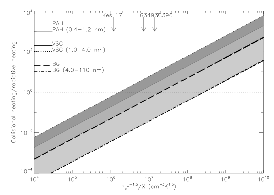
Figure 5: Comparison of the ratio of collisional heating to radiative heating. The abscissa is the quantity $n_{e}T^{\frac{3}{2}}/X$, which, for a given grain size determines whether collisional or radiative heating is dominant. The radiation field employed is for case B radiation and the strength is adopted from the DUSTEM fitting. The 6 lines are the locus for the three dust species, PAHs, VSGs, and BGs and the grey shading is darkest for PAHs and lightest for BGs. Note that the size of the largest PAHs and the smallest VSGs is the same and that the two lines overlap in the plot. Each species has two lines associated with it; the largest and smallest particles in the size distribution. The dashed line indicates equal contribution from radiative and collisional heating. The radiation field for the SNRs is found to be higher than that in the interstellar medium. Representative values for three SNRs are marked.

Figure 5 shows that radiative heating is dominant for BG. The situation is more complicated for the PAHs where in some cases, e.g. 3C396, the contribution from collisional heating may be significant. The PAH or VSG could be heated by collisional heating as well as the radiative heating. If there is a strong contribution from collisional heating, we will overestimate the PAH component in our fits relative to the VSG and BG components. The dominance of collision vs. radiation heating depends on exact local conditions of electron density, temperature and efficiency of energy transfer from the electron to the grain. In our estimates, a number of assumptions are used. One assumption is that electron density is the same as electron density derived from the Fe lines which is observed with the narrow IRS slit while dust is covered by the wider MIPS SED slit. Other uncertainties are local X-ray temperature, density and ionization rate.

Moreover, many of sample SNRs show center-filled X-ray morphology (Combi et al. 2010; Yusef-Zadeh et al. 2003; Harrus & Slane 1999; see references in Hewitt et al. 2009; Rho & Petre 1998) whereas our infrared images show shell-like morphology. Therefore, it is less likely that collisional heating from the X-ray emitting gas is important since the SNR is bordering upon the nearby molecular cloud as we have detected H₂ emission for most sample SNRs. An exception is G11.2-0.3 where both the X-ray and infrared morphology are shell-like. For the case of G11.2-0.3, a strong correlation between X-ray and IR brightness, a poor fit of the dust continuum by the DUSTEM model, the presence of fast shocks indicated by the Ne line ratios and its young age ($\sim$ 2000 yr, inferred from the pulsar), may indicate a picture where multiple physical processes are present. This would complicate the determination of the dominant heating mechanism. More accurate estimation for individual cases should be examined with a combined study of infrared and X-ray data. This is out of the scope of this paper.

4.2 Modifications to the DUSTEM code

We have used a beta version of the DUSTEM model by Compiègne et al. (2008) to fit the dust emission from the SNRs. The model is an update of the dust model by Desert et al. (1990). It has been expanded by Bernard et al. (2008) and Compiègne et al. (2011), where the model is described in more detail. The model and the fitting routines have been modified in several ways for the purpose of this study. Note that some of this modifications are now standard in the publically available version of the code. Instead of only handling a scaling of the local ISRF, now any spectral shape of the radiation field can be used over the wavelength range 0.09–1.6 $\mu$m. We also modified the code to handle the collisional heating only. The electron densities and temperatures determined from the ionic lines are not sufficiently high to be able to reproduce the observed SEDs. We conclude that the model with only the collisional heating is not appropriate for this study. Unfortunately the current code can not simultaneously handle both radiative and collisional heating. We will defer this as future work. We use radiative heating as the dominant heating mechanism in SNRs for further fits and discussion in this paper.

The fitting of the SEDs is done using the method described in Bernard et al. (2008). Each of the dust species and the strength of the radiation field are taken as free parameters in the fit. This gives a total of 4 free parameters in the fit. We are mainly interested in the relative abundances of the different dust species and to compare with the general ISM. We have therefore re–fitted some of the reference SEDs presented in Bernard et al. (2008) and Dwek et al. (1997) using the modified code. The resulting abundances of the LMC and the Milky Way agreed well with those previously published.

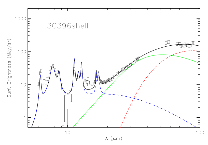
Figure 6: The DUSTEM fit for 3C396shell. The spectrum has been de–reddened based on the foreground hydrogen column density and emission lines have been removed by Gauss fitting. The PAH contribution is shown as the blue line, the VSG contribution as the green line, and the BG contribution is shown as the red line. The total fit is shown as the continuous black line. The values for the best fit parameters are given in Table 5.

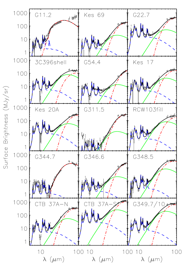
Figure 7: The DUSTEM fit for each SNR adopting a case B type radiation field. The spectra have been de–reddened and atomic and molecular emission lines have been removed by Gauss fitting. The PAH contribution is shown as the blue line, the VSG contribution by the green line, and the BG contribution is shown as the red line. The total fit is shown as the continuous black line.

4.3 Dust Spectral Fitting and Characteristics of Dust Continuum

The DUSTEM model assumes three dust species, PAHs, small carbon grains, or VSGs, and larger silicates, or BGs. The size ranges of the dust species are 0.4–1nm, 1–4nm, and 4–110nm for the PAHs, VSGs, and BGs, respectively. Compared to the original description in Desert et al. (1990), the PAH optical properties were modified to match the ISO spectrum of the diffuse MW ISM (see Compiègne et al., 2008).

We fit the mass abundances of each dust species (Y_PAH, Y_VSG, Y_BG) as well as the strength of the radiation field $F(\lambda)$ (X_F(λ)) for Case B as discussed above. The abundance is the dust mass to gas mass ratio assuming a hydrogen column of $N_{H}=10^{20}cm^{-2}$, which is the expected column density for a molecular gas density of $10^{4}~{}cm^{-3}$ and a shock width of $10^{16}~{}cm$.

For all three dust species, a MRN power-law size distribution is assumed (Mathis et al., 1977). The slopes and size ranges are the same as provided in the updated DUSTEM code as described in Compiègne et al. (2008). The radiation field has been changed from a standard ISRF to the shape predicted from Case B recombination. Thus, each fit has four free parameters: the 3 dust species and the strength of the radiation field. We tried to fit the spectra by changing the slopes of grain size but we concluded that our current data are not sensitive enough to measure the slope. The slope of the long wavelength part of the SED is very sensitive to the radiation field and BG abundances and the spectra between 30-40 $\mu$m is sensitive to VSG abundances. For a given radiation field, the errors of each of the three dust abundances is typically on the order of 20%. Uncertainties in the background subtraction amount are $\sim$10% and are included in the error estimate above.

Figure 6 shows the fit to the shell of 3C396 in detail and Figure 7 shows DUSTEM fits to all the observed SNRs. A reasonable fit was obtained in most of cases with a few notable exceptions such as G11.2-0.3 where the long wavelength part of the fit shows significant departure from the SED data and for G54.4-0.3 where there is a discrepency at 12–20$\mu$m. The fit results are listed in Table. 5 where the fits for the MW and the LMC are also provided (Bernard et al., 2008). The reduced $\chi^{2}$ ranges between 3-12. Systematically higher residuals between the models and spectra are shown between 15 and 20 $\mu$m, resulting in higher reduced $\chi^{2}$. This is likely due to the model being relatively crude in modeling the PAHs.

Our primary conclusions from our spectral fitting are the following. A dust model composed of PAHs, VSGs and BGs provides a reasonable fit to the SEDs of the SNRs. All the SNRs show evidence for PAH emission. Typically the radiation field is 10-100 times larger than the solar neighborhood interstellar radiation field. The strength of the radiation field is consistent with being created from the shock. Two SNRs, G11.2-0.3, and G344.7-0.1 show no to little evidence for VSGs and a lower PAH/BG ratio than observed in the diffuse interstellar medium and the LMC. The lack of VSG emission for these two young SNRs is in agreement with the results for CasA (Rho et al. 2008). However, we note that for G11.2-0.3 the fit is not very good and it is thus not clear if the model is applicable in this case

4.4 Individual Supernovae: Dust fitting and Shock Parameters

We discuss the physical parameters for the SNRs that were not presented in Hewitt et al. (2009). The characteristics of the shocks discussed are based on the ionic lines.

G11.2-0.3 The morphology of the radio emission from the SNR is a clumpy shell which is also seen in the MIPS image with a diameter of 4′. Green (1988) argues the SNR is young and at a distance of $\sim$5 kpc based of the HI data by Becker et al. (1985). Green (1988) favors the short distance due to the youth of the SNR and the large physical size the SNR would have if it was placed at the far distance of $>$26 kpc. A pulsar associated with G11.2-0.3 is found with a period of 65 ms (Torii et al., 1997) and an age of $\lesssim$ 2000 yr (Kaspi et al, 2001). The hydrogen column towards G11.2-0.3 was found by Chandra observations to be 2$\times 10^{22}cm^{-2}$ (Roberts et al., 2003).

For G11.2-0.3, the fit to the MIPS SED is very poor. The reasons for the discrepancy between the model and observations are not entirely clear, especially since the fit to the shorter wavelength observations is relatively good, of similar quality as for most of the other SNRs. It is worth noting that the off position for the MIPS SED was adopted from another set of observations for this SNR. In addition, another plausible possibility is that there is some cold dust along the line of sight that is influencing the long wavelengths. Since the SNR is located only 11 degrees from the Galactic center, the line of sight is rather confused. Future longer wavelength observations will help decipher if the latter is the case. It is evident from the data already at hand, however, that we see the 20 $\mu$m silicate feature in emission for this SNR. There are similar hints for silicate emission in G344.7-0.1. This is to our knowledge the first time silicates are seen in emission in an interacting SNR.

The IRS spectrum shows a rich spectrum of H₂ lines, and ionic lines, particularly iron lines. Utilizing the low excitation lines we find that a J shock into a pre–shock medium of $10^{3-4}$ $cm^{-3}$ and a shock velocity of $\sim 50-80$ $kms^{-1}$ (Hollenbach & McKee, 1989) reproduce the majority of the ionic lines measured. The exception is the [Fe II] line at 24 $\mu$m that is brighter than predicted.

The [Ne III] to [Ne II] ratio is very high, 2.7, suggesting there is in addition a very high velocity shock ($\geq$ 400$kms^{-1}$) propagating into a low–density medium, 100 $cm^{-3}$ or less. The shock model comparison for the [Ne III] to [Ne II] ratio is based on the models of Hartigan et al. (1987) and McKee et al. (1987), and the ratio dependency of the shock velocity is shown in Figure 6a of Rho et al. (2001). We continue to use the same shock models for comparison with the observed line brightnesses below.

G22.7-0.2 Relatively little is known about the partial shell SNR G22.7-0.2. The distance has been estimated with the $\Sigma-D$ relation to be $\sim$3.7 kpc (Case & Bhattacharya, 1998). At the same distance, a molecular cloud has been identified in CO observations. We have used CO data (Dame et al., 2001) to examine the distance and the line of sight column density. Integrating the CO emission up the velocity of the molecular cloud at 3.7 kpc provides a hydrogen column of 7.8$\times 10^{22}~{}cm^{-2}$. However, due to the very large hydrogen column compared with the distance of the SNR and based on the relatively poor fit with DUSTEM using the value of 7.8$\times 10^{22}~{}cm^{-2}$, we have experimented with PAHFIT (Smith et al, 2007) to estimate the extinction. We find that the best fit column density is high, $\sim$9$\times 10^{22}~{}cm^{-2}$. However, we also find that a fit that is almost as good can be obtained with a lower hydrogen column. A hydrogen column as low as 1.5$\times 10^{22}~{}cm^{-2}$ provides a fit that is only 10% worse in a chi square sense than the best fit value. We therefore use the extinction value of 7.8$\times 10^{22}~{}cm^{-2}$ determined directly from the CO measurements.

There is no detection of [Ne III] in G22.7-0.2. The lines of [Ne II], [Fe II] at 26 $\mu$m and [Si II] are detected. Comparison with shock models implies a shock of $\sim$ 90 $kms^{-1}$ propagating into a medium with a density of $10^{3}cm^{-3}$.

G311.5-0.3 G311.5-0.3 is a relatively small (4′ diameter) shell SNR. The distance has been estimated by the $\Sigma-D$ relation to be 12 kpc, whereas emission from CO data has given a radial velocity of $v=+39.7~{}km~{}s^{-1}$ which gives a distance of 14.8 kpc. The detection of H₂ emission implies an interaction with molecular clouds so we have adopted the distance of 14.8 kpc for this study. The total hydrogen column density is 2.5$\times 10^{22}~{}cm^{-2}$ obtained from CO data(Dame et al., 2001). To our knowledge, there has been no detection of OH masers or other indications of interaction with a molecular cloud so our H₂ line detection is likely the first evidence of such an interaction.

The ionic lines suggest a moderately fast shock, 40–90 $kms^{-1}$ propagating into a medium with an initial density of $10^{4}$ $cm^{-3}$. The [Ne III] to [Ne II] ratio points towards either a shock of 100 $kms^{-1}$ with an electron density of $10^{3}$ $cm^{-3}$ or a faster shock, $\sim 170$ $km~{}s^{-1}$ and an electron density of 100 $cm^{-3}$.

RCW 103 RCW 103 is a well studied young ($10^{3}~{}yr$) shell morphology SNR. The distance has been estimated through HI absorption to be 3.3 kpc, based on a velocity of $-56$ km $s^{-1}$ (Caswell et al., 1975). The hydrogen column has been estimated both through X–rays (Gotthelf et al., 1999) and near–infrared spectroscopy (Oliva et al., 1990) and has been found to be 7$\times 10^{21}~{}cm^{-2}$. Previous near–infrared and ISO observations have identified H₂ lines slightly outside the SNR, indicating the material has been heated by soft X–rays (Oliva et al., 1990, 1999).

Due to the size of RCW 103 and the extended emission from the shock, the local off positions for the short low observations are located within the shocked material. There is little dust continuum associated with the parts of the shock that are used as sky background. However, there are emission lines present from the shock which results in an over subtraction of these lines in the on position. We have masked out the regions where the over subtraction have produced negative residuals in the continuum spectrum.

The ionic lines suggest a shock propagating with a velocity of some 80 $kms^{-1}$ into a pre-density of $10^{4}$ $cm^{-3}$. However, the [O I] line is too weak compared to that predicted by Hollenbach & McKee (1989) for a velocity of 80 $km~{}s^{-1}$ and a density of $\sim 10^{4}cm^{-3}$. The model predicts a surface brightness of $\sim 10^{-2.3}ergs^{-1}~{}cm^{-2}~{}sr^{-1}$. Although a small amount of [O I] emission can have been subtracted with the diffuse sky emission, it cannot explain this large difference. The current determination of the [O I] surface brightness flux is in good agreement with the measurements by Oliva et al. (1999). The [Ne III] to [Ne II] line ratio of 0.37 suggest either a shock with a velocity of 100 $km~{}s^{-1}$ and an electron density of 1000 $cm^{-3}$ or a faster shock, 210 $km~{}s^{-1}$ and $n_{e}=100$ $cm^{-3}$.

Kes 20A Little is known about the SNR Kes 20A. Whiteoak & Green (1996) identified a well defined eastern arc of the SNR and a weaker western arc. Based on CO line data, we have estimated a radial velocity of +30 $km~{}s^{-1}$, resulting in a distance of 13.7 kpc. We have found no estimate of the foreground hydrogen column in the literature. Instead we have used CO observations as for G22.7-0.2. By integrating the emission up to the velocity of the SNR, we estimate a total H₂ column of 4.19$\times$ 10²² cm^-2, which corresponds to a hydrogen column of 8.4$\times$10²² cm^-2. The shortest wavelength slit does not extend far enough to completely extend to a spatial region devoid of radio emission. Thus, the whole slit is likely within the shock. However, comparing with the IRAC images, it is evident that there is little emission and the sky position is a good estimate of the background emission. Kes 20A shows a very limited number of ionic lines. Only [SiII] (34.82 $\mu$m) and [Fe II] (35.35 $\mu$m) are detected. Both lines indicate a relatively low velocity shock ($V_{s}\sim 35-70~{}km~{}s^{-1}$) into a low density medium ( $n_{0}\sim 10^{3}~{}cm^{-3}$).

G54.4-0.3 G54.3-0.3 is a large shell–like SNR in a complex region. The distance has been estimated to 3 kpc based on the detection of a molecular cloud and the association of the SNR with OB associations and HII regions (Junkes et al., 1992). The hydrogen column has been estimated from ROSAT X–ray data and is found to be $10^{22}~{}cm^{-2}$(Junkes, 1996). There has been previous identification of a molecular cloud in the vicinity of G54.3-0.3 but direct evidence for interaction of the SNR with surrounding molecular material was not shown.

G54.4-0.3 is another SNR where only few ionic lines are observed. The [Fe II] lines at 26 and 35 $\mu$m suggest a shock into a low density medium ($10^{3}~{}cm^{-3}$), which is confirmed by the detection of [SiII]. The shock velocity determined from the 3 lines is in the range 40–80 $km~{}s^{-1}$.

G344.7-0.1 SNR G344.7-0.1 is an asymmetric shell SNR in the radio. The main features of the shell can be seen in the MIPSGAL image except for the western direction where there is little enhanced emission at 24 $\mu$m. The distance has been estimated from the $\Sigma-D$ relation to be 14 kpc (Dubner et al., 1993). Based on ASCA X–ray observations the hydrogen column was estimated to be 5$\times 10^{22}~{}cm^{-2}$ (Yamauchi et al., 2008). No OH masers have been associated with this SNR (Green et al., 1997).

The [Ne III] to [Ne II] line ratio of 0.54 suggests a high velocity shock of $\sim 280~{}km~{}s^{-1}$ and an electron density of 100 $cm^{-3}$. The ionic lines further suggest that the pre-density material had a density of some $10^{4}~{}cm^{-3}$ and that the shock velocity is some 80 $km~{}s^{-1}$. The models of higher density shocks predict stronger [O I] and [SiII] lines than observed.

CTB 37A CTB 37A is a poorly defined shell SNR overlapping with G348.5-0.0 and CTB 37B. Its distance has been constrained to be between 8 and 11 kpc. We have chosen the distance of 11 kpc that is associated with the HI emission feature. Chandra X–ray observations have determined a hydrogen column of 3.2$\times$10²² cm^-2 (Aharonian et al., 2008). Frail et al. (1996) detected several OH masers associated with the shell of CTB 37A.

The region is very complex and the SNR covers a large area on the sky. The LL2 does not extend completely outside the radio emission of the SNR. However, the IRAC and MIPS 24 $\mu$m images show negligible emission in the outer regions covered by the IRS long slit. We have compared with the IRAC images and the 24 $\mu$m image that there is little to no excess continuum emission in the outer parts and we have used that outer part as our sky position.

For CTB 37A-N, the fit is mediocre at the 9.5 $\mu$m range. This is in contrast to CTB 37A-S where the short wavelength range is fit relatively well. A likely explanation is uncertainties in the dereddening of the source. For CTB37A, one reddening value is adopted for the whole SNR, despite the fact that it covers 15′radius area close to the Galactic center. It is thus likely the reddening can vary across the SNR due to unrelated foreground material. Since the silicate absorption feature is a strong function of the extinction compared to the rest of the mid–IR extinction curve, the fit can be substantially improved by increasing the extinction. However, in order to provide a much better fit, the hydrogen column has to be almost doubled compared to the value determined from X–rays. Even altering the hydrogen column to $5.5\times 10^{22}~{}cm^{-2}$ only changes the reduced $\chi^{2}$ by $\sim 20\%$. The ratio of dust species remain almost the same. The quality of the fit improves a bit, the reduced $\chi^{2}$ is 3.5 compared to 5 adopting the X–ray determined hydrogen column. The subsequent analysis is based on the best fit adopting the hydrogen column determined from the X–ray. The conclusions do not change significantly adopting the higher hydrogen column.

We find the shock characteristics to be slightly different at the two locations observed within CTB 37A. For the CTB 37A-N position we find a density of $10^{3.5}~{}cm^{-3}$ and a shock velocity of $\sim 100~{}km~{}s^{-1}$ whereas the CTB 37A-S region appears a bit denser, $10^{4}~{}cm^{-3}$ and the shock is slower, $\sim 75km~{}s^{-1}$. The observed [O I] line is too weak for such dense shocks where a surface brightness of $\sim 10^{-2}erg~{}s^{-1}~{}cm^{-2}~{}sr^{-1}$ is predicted.

5 Discussion

We present the results for the DUSTEM fitting to the SEDs of the SNRs. The ratio of the dust species is determined and is compared with the same ratios for Galactic plane dust and dust in the LMC interstellar medium. We further discuss the results in view of dust destruction models.

5.1 Dust Properties of SNRs

We present the fitting results using Case B radiation field in Table  5 and the results are further summarized in Figure 8. The radiation field in SNRs is higher than those of ISM and the average value of the Milky way and LMC; this conclusion is independent of the spectral shape of the radiation field. Most of the SNRs are well fit with a radiation field of 50–200 times the local interstellar radiation field, in general agreement with the modified black body fits performed above. Although the ISRF is expected to be stronger in the inner parts of the Galaxy where most of the known SNRs reside, we do not expect this to be able to account for the high radiation field. Typically, closer to the Galactic center, the ISRF is only a few times the strength of the local ISRF. Instead, we suggest below that the enhanced radiation can be explained by hydrogen recombination. Note that since the absolute gas column density of the SNR shock front is not known, we cannot compare the absolute abundances between SNRs or the Milky Way. However, the ratios can directly be compared between different SNRs and other environments, e.g. the interstellar medium.

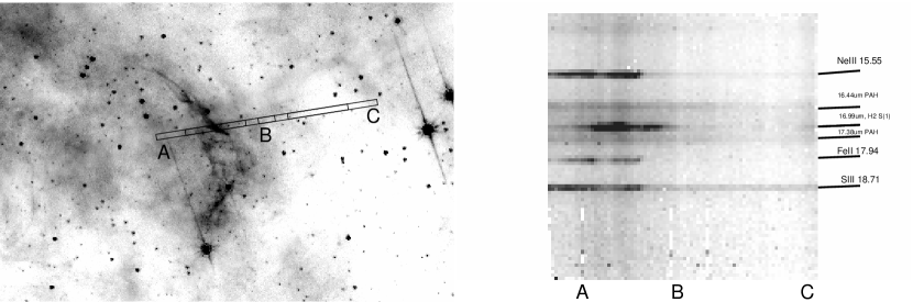
Figure 9: Left: a Spitzer GLIMPSE 8 $\mu$m image of Kes 17. Overlaid is the four slit positions of the LL2 module. Right: The combined 2 dimensional spectrum from the four LL2 sub slits. Enhanced PAH emission from 15–20$\mu$m is seen at the position of SNR shell (A to B on slit) indicating that PAH emission is associated with the SNR Kes 17.

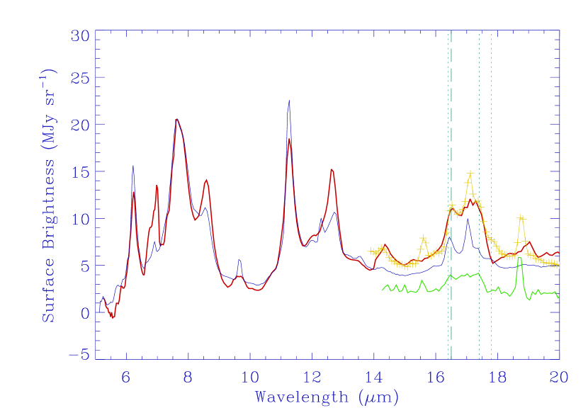
Figure 10: Comparison of PAH emission in the SNR Kes 17 (red curve) with those of LkH$\alpha$ 234 (PDR: blue) and NGC7331 (yellow). The 15-20 $\mu$m PAH emission in the background of Kes 17 (green) is also compared, showing that the plateau bump is weaker than that of Kes 17 and that the shape was somewhat altered. The shape of the PAH emission between 5-14 $\mu$m in Kes 17 is almost identical to that in the Galactic background, suggesting little processing of the smallest grains.

The dust spectral fitting indicates the presence of PAH emission in most of SNRs as shown in Figure 10. The dip centered at 9.7 $\mu$m could indicate either presence of PAH emission or high extinction from silicates. However, the feature is present after the foreground extinction correction of the SNRs and is thus likely due to PAH emission. We here show a detailed example of PAH emission using an example of the SNR Kes 17. Figure 9 shows the location of the slits covering Kes 17. The ”A” location is within the SNR, and the location between the B and C is the surrounding ISM. The PAH emission around 17 $\mu$m is enhanced at the shell of the SNR Kes 17. The PAH spectrum of Kes 17 is shown in Figure 10 where it is compared with the emission from LkH_α 234 and NGC7331, a PDR and a nearby spiral galaxy with strong PAH emission, respectively. The PAH emission is always detected in our background spectra since all the SNRs are located in the Galactic plane. However, the PAH emission is clearly enhanced in the shocked region and is present after background subtraction. The 15-20 $\mu$m PAH bump in Kes 17 is stronger than that of LkH$\alpha$ 234 whereas the PAH features between 5-14 $\mu$m are almost identical (the slight differences are likely due to residuals from line subtraction or extinction correction). However, the 15-20 $\mu$m feature of Kes 17 is flatter than that of the PDR and the feature shows a plateau shape. The feature is similar to that of NGC 7331. The ratio of the emission from the 15-20 $\mu$m plateau to the 6.2 $\mu$m PAH feature is 0.4 for Kes 17 and other H₂ emitting SNRs, similar to NGC 7331 but larger than for the PDR. This ratio is significantly smaller than that of the young SNR N132D (Tappe et al., 2006). The difference between our sample and N132D is the environments of SNRs. Many of the interacting SNRs are in a dense molecular cloud environment with a slow shock, while N132D in less dense environment has a strong shock which significantly destroy small PAHs. We note that whenever we detected PAH emission in SNRs there is PAH emission in the background as well (see Figure 9), indicating the PAH emission is from shock processed dust instead of shock generated dust. For some of the observed SNRs, one or more of the slits did not cover a background region. Full spectral mapping would be needed for further detailed studies of PAH processing through shocks.

The three different dust components dominate in different parts of the observed SEDs. Shortwards of 20 $\mu$m the PAH component dominates the spectrum. Between 20 $\mu$m and up to 30 $\mu$m the emission from VSGs is in general the main contribution, whereas the MIPS SED traces the BGs. Between 30–35 $\mu$m the VSGs and BGs can both contribute depending on the strength of the radiation field. For two of the SNRs, G11.2-0.3 and G344.7-0.1, the SEDs can be fit without the need of VSGs. We discuss these two SNRs separately.

The shape of the continuum is well reproduced by the model for each of the sample SNRs except G11.2-0.3 and G344.7-0.1. Where the model in general fails to fit the data in detail is in the shape of the PAH features at shorter wavelengths. The PAH feature at 12.3 $\mu$m is not well reproduced. It appears the observations have a red ’wing’ that is stronger than predicted. This is likely not an anomaly with the PAH emission from the shock heated dust. In similar spectral fitting to the Horsehead Nebula, Compiègne et al. (2008) also finds that the model underpredicts the emission slightly in this wavelength range.

The reduced $\chi^{2}$ for the fits are in general moderately poor. A closer look at the individual fits shows that a large part of the discrepancy is due to differences in the PAH dominated part of the SEDs. Here we note the origin of the discrepancy between the model and the observed PAHs but defer a detailed discussion of the PAH evolution to a future paper. We further note that the reduced $\chi^{2}$ determined for the SNRs is similar to the reduced $\chi^{2}$ for the Galactic plane measurements. We thus conclude the model fits to the dust from the SNRs captures the fundamental large scale features of the dust emission.

The abundance of each of the three dust species for each SNR is given in Table 5. The SNRs can be placed into two categories. The majority of the SNRs have ratios of VSGs to BGs and PAHs to BGs that are higher than those observed in the diffuse interstellar medium of Galactic plane. This group includes G22.7-0.2, Kes17, 3C396, CTB37A-S, RCW103, kes 20A, and G349.7+0.2. The radiation field derived for this sample is intermediate in strength, much lower than that of the group with a small ratio of carbon to silicate grains. A smaller group has a low ratio of carbon grains to silicates, including G11.2-0.3 and G344.7-0.1. This group is also further characterised by a very high radiation field, sufficiently high to see silicates in emission at 20 $\mu$m.

The derived PAH abundances are also in general higher than observed in the MW plane. The larger error bars for the PAH abundances, due to their general low abundance relative to the VSGs and BGs, makes it difficult to find any correlation between the derived PAH abundances and other parameters. However, their overabundance relative to the MW plane support a shattering scenario for dust processing together with the results for the VSGs. Note that the two SNRs with low VSG to BG ratios also have a low abundance of PAHs which confirms the shattering scenario.

5.2 Dust Processing Through Sputtering And Shattering

The ratios of carbon dust (PAHs and small grains) to silicates can be explained through dust destruction scenarios. Two dust destruction scenarios are sputtering (e.g. Dwek et al., 1996) and shattering (e.g. Borkowski & Dwek, 1995; Jones et al., 1994) which are discussed below.

5.2.1 Sputtering

It is predicted that sputtering will alter the grain size distribution in fast shocks (Dwek et al., 1996). The efficiency of sputtering depends on size of grains and is most efficient on smaller grains resulting in a mass distribution with a relative deficit of small grains compared to the general ISM grain size distribution.

We find for a low value of both the PAH and VSG abundance relative to the BG abundance for G11.2-0.3, G344.7-0.1, and G311.5-0.3. In fact, the SED for G344.7-0.1 suggest the presence of no VSGs at all and only a small amount of PAHs. The situation is less clear for G311.5-0.3 since the emission at all wavelengths is rather weak and the abundances measured, for all three dust species, is uncertain, due to a complicated background diffuse Galactic background near G311.5-0.3. For G11.2-0.3 and G344.7-0.1, the neon line measurements suggest a fast shock (280 $kms^{-1}$) into a medium with an initial density of some 100 $cm^{-3}$. Comparing with the calculations by Dwek et al. (1996) we see that at these temperatures and densities, significant amount of sputtering can occur, which thus provides a likely explanation for the low abundance of PAHs and VSGs relative to BGs in G11.2-0.3 and G344.7-0.1. Note also that for G11.2-0.3, and G344.7-0.1 we see evidence for the silicates in emission at 21 $\mu$m. We find sputtering is efficient at high shock velocities and relatively low densities as observed in G11.2-0.3, and G344.7-0.1 compared to those observed in the other interacting SNRs where the sputtering in general do not play a dominant role as suggested by (e.g. Jones et al., 1994). A more sophisticated dust model combined with an abundance analysis may be required to understand the role of sputtering in the two young SNRs.

5.2.2 Shattering

The ratio of Y(VSG)/Y(BG) ranges between 0.11-1.4 for the SNRs not showing silicates at 21 $\mu$m in emission . The ratio in SNRs is a factor of a few larger than those of the MW (0.13) and the LMC for most of the SNRs. We interpret the higher ratio is indication of shattering, big grains being destroyed by shocks turning them into small grains. Jones et al. (1994) suggest that in dense, relatively slow shocks, grain processing through shattering will occur. Contrary to the case of sputtering, large grains are predominately affected and silicates are more vulnerable than graphite grains (Jones et al., 1994). For the typical shock velocities determined for the shocks, shattering is expected to be efficient for grains larger than some 400–1000Å which will be shattered and we thus expect shattering to occur for the BGs.

It is possible that some of the BGs are shattered into the size distribution of the VSGs. The ratios of VSG to BG seem to be higher for the high speed shocks. However, the standard VSGs are predominantly comprised of carbon and silicates. Silicates are characterized by strong emission features at 10 $\mu$m and 20 $\mu$m. However, these features are not observed in most of the SNR spectra. We have thus examined whether silicate grains with a size range and distribution similar to that of the VSGs would produce emission features inconsistent with the observed spectra. The strength of the silicate emission features depend on the strength of the radiation field. A Case B radiation field 500 times stronger than the default strength, the strength of the 10 $\mu$m emission feature is very weak compared to the emission from a similar amount of carbon VSGs (in mass) irradiated by the same radiation field. At 20 $\mu$m the emission peak is comparable in strength to the emission from the carbon VSGs. Significantly higher radiation fields are required to produce a substantial 10 $\mu$m feature compared to the strength of the PAHs. However, the only two SNRs where such a strong radiation field is observed are already fit purely by PAHs and BG silicates and no VSGs. It is therefore possible to have a population of silicates towards small sized dust particles and not have them show up as emission features at shorter wavelengths.

Since the BGs are over five times as abundant than the VSGs in the ISM (in mass), even a small processing of BGs into VSGs would increase the ratio of the two substantially. For example, a shattering of 10% of the BGs into VSGs will increase an initial VSG to BG ratio of 0.2 to 0.3. If 50% of the BGs are processed to VSGs the ratio will be 1.2, assuming all the shattered fragments end up as VSGs. Jones et al. (1994) calculates the grain size where 50% of the grains will be reprocessed for a given shock velocity. For shocks faster than $\sim$ 100 km/s, the limiting grain size is $\sim$400 Å. Almost all grains larger than the critical size will be destroyed and almost all grains smaller will survive. We can thus calculate the predicted amount of large grains shattered from the input MRN distribution. Adopting the minimum and maximum grain size from the DUSTEM code and a critical size of 400Å, we find that 46% of the large grains will be destroyed by a shock faster than 100 km/s. Thus, the ratio of carbon grains (which are too small to be affected by shattering) to the large silicates would double by the removal of the large grains alone with a further increase from the smaller particles produced in the shattering process. A shock speed of 100 $kms^{-1}$ is where the smallest grains are affected. At both lower and higher speeds only larger grains will be completely shattered.

The majority of the shock velocities determined above are in the range 50–80 $kms^{-1}$ and we would thus expect less of the BGs being shattered than for a 100 $kms^{-1}$ shock, which is indeed what is observed for most of the SNRs. In principle we should see a monotonic dependence of the VSG to BG ratio as a function of shock speed in that, the slower the shock, the less shattering occurs. There is no strong correlation seen which is likely to be due to the uncertainty in the derived shock velocities (see above). However, there is a tendency for the highest VSG to BG ratios to correspond to the highest derived shock velocities. Further, as shown for a few of the SNRs (e.g. G11.2-0.3, Lee et al. (2009), and 3C396, Koo et al. (2007)) the H₂ emission seems to be more localized whereas the [Fe II] emission is a bit more diffuse. All SNRs where the shock speed has been determined to be larger than $60kms^{-1}$ have an increased VSG to BG ratio and those with slower shocks tend to have ratios located closer to the ratio found in the MW plane. The two exceptions are Kes 20A and RCW 103. Due to the limited number of ionic lines for Kes 20A, the shock velocity is somewhat uncertain.

Table 5: The parameters obtained for the DUSTEM fits adopting a Case B radiation field. The dust abundances are relative mass fractions to a fiducial hydrogen column density of N${}_{\mathrm{H}}=10^{20}cm^{-2}$. X is the strength of radiation field relative to the case B radiation field of which the total energy is normalized by the ISRF. $\chi^{2}$ is the reduced goodness of the fit using DUSTEM model.

Object	Y(PAH)	Y(VSG)	Y(BG)	Y(TOT)	X	Reduced $\chi^{2}$	$\frac{Y(PAH)}{Y(BG)}$	$\frac{Y(VSG)}{Y(BG)}$
MW (plane)	3.11E-4	1.09E-3	8.42E-3	9.82E-3	1.46	7.87	3.69E-2	1.3E-1
MW (diff)	4.83E-4	6.38E-4	4.68E-3	5.8E-3	0.8	11.87	10.3E-2	1.36E-1
LMC	9.7E-5	3.47E-4	3.16E-3	3.6E-3	1.85	1.12	3.07E-2	1.1E-2
G11.2	1.8(0.1)E-5	0.0(0.0)E 0	1.0(0.1)E-3	1.0(0.1)E-3	4.8(0.2)E+3	12	1.8(0.1 )E-2	0.0(0.0 )E 0
Kes 69	2.4(0.4)E-3	7.9(1.5)E-3	3.3(0.5)E-2	4.4(0.5)E-2	3.6(0.6)E+1	7	7.3(1.5 )E-2	2.4(0.6 )E-1
G22.7	1.8(0.3)E-2	2.0(0.5)E-2	7.4(1.3)E-2	1.1(0.1)E-1	3.7(0.7)E+1	9	2.5(0.6 )E-1	2.7(0.8 )E-1
3C396cent	1.3(0.2)E-2	2.1(0.4)E-2	7.2(1.2)E-2	1.1(0.1)E-1	3.8(0.6)E+1	9	1.8(0.4 )E-1	2.9(0.7 )E-1
3C396shell	3.9(1.2)E-3	1.7(0.6)E-2	1.2(0.3)E-2	3.3(0.7)E-2	6.6(2.1)E+1	6	3.2(1.3 )E-1	1.4(0.6 )E 0
G54.4	9.9(1.9)E-3	2.0(0.4)E-2	9.3(2.2)E-2	1.2(0.2)E-1	9.9(2.0)E+0	12	1.1(0.3 )E-1	2.2(0.7 )E-1
Kes 17	4.4(0.9)E-3	1.2(0.3)E-2	2.3(0.5)E-2	4.0(0.6)E-2	4.9(1.0)E+1	3	1.9(0.5 )E-1	5.2(1.7 )E-1
Kes 20A	1.5(0.3)E-2	2.7(0.7)E-2	5.5(1.3)E-2	9.7(1.5)E-2	3.2(0.7)E+1	5	2.8(0.9 )E-1	4.9(1.7 )E-1
G311.5	3.6(0.4)E-4	4.7(0.6)E-3	4.4(0.4)E-2	4.9(0.4)E-2	4.5(0.4)E+1	7	8.1(1.1 )E-3	1.1(0.2 )E-1
RCW103fill	5.6(1.6)E-3	3.4(1.1)E-2	3.4(1.0)E-2	7.3(1.4)E-2	3.5(1.0)E+1	8	1.7(0.7 )E-1	1.0(0.4 )E 0
G344.7	1.2(0.1)E-4	5.7(0.0)E-9	5.7(0.2)E-3	5.8(0.2)E-3	4.1(0.1)E+2	6	2.2(0.1 )E-2	1.0(0.0 )E-6
G346.6	4.5(0.8)E-3	1.7(0.4)E-2	7.7(1.6)E-2	9.8(1.7)E-2	1.8(0.3)E+1	8	5.8(1.6 )E-2	2.2(0.7 )E-1
G348.5	1.3(0.2)E-3	1.3(0.2)E-2	2.8(0.3)E-2	4.2(0.4)E-2	9.3(1.2)E+1	5	4.8(0.8 )E-2	4.6(0.9 )E-1
CTB 37A-N	3.1(0.4)E-3	9.9(1.8)E-3	3.2(0.4)E-2	4.5(0.4)E-2	7.8(1.0)E+1	6	9.6(1.6 )E-2	3.1(0.7 )E-1
CTB 37A-S	3.0(0.6)E-2	8.2(1.9)E-2	1.7(0.3)E-1	2.8(0.4)E-1	4.5(0.9)E+1	5	1.8(0.5 )E-1	4.8(1.4 )E-1
G349.7	5.6(0.9)E-2	5.0(1.0)E-1	8.2(1.3)E-1	1.4(0.2)E 0	5.6(0.9)E+1	6	6.8(1.6 )E-2	6.1(1.5 )E-1

Figure 8: From top to bottom: The ratio of VSGs, PAHs, and PAH+VSGs to BGs, assuming a Case B radiation field. The ratios determined for the plane of the Milky Way are shown as the solid line in each plot. Most of the dust ratios are above the ratio determined in the MW plane at least at a 2$\sigma$ level. However, a small group of SNRs have ratios of carbon dust to silicates smaller than the MW plane ratio. These are associated with a strong radiation field.

5.3 Integrated Dust Mass

With an estimate of the dust mass within the IRS and MIPS SED beam we can derive the total dust mass in each SNR by assuming the 24 $\mu$m and 70 $\mu$m emission trace the total dust mass. We have integrated the total emission from the SNRs from both the MIPS 24 $\mu$m and 70 $\mu$m images. Even though the derived 70$\mu$m fluxes are in the nonlinear regime we can still estimate the total flux from the SNR. This approach works best for relatively small, well defined SNRs. Examples are G11.2-0.3, G311.5-0.3, G344.7-0.1, and Kes 17 where we can easily trace the emission and where the region is not confused by e.g. HII regions and other bright unrelated objects. We note that for many of the SNRs the total dust mass is a lower limit for the following reason. For the extended SNRs we have used the radio contours in conjunction with a with a visual inspection of the images to identify the regions with dust emission associated with the SNR. We have thus excluded regions in the SNRs close to very bright stars or to regions that appears to be HII regions along the line of sight to the SNR, as is for example the case of CTB 37 near the south position. We therefore will be missing some of the faint dust emission from the SNRs, especially for the large area SNRs as CTB 37, and 3C396. In addition, the central position in 3C396 is located near a very bright star and is not used for the estimate of the total dust mass within the SNR.

Moderately bright stars within the SNR in both the 24 $\mu$m and 70 $\mu$m images have been masked before the flux has been integrated across the SNR. The background level has been estimated from adjacent regions of clear sky and has been subtracted from the emission form the SNR. It is evident from the IRS spectra and the MIPS SED that the broad band emission is contaminated by line emission. In particular the iron line at 26 $\mu$m and the [O I] line at 63 $\mu$m are strong. However, since we have assumed similar properties for the gas and dust within the MIPS SED and IRS beam as for the whole SNR, this fractional contribution will be the same in both cases. Table 6 shows the correction factor (one over the fraction of the SNR emission covered by the MIPS SED ) at 24 and 70 $\mu$m, and the total mass for each the the dust species as well as the total shocked dust mass for the SNR. The total mass was derived using the average of the two correction factors.

Table 6: Integrated dust masses for the SNRs. The total flux associated with each SNR in the 24 and 70 $\mu$m images have been calculated and the dust mass determined from the SED fitting has been scaled accordingly.

SNR	Cor factor (24 $\mu$m)	Cor factor (70 $\mu$m)	PAH mass	VSG mass	BG mass	Total mass
			M⊙	M⊙	M⊙	M⊙
G11.2	2.3e+01	3.8e+01	1.6e-04	0.0e+00	8.6e-03	8.8e-03
Kes69	9.9e+01	1.0e+02	7.3e-02	2.4e-01	1.0e+00	1.3e+00
G22.7	1.4e+02	1.6e+02	4.1e-01	4.5e-01	1.7e+00	2.5e+00
3C396	3.0e+01	8.8e+01	3.6e-01	5.8e-01	2.0e+00	3.0e+00
G54.4	2.3e+01	4.0e+01	3.1e-02	6.4e-02	3.0e-01	3.9e-01
Kes 17	2.7e+01	3.5e+01	1.4e-01	4.0e-01	7.6e-01	1.3e+00
G311.5	2.3e+01	1.1e+01	1.5e-02	1.9e-01	1.8e+00	2.0e+00
RCW 103	1.1e+02	1.3e+02	8.4e-02	5.1e-01	5.0e-01	1.1e+00
G344.7	4.6e+01	0.0e+00	1.2e-02	5.7e-07	5.7e-01	5.8e-01
G348.5	3.7e+00	1.1e+01	2.1e-02	2.0e-01	4.3e-01	6.4e-01
CTB 37	2.3e+02	2.8e+02	1.1e+00	3.4e+00	1.1e+01	1.5e+01
G349.7	6.8e+00	2.1e+00	1.3e+00	1.2e+01	2.0e+01	3.3e+01

The correction factors are very large for many of the SNRs. Often time only a few percent or less of the total dust emission was probed by the MIPS SED. The derived dust masses are therefore only to be considered estimates. Further, it is clear from the derived correction factors between the 24 and 70 $\mu$m images that some uncertainty is inherited here as well. There are several potential reasons for the different correction factors. The most likely is non-linearity effects in the 70 $\mu$m data that will tend to underestimate the flux, in particular from brighter emission spots. We estimate the masses determined to be good within a factor of two to three. Nevertheless, the calculated dust masses are useful to estimate the amount of dust in molecular clouds that is being processed by SNRs. Each SNR appears to be able to heat, and thus shatter, one to several solar masses of dust at any time. Due to the speed of the shock front, it is likely it will penetrate further into the surrounding molecular cloud and further process the dust. Thus, the total amount of dust that can be heated and processed by a single SNR can be up to ten solar masses.

One of the few previous estimates of ISM dust being processed by a SNR was by Reach & Rho (2000). They estimated the dust mass within one ISO LWS beam (80″ FWHM) in 3C391 to be 1 M_⊙. Integrating for the whole SNR would increase this estimate substantially, possible up to 10 M_⊙. However, the two other SNRs analyzed in the same paper, W28, and W44, had an order of magnitude less dust within the beam. Further two of the SNRs had previous dust mass estimates based on IRAS photometry (Saken et al., 1992). They found a total amount of warm dust of 5.6$\times 10^{-3}$ M_⊙ for Kes 17, and 0.17 M_⊙ for G349.7+0.2. Whereas the latter is in good agreement with the mass estimated here, we derive a substantially larger mass for Kes 17. The lower mass derived by Saken et al. (1992) may be due to beam dilution and the limited sensitivity that would leave most of the emission undetected with IRAS. Reach & Rho (2000) estimated the mass within one beam of the ISO LWS camera to be roughly 1 M_⊙, comparable to a typical dust mass found here of 2-3 M_⊙.

We can estimate the time scale for processing an amount of dust comparable to the content in the Galaxy. A rough volume of the Galaxy can be estimated by assuming it is a cylinder with a height of 100 pc and a radius of 15 kpc. A typical SNR expands to some 20 pc and the rate of type II SNRs is roughly $1.9/100~{}yr$ (Diehl et al., 2006). Thus, the time scale is then $\pi\times(15000)^{2}\times 100/(4~{}\pi/3\times 20^{3}/(1.9/100)~{}yr\sim 110~{}Myr$ for Galactic dust to, on average, have been processed once by a SNR shock.

6 Conclusions

We have presented the results from MIPS SED and IRS low resolution spectroscopy of 14 Galactic SNRs. Our main results are the following; 1) We find that they show sign for interactions with a surrounding molecular cloud. This is established through the presence of $H_{2}$ lines and the detection of [O I] at 63 $\mu$m. This almost doubles the sample of known interacting SNRs. 2) The dust continuum varies markedly from SNR to SNR, with relatively large variations in the relative dust species abundances. 3) We find evidence for dust processing by comparing the dust species ratios. 4) The integrated dust mass is estimated for a sub–set of the SNRs. We find typically around 1 M_⊙ of dust is shocked by a SNR interacting with a molecular cloud. 5) We find that the main cooling is occurring through the dust with relatively minor contribution from $H_{2}$ and [O I].

References

- Aharonian et al. (2008) Aharonian, F., et al. 2008, A&A, 490, 685
- Appleton et al. (2004) Appleton, P. N., et al. 2004, ApJS, 154, 147
- Becker et al. (1985) Becker, R. H., Markert, T., & Donahue, M. 1985, ApJ, 296, 461
- Bernard et al. (2008) Bernard, J.-P., et al. 2008, AJ, 136, 919
- Borkowski & Dwek (1995) Borkowski, K. J., & Dwek, E. 1995, ApJ, 454, 254
- Burton et al. (1990) Burton, M. G., Hollenbach, D. J., Haas, M. R., & Erickson, E. F. 1990, ApJ, 355, 197
- Carey et al. (2009) Carey, S. J., et al. 2009, PASP, 121, 76
- Case & Bhattacharya (1998) Case, G. L., & Bhattacharya, D. 1998, ApJ, 504, 761
- Caswell et al. (1975) Caswell, J. L., Murray, J. D., Roger, R. S., Cole, D. J., & Cooke, D. J. 1975, A&A, 45, 239
- Combi et al. (2010) Combi., J. A. et al. 2010, A&A, 523, 76
- Churchwell et al. (2009) Churchwell, E., et al. 2009, PASP, 121, 213
- Compiègne et al. (2008) Compiègne, M., Abergel, A., Verstraete, L., & Habart, E. 2008, A&A, 491, 797
- Compiègne et al. (2011) Compiègne, M., et al. 2011, A&A, 525, A103
- Dame et al. (2001) Dame, T. M., Hartmann, D., & Thaddeus, P. 2001, ApJ, 547, 792
- Desert et al. (1990) Désert, F.-X., Boulanger, F., & Puget, J. L. 1990, A&A, 237, 215
- Diehl et al. (2006) Diehl, R., et al. 2006, Nature, 439, 45
- Draine et al. (1983) Draine, B. T., Roberge, W. G., & Dalgarno, A. 1983, ApJ, 264, 485
- Draine (2003) Draine, B. T. 2003, ARA&A, 41, 241
- Dubner et al. (1993) Dubner, G. M., Moffett, D. A., Goss, W. M., & Winkler, P. F. 1993, AJ, 105, 2251
- Dwek et al. (1987) Dwek, E., Hauser, M. G., Dinerstein, H. L., Gillett, F. C., & Rice, W. L. 1987, ApJ, 315, 571
- Dwek & Arendt (1992) Dwek, E., & Arendt, R. G. 1992, ARA&A, 30, 11
- Dwek et al. (1997) Dwek, E., et al. 1997, ApJ, 475, 565
- Dwek et al. (1996) Dwek, E., Foster, S. M., & Vancura, O. 1996, ApJ, 457, 244
- Frail et al. (1996) Frail, D. A., Goss, W. M., Reynoso, E. M., Giacani, E. B., Green, A. J., & Otrupcek, R. 1996, AJ, 111, 1651
- Gotthelf et al. (1999) Gotthelf, E. V., Petre, R., & Vasisht, G. 1999, ApJ, 514, L107
- Green (1988) Green, D. A. 1988, Ap&SS, 148, 3
- Green et al. (1997) Green, A. J., Frail, D. A., Goss, W. M., & Otrupcek, R. 1997, AJ, 114, 2058
- Green et al. (1988) Green, D. A., Gull, S. F., Tan, S. M., & Simon, A. J. B. 1988, MNRAS, 231, 735
- Guillet et al. (2007) Guillet, V., Pineau Des Forêts, G., & Jones, A. P. 2007, A&A, 476, 263
- Guillet et al. (2009) Guillet, V., Jones, A. P., & Pineau Des Forêts, G. 2009, A&A, 497, 145
- Hartigan et al. (1987) Hartigan, P., Raymond, J., & Hartmann, L. 1987, ApJ, 316, 323
- Harrus & Slane (1999) Harrus, I. M. & Slane, P. O. 1999, ApJ, 516, 811
- Hewitt et al. (2009) Hewitt, J. W., Rho, J., Andersen, M., & Reach, W. T. 2009, arXiv:0901.1622
- Hollenbach & McKee (1979) Hollenbach, D., & McKee, C. F. 1979, ApJS, 41, 555
- Hollenbach & McKee (1989) Hollenbach, D., & McKee, C. F. 1989, ApJ, 342, 306
- Jones et al. (1994) Jones, A. P., Tielens, A. G. G. M., Hollenbach, D. J., & McKee, C. F. 1994, ApJ, 433, 797
- Junkes et al. (1992) Junkes, N., Fuerst, E., & Reich, W. 1992, A&A, 261, 289
- Junkes (1996) Junkes, N. 1996, Unsolved Problems of the Milky Way, 169, 627
- Kaspi et al (2001) Kaspi et al, 2001, ApJ, 560, 371
- Koo et al. (2007) Koo, B.-C., Moon, D.-S., Lee, H.-G., Lee, J.-J., & Matthews, K. 2007, ApJ, 657, 308
- Lee et al. (2009) Lee, H.-G., Moon, D.-S., Koo, B.-C., Lee, J.-J., & Matthews, K. 2009, ApJ, 691, 1042
- Li & Draine (2001) Li, A., & Draine, B. T. 2001, ApJ, 554, 778
- Lu et al. (2008) Lu, N., et al. 2008, PASP, 120, 328
- Mathis et al. (1977) Mathis, J. S., Rumpl, W., & Nordsieck, K. H. 1977, ApJ, 217, 425
- Mathis et al. (1983) Mathis, J. S., Mezger, P. G., & Panagia, N. 1983, A&A, 128, 212
- McKee et al. (1987) McKee, C. F. 1987, Spectroscopy of Astrophysical Plasmas, ed. A. Dalgarno & D. Layzer (Cambridge: Cambridge University Press)
- Ogle et al. (2007) Ogle, P., Antonucci, R., Appleton, P. N., & Whysong, D. 2007, ApJ, 668, 699
- Olbert et al. (2003) Olbert, C. M., Keohane, J. W., Arnaud, K. A., Dyer, K. K., Reynolds, S. P., & Safi-Harb, S. 2003, ApJ, 592, L45
- Oliva et al. (1990) Oliva, E., Moorwood, A. F. M., & Danziger, I. J. 1990, A&A, 240, 453
- Oliva et al. (1999) Oliva, E., Moorwood, A. F. M., Drapatz, S., Lutz, D., & Sturm, E. 1999, A&A, 343, 943
- Osterbrock & Ferland (2006) Osterbrock, D. E., & Ferland, G. J. 2006, Astrophysics of gaseous nebulae and active galactic nuclei, 2nd. ed. by D.E. Osterbrock and G.J. Ferland. Sausalito, CA: University Science Books, 2006,
- Patnaik et al. (1990) Patnaik, A. R., Hunt, G. C., Salter, C. J., Shaver, P. A., & Velusamy, T. 1990, A&A, 232, 467
- Reach et al. (1995) Reach, W. T., et al. 1995, ApJ, 451, 188
- Reach et al. (2006) Reach, W. T., et al. 2006, AJ, 131, 1479
- Reach & Rho (1996) Reach, W. T., & Rho, J. 1996, A&A, 315, L277
- Reach & Rho (2000) Reach, W. T., & Rho, J. 2000, ApJ, 544, 843
- Rho & Petre (1998) ho, J, & Petre, R., 1998, ApJ, 503, 167
- Rho et al. (2001) Rho, J., Jarrett, T. H., Cutri, R. M., & Reach, W. T. 2001, ApJ, 547, 885
- Rho et al. (2008) Rho, J., et al. 2008, ApJ, 673, 271
- Roberts et al. (2003) Roberts, M. S. E., Tam, C. R., Kaspi, V. M., Lyutikov, M., Vasisht, G., Pivovaroff, M., Gotthelf, E. V., & Kawai, N. 2003, ApJ, 588, 992
- Saken et al. (1992) Saken, J. M., Shull, J. M., Garmany, C. D., Nichols-Bohlin, J., & Fesen, R. A. 1992, ApJ, 397, 537
- Shull & McKee (1979) Shull, J. M., & McKee, C. F. 1979, ApJ, 227, 131
- Smith et al. (2007) Smith, J. D. T., et al. 2007, PASP, 119, 1133
- Smith et al (2007) Smith, J. D. T. et al. 2007, ApJ, 656, 770
- Soifer et al. (2008) Soifer, B. T., Helou, G., & Werner, M. 2008, ARA&A, 46, 201
- Tappe et al. (2006) Tappe, A., Rho, J., & Reach, W. T. 2006, ApJ, 653, 267
- Torii et al. (1997) Torii, K., Tsunemi, H., Dotani, T., & Mitsuda, K. 1997, ApJ, 489, L145
- Whiteoak & Green (1996) Whiteoak, J. B. Z., & Green, A. J. 1996, A&AS, 118, 329
- Yamauchi et al. (2008) Yamauchi, S., Ueno, M., Koyama, K., & Bamba, A. 2008, PASJ, 60, 1143
- Yusef-Zadeh et al. (2003) Yusef-Zadeh, F., Wardle, M., Rho, J., & Sakano, M. 2003, ApJ, 585, 319