Scaling of Seismic Memory with Earthquake Size

Abstract

It has been observed that the earthquake events possess short-term memory, i.e. that events occurring in a particular location are dependent on the short history of that location. We conduct an analysis to see whether real-time earthquake data also possess long-term memory and, if so, whether such autocorrelations depend on the size of earthquakes within close spatiotemporal proximity. We analyze the seismic waveform database recorded by 64 stations in Japan, including the 2011 “Great East Japan Earthquake”, one of the five most powerful earthquakes ever recorded which resulted in a tsunami and devastating nuclear accidents. We explore the question of seismic memory through use of mean conditional intervals and detrended fluctuation analysis (DFA). We find that the waveform sign series show long-range power-law anticorrelations while the interval series show long-range power-law correlations. We find size-dependence in earthquake auto-correlations—as earthquake size increases, both of these correlation behaviors strengthen. We also find that the DFA scaling exponent $\alpha$ has no dependence on earthquake hypocenter depth or epicentral distance.

I Introduction

Many complex physical systems exhibit complex dynamics in which subunits of the system interact at widely varying scales of time and space MFS ; Bunde . These complex interactions often generate very noisy output signals which still exhibit scale-invariant structure. Such complex systems span areas studied in physiology Ashk20 , finance Engle82 , and seismology Bak ; Corral04 ; Corral05 ; Lippiello07 ; Lippiello08 ; Bottiglieri ; Kagan ; Lennartz10 ; Livina05 ; Lennartz08 .

In seismology the study of seismic waves is both scientifically interesting and of practical concern, particularly in such applied areas as engineering. A better understanding of seismic waves is immediately applicable in the design of structures for earthquake-prone areas Mayeda ; Hisada ; Hisada2 . It also allows scientists to better understand the underlying mechanisms that drive earthquakes Bensen ; Xu2 ; Okada ; Ide ; Shapiro ; Campillo . In seismology, temporal and spatial clustering are considered important properties of seismic occurrences and, together with the Omori law (dictating aftershock timing) and the Gutenberg-Richter law (specifying the distribution of earthquake size), comprise the main starting requirements to be fulfilled in any reasonable seismic probabilistic model. Analyzing the timing of individual earthquakes, Ref. Bak introduces the scaling concept to statistical seismology. The recurrence times are defined as the time intervals between consecutive events, $\tau_{i}=t_{i}-t_{i-1}$. In the case of stationary seismicity, the probability density $P(\tau)$ of the occurrence times was found to follow a universal scaling law

$$P(\tau)=Rf(R\tau)$$ (1)

where $f$ is a scaling function and $R$ is the rate of seismic occurrence, defined as the mean number of events with $M\geq M_{c}$ Corral04 . Reference Corral05 ; Lippiello07 has demonstrated how the structure of seismic occurrence in time and magnitude can be treated within the framework of critical phenomena.

Recently, a few papers have analyzed the existence of correlations between magnitudes of subsequent earthquakes Corral05 ; Lippiello07 . Analyzing earthquakes with $\tau$ greater than 30 minutes, Ref. Corral05 reported possible magnitude correlations in the Southern California catalog. Magnitude correlations have often been interpreted as a spurious effect due to so called short-term aftershock incompleteness (STAI) Kagan . This hypothesis assumes that some aftershocks, especially small events, are not reported in the experimental catalogs, which is in agreement with the standard approach that assumes interdependence of earthquake magnitudes implying no memory in earthquakes.

However, recent work has also challenged this interpretation. Reference Lippiello08 reports the existence of magnitude clustering in which earthquakes of a given magnitude are more likely to occur close in time and space to other events of similar magnitude. They find that a subsequent earthquake tends to have a magnitude similar to but smaller than the previous earthquake. Reference Lippiello07 also reports the existence of magnitude correlations and additionally demonstrates the structure of these correlations and their relationship to $\Delta t$ and $\Delta r$, where the latter represents the distance between subsequent epicenters. Reference Lennartz10 creates a model to explain these magnitude correlations. They note that the Omori law and “background tectonic cycles” are responsible for clustering in interoccurrence times. Additionally, Refs. Livina05 and Lennartz08 find that the distribution of recurrence times strongly depends on the previous recurrence time such that small and large recurrence times tend to cluster in time. This dependence on the past is reflected in both the conditional mean recurrence time and the conditional mean residual time until the next earthquake.

Since it is our hypothesis that long-range autocorrelations exist in seismic waves, we first note that long-range power-law autocorrelations are quite common in a large number of natural phenomena ranging from weather Yamasaki3 ; Gozolchiani ; BP05 , and physiological systems Lennartz ; Ashk20 ; Kantelhardt2 ; Stanley3 ; Karasik , to financial markets Mantegna ; Yamasaki ; Wang2 ; Wang3 ; Stanley ; BPPnas09 ; BPPnas10 .

In addition to analyzing the raw waveform, it is also common to analyze related time series, such the time series generated by taking the sign or magnitude of the waveform Ashk20 . Reference Ashk20 reports an empirical approximate relation at small time scales for the scaling exponents calculated for sign, magnitude, and the original time series, $\alpha_{\rm sign}=1/2(\alpha_{\rm magnitude}+\alpha_{\rm original})$, in physiology. The study of magnitude and sign time series is important in physiology because the magnitude time series exhibits weaker autocorrelations and a scaling exponent closer to the exponent of an uncorrelated series found when a subject is unhealthy Ashk20 . Diagnostic power in physiology has been confirmed for sign time series as well—the sign time series of heart failure subjects exhibit scaling behavior similar to that observed in the original time series, but significantly different that of healthy subjects Ashk20 . Understanding the correlation properties of these three time series allows us to also understand the underlying processes generating them.

Our investigation and discussion is organized as follows. First, we study the autocorrelations of interval series by using the mean conditional technique. Second, we employ detrended fluctuation analysis (DFA) CKP ; Hu ; Chen and find long-range power-law autocorrelations in the sign and interval time series. For the interval time series we find a positive regression between the DFA scaling exponent $\alpha$ and earthquake size (measured by the Richter magnitude scale $M$ or seismic moment $M_{0}$), while for the sign time series we find an inverted regression between $\alpha$ and earthquake magnitude. Thus we report that the observed autocorrelation depends on earthquake size, both in the sign and interval time series. We also find that the scaling exponent $\alpha$ has no dependence on hypocenter depth or epicentral distance.

II Data

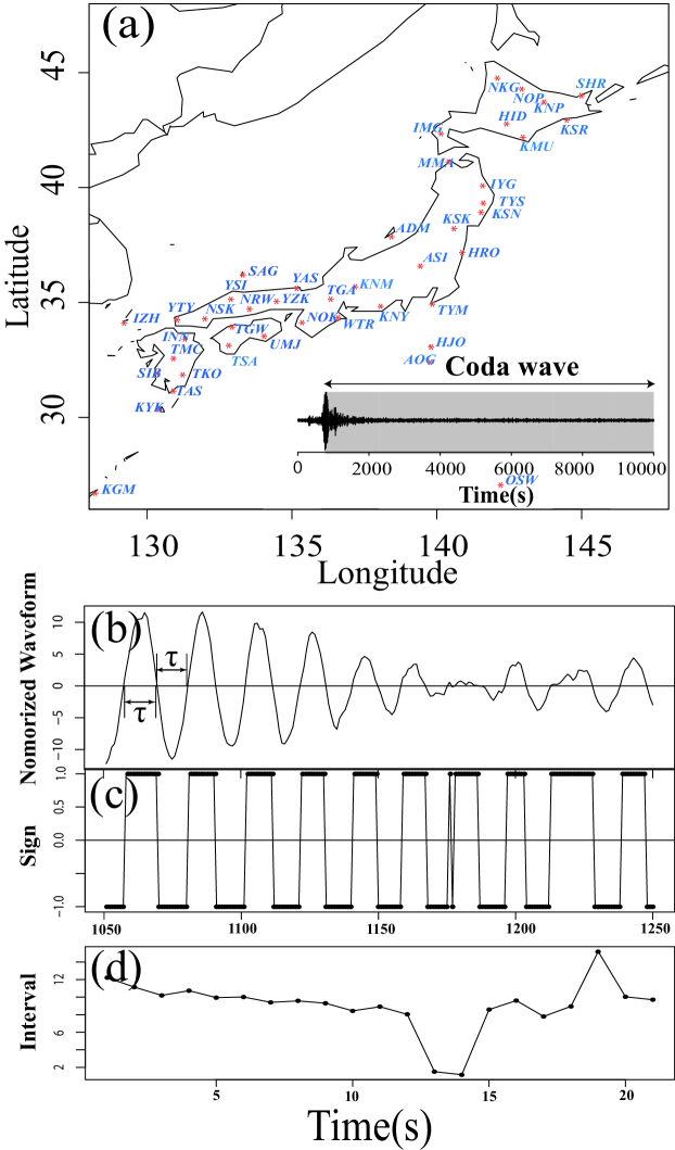
Figure 1: (a) Location map for the 46 broadband stations of Full Range Seismograph Network of Japan (F-net) (red snow marks). Inset: An example of a record of a seismic wave (Up-Down component). (b) A part of the coda wave series indicated in inset of (a), as an example. (c) An example sign time series where the positive sign (+1) represents a positive waveform, and the negative sign (-1) represents a negative waveform in coda wave series of seismic wave. (d) Interval time series ($\tau$) of the coda wave series for a subset of the record shown in (b).

Seismic waves are unique in that they have non-stationarities of a much larger order than those of any other known natural signal. Large earthquakes are characterized by a maximum amplitude that is often $>100$ times larger than the mean amplitude [see Fig. 1(a)]. This is a limitation that makes seismic waves difficult to analyze using traditional analysis. Although we might want to use detrended fluctuation analysis (DFA) CKP ; Hu ; Chen ; Chen2 , originally proposed to study the correlations in a time series in the presence of non-stationarities commonly observed in natural phenomena, the level of non-stationarity in earthquakes is so large that DFA is inappropriate regardless of the order of the polynomial fit applied Chen . Thus, due to lack of methods for highly non-stationary signals, we do not analyze correlations in the series of magnitudes, but instead analyze the correlations in the sign series [Fig. 1(c)] and interval series [Fig. 1(d)]. For our data, we use the seismic waveform database from the National Research Institute for Earth Science and Disaster Prevention (NIED) F-net (Full Range Seismograph Network of Japan), which records continuous seismic waveform data $w_{t}$ by using broadband sensors in 64 stations in Japan [see Fig. 1(a)]. In our study we select 46 stations (ADM, AOG, ASI, HID, HJO, HRO, IGK, IMG, INN, IYG, IZH, KGM, KMU, KNM, KNP, KNY, KSK, KSN, KSR, KYK, MMA, NKG, NOK, NOP, NRW, NSK, OSW, SAG, SHR, SIB, TAS, TGA, TGW, TKO, TMC, TSA, TYM, TYS, UMJ, WTR, YAS, YNG, YSI , YTY, YZK, ZMM), based on locations and integrity of data series. Seismic signals are recorded in three directions: (1) U (up-down with up positive), N (north-south with north positive), and E (east-west with east positive) Okada . In this paper, we report results from the vertical dimension only (U data), since the results for the horizontal data (N and E) data are very similar. Sampling intervals have five recording frequencies: 80Hz, 20Hz, 1Hz, 0.1Hz, and 0.01Hz. We study earthquake coda wave data with 1Hz sampling interval for the year 2003, together with selected earthquake coda wave data from 11 March 2011. We note that, because of the interaction between earthquakes, not all earthquakes can be employed in our analysis (see Appendix A). The data from 11 March 2011 is selected because it contains the notable 2011 Tohoku earthquake (“Great East Japan Earthquake”) which resulted in the tsunami that caused a number of nuclear accidents. We also add two large earthquakes ($M=7.3$ and $M=7.6$) to our study, which also occurred the same day as aftershocks.

We employ the following procedure to create our time series:

• For each selected earthquake (see Appendix A) we create a new time series, the normalized waveform denoted by $w_{t}$ out of the raw seismic acceleration waveform data

  $$w_{norm}\equiv(w_{t}-\overline{w})/\sqrt{\overline{w_{t}^{2}}-\overline{w}^{2}}.$$ (2)

• From the time series $w_{norm}$ we define a new sub-series $w_{t}^{\prime}$, starting at time coordinate where maximum $w_{t}$ occurs and terminating at the end of the normalized waveform $w_{t}^{\prime}$ (see inset in Fig1(a)).

• Let the time series $t_{i}$ denote the points in time when $w_{t}^{\prime}$ changes sign, with $t_{i}<t_{i+1}$. We define (see Fig 1(c)) the interval series by

  $$\tau_{i}\equiv t_{i}-t_{i-1}.$$ (3)

• The sign series (see Fig. 1(d)) is defined by

  $$s_{t}\equiv sgn(w_{t}^{\prime})$$ (4)

Note that our definition of interval is different than that recently defined in several papers, where the return intervals $\tau$ have studied between consecutive fluctuations above a volatility threshold $q$ in different complex systems. The probability density function (pdf) of return intervals $P_{q}(\tau)$ scales with the mean return interval as

$$P_{q}(\tau)=\overline{\tau}^{-1}f(\tau/\overline{\tau})$$ (5)

where $f()$ is a stretched exponential Yamasaki ; Wang2 ; Wang3 . Since, on average, there is one volatility above the threshold $q$ for every $\overline{\tau}_{q}$ volatilities, then it holds that BPPnas09

$$1/\overline{\tau}_{q}\approx\int_{q}^{\infty}P(|R|)d|R|=P(|R|>q)\sim q^{-\alpha}.$$ (6)

For the time intervals $\tau_{q}$ between events given by fluctuations $R$ where $R>q$ Ref. BPPnas09 derived that $\overline{\tau_{q}}$, the average of $\tau_{q}$, obeys a scaling law,

$$\overline{\tau_{q}}=q^{\alpha}$$ (7)

where by $\alpha$ denotes our estimate of the tail exponent probability density function, $P(|R|^{1+\alpha})$. Similarly, if $P(|R|)$ follows an exponential function $P(|R|)\propto\exp(-\beta|R|)$, then employing Eq. (6) we easily derive

$$\overline{\tau}_{q}\propto\exp{(\beta q)}.$$ (8)

Eq. (8) can be used as a new method for estimation of the exponential parameter $\beta$.

III Memory of interval time series

Returning to waveform data, we begin analyzing the series by studying the conditional mean

$$\langle\tau|\tau_{0}\rangle/\overline{\tau}$$ (9)

which gives the mean value of $\tau$ (see Eq. (3)) immediately following a given term $\tau_{0}$, normalized in units of $\overline{\tau}$. The conditional mean gives evidence of whether seismic memory exists in the intervals in the form of correlations or anticorrelations. For example, should correlations exist, one would expect the mean interval to be shorter in the window immediately following a small interval.

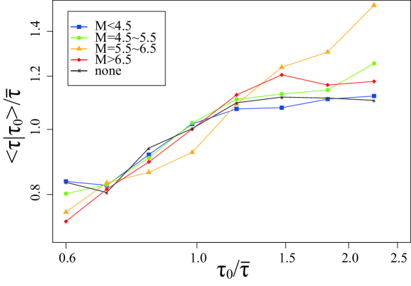
Figure 2: Scaled mean conditional interval $\langle\tau|\tau_{0}\rangle/\overline{\tau}$ vs $\tau_{0}/\overline{\tau}$ . Five groups, one with no proximal earthquake and earthquakes with Richter magnitude scale $M<4.5$, $M=4.5\sim 5.5$, $M=6.5\sim 6.5$, $M>6.5$. An increasing trend implies a short-range correlation in the interval series.

Indeed, Fig. 2 shows that the large intervals $\tau$ tend to follow large initial $\tau_{0}$ and small $\tau$ follow small $\tau_{0}$ indicating the existence of (positive) correlations in the interval time series. We also note that the autocorrelations tend to be stronger for the subset associated with larger earthquakes than for those associated with smaller earthquakes.

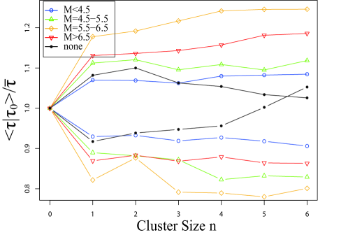
Figure 3: Long-range memory in interval clusters. $\tau_{0}$ signifies a cluster of intervals, consisting of $n$ consecutive values that all are above (denote as ”$+$”) or below (denote as ”$-$”) the median of the entire interval records. Plots display the scaled mean interval conditioned on a cluster, $\langle\tau|\tau_{0}\rangle/\overline{\tau}$ vs the size $n$ of the cluster for five group intervals. The upper part (overplotted) of curves is for ”$+$” clusters while the lower part is for ”$-$” clusters. The plots show that ”$+$” clusters are likely to be followed by large intervals and ”$-$” clusters by small intervals, consistent with long-term correlations in interval records. Similar to Fig.2, the long-term correlation increases with earthquake size, with exceptions for very large earthquakes.

To expand on this we also extend our investigation to longer range effects. We investigate the mean interval after a cluster of $n$ consecutive intervals that are either entirely above the series mean or entirely below it. We denote clusters that are entirely above the series mean with a “$+$” and clusters below the series mean with a “$-$”. Fig. 3 shows the mean interval $\tau$ that follows a $\tau_{0}(n)$ defined as a cluster size of $n$. We find that for “$+$” clusters—shown by open symbols—the mean interval increases with the size of the cluster $n$. This is the opposite of what we find for “$-$” clusters—shown as closed symbols. The results indicate the existence of at least short-term memory in the interval time series. Furthermore, we find that the mean interval increases with the seismic magnitude. However, this relationship breaks at the high end of the Richter magnitude scale $M>6.5$.

IV Detrended fluctuation analysis

Many physical, physiological, biological, and social systems are characterized by complex interactions between a large number of individual components, which manifest in scale-invariant correlations MFS ; Bunde ; Tak ; Kob82 . Since the resulting observable at each moment is the product of a magnitude and a sign, many recent investigations have focused on the study of correlations in magnitude and sign time series Ashk20 ; Kantelhardt2 ; Kant2002 ; Hu ; Plamen04itt ; Livina ; Engle82 . For example, the time series of changes $\delta\tau_{i}$ of heartbeat intervals Ashk20 ; Kant2002 ; Kantelhardt2 , physical activity levels Hu , intratrading times in the stock market Plamen04itt , and river flux values Livina all exhibit power-law anticorrelations, while their magnitudes $|\delta\tau_{i}|$ are positively correlated. A common means of finding autocorrelations hidden within a noisy non-stationary time series is detrended fluctuation analysis (DFA)CKP ; Hu ; Chen . In the DFA method, the time series is partitioned into pieces of equal size $n$. For each piece, the local trend is subtracted and the resulting standard deviation over the entire series is obtained. In general, the standard deviation $F(n)$ of the detrended fluctuations depends on $n$, with smaller $n$ resulting in trends that more closely match the data. The dependence of $F$ on $n$ can generally be represented as a power law such that

$$F(n)\propto n^{\alpha},$$ (10)

where $\alpha$ is the scaling exponent—sometimes referred to as the Hurst exponent—to be obtained empirically. DFA therefore can conceptually be understood as characterizing the motion of a random walker whose steps are given by the time series. $F(n)$ gives the walker’s deviation from the local trend as a function of the trend window. Because the root mean square displacement of a walker with no correlations between his steps scales like $\sqrt{(}n)$, we can expect a time series with no autocorrelations to yield an $\alpha$ of 0.5. Similarly, long-range power-law correlations in the signal (i.e. large terms follow large terms and small terms follow small terms) manifest as $\alpha>0.5$. Power-law anticorrelations within a signal will result in $\alpha<0.5$. Additionally, DFA can be related to the autocorrelation as follows: if the autocorrelation function $C(L)$ can be approximated by a power law with exponent $\gamma$ such that

$$C(L)\propto L^{-\gamma},$$ (11)

then $\gamma$ is related to $\alpha$ by CKP

$$\alpha\approx 1-\gamma/2.$$ (12)

Another reason we employ the DFA method is that it is appropriate for sign time series Kantelhardt2 . Other techniques for the detection of correlations in non-stationary time series are not appropriate for sign time series. Also, because the sign and interval time series have affine relations, the analysis of sign will be helpful in understanding the intervals. However, the DFA gives biased estimates for the power-law exponent in analysis of anticorrelated series Hu , and so in order to improve the accuracy of analysis, we integrate the time series before we employ the standard DFA procedure.

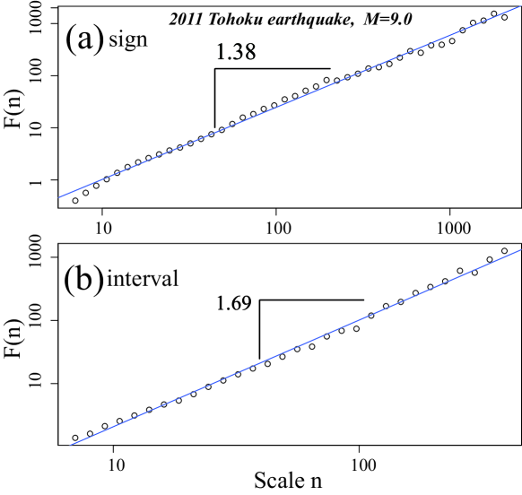
Figure 4: DFA fluctuation function $F(n)$ of 2011 Tohoku earthquake as a function of time scale $n$ ($F(n)\propto n^{\alpha}$) for (a) sign time series ($\alpha+1=1.32$, ($\alpha<0.5$), indicates anticorrelations) and (b) interval time series ($\alpha+1=1.69$, ($\alpha>0.5$), indicates correlations).

For the 2011 Tohoku earthquake, also known as the “Great East Japan Earthquake”, we present the fluctuation function $F(n)$ of the coda wave, measured at KSN station, as typical examples of sign and intervals time series (Fig. 4). By using DFA, we find, for most coda waves after earthquakes, that the time series of the intervals are consistent with a power-law correlated behavior $\alpha=0.69$, while the sign time series of Eq. (4) are consistent with a power-law anti-correlated behavior ($\alpha=0.32$). The results therefore indicate that for the interval series large increments are more likely to be followed by large increments and small increments by small increments. These results are in agreement with the results of the correlation analysis reported in Section 3. In contrast, anticorrelations in the sign time series indicate that positive increments are more likely to be followed by negative increments and vice versa.

For the entire set of sign time series comprising our sample we calculate the average DFA scaling exponent $\overline{\alpha}=0.34\pm 0.09$ indicating anticorrelations, and for the interval time series we calculate the average DFA scaling exponent $\overline{\alpha}=0.58\pm 0.08$ indicating correlations. For the different stations measuring the 2011 Tohoku earthquake we find that for the sign time series, $\overline{\alpha}=0.29\pm 0.05$ and for the interval time series, $\overline{\alpha}=0.66\pm 0.07$.

V Relation between earthquake moments and scaling exponents of sign and interval series

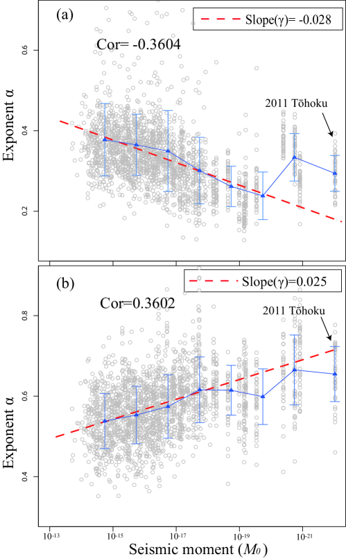
Figure 5: Scaling exponent $\alpha$ vs seismic moment (Richter magnitude scale) for (a) sign time series (correlation coefficient $Cor=-0.3604$), and (b) interval time series (correlation coefficient $Cor=0.3602$). The values of $\gamma$ show negative slope in the regression $\alpha$ vs seismic moment of the sign series, and positive slope in the regression of the interval series. Triangular symbols show the mean of exponent within each bin ( bins: $<1e+15,1e+15\sim 1e+16,1e+16\sim 1e+17,1e+17\sim 1e+18,1e+18\sim 1e+19,1e+19\sim 1e+20,>1e+21$), the error bar shows the $\pm$ standard deviation. The plots show a linear relationship between logarithmic earthquake moment and scaling exponent $\alpha$ in the sign and interval series, with exceptions for very large earthquakes.

Because large earthquake events release such extraordinary amounts of energy, it is reasonable to ask whether their occurrence influences local wave dynamics. To this end, we study interval time series of coda waves from earthquakes occurring in 2003, also including the particularly large events of 11 March 2011, when three events $M>7$ occurred in the same day. Fig. 5(a) shows the DFA scaling exponent of the sign series versus seismic moment, where seismic moment is a quantity used to measure the size of an earthquake. We find a decreasing functional dependence between the DFA exponent of the sign series and the seismic moment of the proximal earthquake with slope $\gamma=-0.028\pm 0.002$, indicating that the DFA exponent decreases approximately with seismic moment. Note that because most of the exponents are $<0.5$, this indicates the presence of ever stronger anticorrelations in the time series as earthquake magnitude increases. Note, however, that the data break with this trend for very large earthquakes (Richter magnitude scale $>6.6$ or seismic moment $>10^{19}$).

We also find similar results in the interval series, the difference being that the anticorrelations become correlations. Fig. 5(b) shows that the DFA interval exponent and seismic moment exhibit a positive functional dependence with slope $\gamma=0.025\pm 0.002$ so that the DFA exponent increases with increasing seismic moment. Because most of the exponents for the interval series are $>0.5$, this indicates that the series show stronger correlations for increasing seismic moment. Again, as with the sign series, we find a deviation from this trend for very large earthquakes.

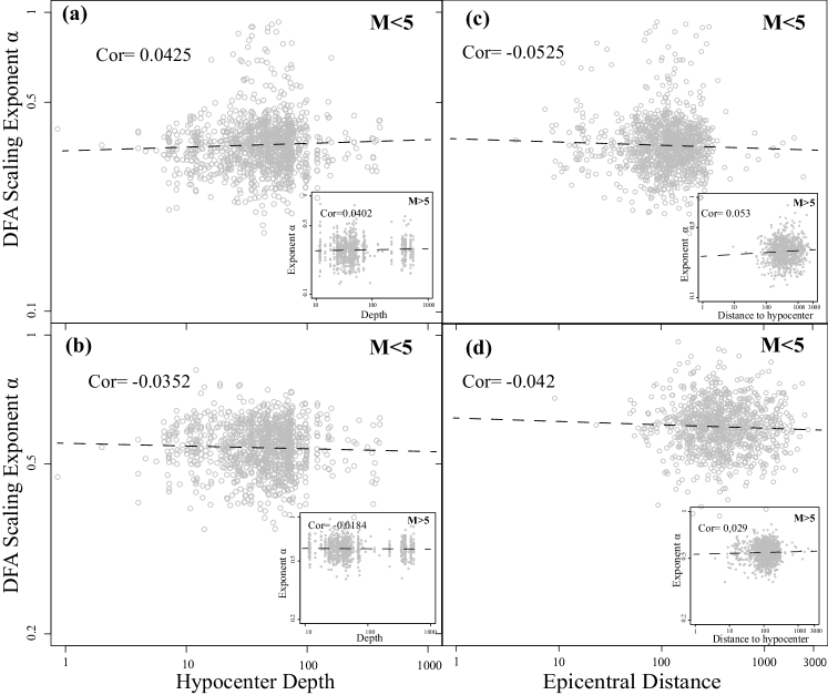
Figure 6: Scaling exponent $\alpha$ vs hypocenter depth for events where Richter magnitude scale $M<5$ for (a) sign time series (b) interval time series. Inset: scaling exponent $\alpha$ vs hypocenter depth requiring that Richter magnitude scale $M>5$. (c) and (d) show Scaling exponent $\alpha$ vs epicentral distance for events where Richter magnitude scale $M<5$. Inset: scaling exponent $\alpha$ vs epicentral distance requiring that Richter magnitude scale $M>5$. (c) sign time series, (d) interval series. All absolute values of correlation coefficient are smaller than $0.1$, showing that $\alpha$ is uncorrelated with both hypocenter depth and epicentral distance.

Having observed the influence of seismic moment on autocorrelations, we now investigate whether other readily observable factors such hypocenter depth and epicentral distance (the distance from the event to the recording station) also contribute. Specifically, we would like to explore whether there is evidence that such long-term memory is affected by the spreading process as seismic waves disseminate outward from their epicenter to a recording station or whether the memory observed is strictly due to the seismic activity. Fig. 6 shows that the DFA exponent for both interval and sign series are independent of both hypocenter depth and epicentral distance. From these results we speculate that the DFA exponent is mainly a result of the characteristics of the hypocenter rather than the process by which the seismic waves are spread.

For moderately large earthquakes ($M_{0}=10^{14}\sim 10^{19}$), we approximate the relation between the DFA scaling exponent and seismic moment through the empirical formula

$$\alpha\approx a~{}log_{10}(M_{0})+c$$ (13)

where $a=-0.028$, $c=0.797$ for the sign time series and where $a=0.025$, $c=0.174$ for the interval time series. Since

$$M=(log(M_{0})-9.1)/1.5,$$ (14)

we can also write

$$\alpha\approx a(1.5M+9.1)+c=a^{\prime}~{}M+c^{\prime},$$ (15)

where $a^{\prime}=-0.042$, $c^{\prime}=0.542$ for the sign series, and $a^{\prime}=0.037$, $c^{\prime}=0.398$ for the interval series.

We note that similar size dependence in Hurst exponent was found in Ref. Eisler where Hurst exponents of financial time series increase logarithmically with company size.

VI Summary

We analyze seismic coda waves during earthquakes, finding long-range power-law autocorrelations in both the interval and sign time series. The sign series generally display power-law anticorrelated behavior, with anticorrelations becoming stronger with larger earthquake events, while the interval series generally display power-law correlated behavior, with correlations also becoming stronger with larger earthquake events. We also show that while the DFA autocorrelation exponent is influenced by the size of the earthquake seismic moment, it is unaffected by earthquake depth or epicentral distance. Our findings are in contrast with a standard approach which assumes independence in earthquake signals and thus have strong implications on the ongoing debate about earthquake predictability SornettePNAS .

VII Acknowledgements

We thank S. Havlin for his constructive suggestions, and thank JSPS for grant of ”Research project for a sustainable development of economic and social structure dependent on the environment of the eastern coast of Asia” that made it possible to complete this study. We also thank the National Science Foundation and the Ministry of Science of Croatia for financial support.

VIII Appendix: The Selection of Earthquakes

In some regions it is common for multiple earthquakes to occur in short succession. In many cases, because the interoccurrence times are so short, the coda waves can be derived from more than one earthquake. This is especially true for large earthquakes with many aftershocks Utu . In order to make sure that the coda waves we study are the effects of only one earthquake, we need a way of determining which earthquakes are independent. We use the following two functions to determine the sphere of influence and duration of each earthquake by using the Richter magnitude scale M Utu . We select only those earthquakes that have no larger earthquake in their spatiotemporal sphere of influence,

$$t\approx 10^{(M-4.71)/1.67}$$ (16)

and

$$R\approx 2\times 10^{(M+1)/2.7},$$ (17)

where $t$ is the duration and $R$ is the sphere radius of influence. The two functions are empirical formulas based on an analysis of earthquakes in Japan Utu . The $10^{M+1.0}/2.7$ is an empirical formula that indicates the maximum radius that a human can feel an earthquake, especially for the earthquakes in Japan.

References

- (1) M. F. Shlesinger, Ann. NY Acad. Sci. 504, 214 (1987).
- (2) A. Bunde and S. Havlin (Editors), Fractals in Science (Springer, Berlin, 1994).
- (3) Y. Ashkenazy, P. C. Ivanov, S. Havlin, C. K. Peng, A. L. Goldberger, and H. E. Stanley, Phys. Rev. Lett. 86, 1900 (2001).
- (4) R. F. Engle, Econometrica 50, 987 (1982).
- (5) P. Bak, K. Christensen, L. Danon, and T. Scanlon, Phys. Rev. Lett. 88, 178501 (2002).
- (6) A. Corral, Phys. Rev. Lett. 92, 108501 (2004).
- (7) A. Corral, Phys. Rev. Lett. 95, 028501 (2005).
- (8) E. Lippiello, C. Godano, and L. de Arcangelis, Phys. Rev. Lett. 98, 098501 (2007).
- (9) Y. Y. Kagan, Bull. Seismol. Soc. Am. 94, 1207 98, 098501 (2004).
- (10) E. Lippiello, L. de Arcangelis, and C. Godano, Phys. Rev. Lett. 100, 038501 (2008).
- (11) M. Bottiglieri, L. de Arcangelis, C. Godano, and E. Lippiello, Phys. Rev. Lett. 104, 158501 (2010).
- (12) S. Lennartz, A. Bunde, and D. L. Turcotte, Geophys. J. Int. 184 1214 (2010).
- (13) V. N. Livina, S. Havlin, and A. Bunde, Phys. Rev. Lett. 95, 208501 (2005).
- (14) S. Lennartz, V. N. Livia, A. Bunde, and S. Havlin, Europhys, Lett. 81, 69001 (2008).
- (15) K. Mayeda and W. Walter, Journal of Geophysical Research 101, 11195 (1996).
- (16) Y. Hisada, Bulletin of the Seismological Society of America 90 387 (2000).
- (17) Y. Hisada, A. Shibaya, and M.R. Ghayamghamian, Bulletin Earthquake Research Institute University of Tokyo 79 81 (2004).
- (18) G. D. Bensen, M. H. Ritzwoller, M. P. Barmin, A. L. Levshin, F. Lin, M. P. Moschetti, N. M. Shapiro, and Y. Yang, Geophys. J. Int. 169, 1239 (2007).
- (19) Z. J. Xu and X. Song, Proc. Natl. Acad. Sci. USA 106, 14207 (2009).
- (20) Y. Okada, K. Kasahara, S. Hori, K. Obara, S. Sekiguchi, H. Fujiwara, and A. Yamamoto, Earth Planets Space 56, xv-xxviii (2004).
- (21) S. Ide, G. C. Beroza, D. R. Shelly, and T. Uchide, Nature 447, 76 (2007).
- (22) N. M. Shapiro, M. Campillo, L. Stehly, and M. H. Ritzwoller, Science 307, 1615 (2005).
- (23) M. Campillo and A. Paul, Science 299 547 (2003).
- (24) K. Yamasaki, A. Gozolchiani, S. Havlin, Phys. Rev. Lett. 100, 228501 (2008).
- (25) A. Gozolchiani, K. Yamasaki, O. Gazit, S. Havlin, Europhys. Lett. 83, 28005 (2008).
- (26) B. Podobnik, P. Ch. Ivanov, V. Jazbinsek, Z. Trontelj, H. E. Stanley, and I. Grosse, Phys. Rev. E Rapid Communication 71, 025104(R) (2005).
- (27) S. Lennartz, V. N. Livina, A. Bunde, and S. Havlin, Europhys. Lett. 81, 69001 (2008).
- (28) J. W. Kantelhardt, Y. Ashkenazy, P. C. Ivanov, A. Bunde, S. Havlin, T. Penzel, J. H. Peter, and H. E. Stanley, Phys. Rev. E 65, 051908 (2002).
- (29) H. E. Stanley, L. A. N. Amaral, A. L. Goldberger, S. Havlin, P. C. Ivanov, and C.K. Peng, Physica A 270, 309 (1999).
- (30) R. Karasik, N. Sapir, Y. Ashkenazy, P. C. Ivanov, I. Dvir, P. Lavie, and S. Havlin, Phys. Rev. 66, 62902 (2002).
- (31) R. Mantegna and H. E. Stanley, Nature 376, 46 (1995).
- (32) K. Yamasaki, L. Muchnik, S. Havlin, A. Bunde, and H. E. Stanley, Proc. Natl. Acad. Sci. USA 102, 9424 (2005).
- (33) F. Wang, K. Yamasaki, S. Havlin, and H. E. Stanley, Phys. Rev. E 73, 026117 (2006).
- (34) F. Wang, K. Yamasaki, S. Havlin, and H. E. Stanley, Phys. Rev. E 77, 016109 (2008).
- (35) H. E. Stanley, V. Plerou, and X. Gabaix, Physica A 387, 3967 (2008).
- (36) B. Podobnik, D. Horvatic, A. M. Petersen, and H. E. Stanley, Proc. Natl. Acad. Sci. USA 106, 22079 (2009).
- (37) B. Podobnik, D. Horvatic, A. M. Petersen, B. Urosevic, and H. E. Stanley, Proc. Natl. Acad. Sci. USA 107, 18325 (2010).
- (38) C.-K. Peng, S. V. Buldyrev, S. Havlin, M. Simons, H. E. Stanley, A. L. Goldberger, Phys. Rev. E 49, 1685 (1994).
- (39) K. Hu, P. C. Ivanov, Z. Chen, P. Carpena, H. E. Stanley, Phys. Rev. E 64, 011114 (2001).
- (40) Z. Chen, P. C. Ivanov, K. Hu, and H.E. Stanley, Phys. Rev. E 65, 041107 (2002).
- (41) Z. Chen, K. Hu, P. Carpena, P. Bernaola-Galvan, H. E. Stanley, and P. Ch. Ivanov, Phys. Rev. E 71, 011104 (2005).
- (42) H. Takayasu, Fractals in the Physical Sciences (Manchaster U. Press, Manchaster, 1997).
- (43) M. Kobayashi and T. Musha, IEEE Trans. Biomed. Eng. 29, 456 (1982).
- (44) P. Ch. Ivanov, A. Yuen, B. Podobnik, Y. Lee, Phys. Rev. E 69, 056107 (2004).
- (45) V. N. Livina, Y. Ashkenazy, P. Braun, R. Monetti, A. Bunde, S. Havlin, Phys. Rev. E 67, 042101 (2003).
- (46) J. W. Kantelhardt, S. A. Zschiegner, E. Koscielny-Bunde, S. Havlin, A. Bunde, and H. E. Stanley, Physica A 316, 87 (2002).
- (47) Z. Eisler and J. Kertesz, Eur. Phys. J. B 51, 145 (2006).
- (48) D: Sornette, Proc. Natl. Acad. Sci. USA 99, 2522 (2002).
- (49) T. Utu, Seismicity studies: a comprehensive review (University of Tokyo Press, Tokyo, 1999).