Velocity autocorrelation function of a Brownian particle

Abstract

In this article, we present molecular dynamics study of the velocity autocorrelation function (VACF) of a Brownian particle. We compare the results of the simulation with the exact analytic predictions for a compressible fluid from Chow1973 and an approximate result combining the predictions from hydrodynamics at short and long times. The physical quantities which determine the decay were determined from separate bulk simulations of the Lennard-Jones fluid at the same thermodynamic state point.We observe that the long-time regime of the VACF compares well the predictions from the macroscopic hydrodynamics, but the intermediate decay is sensitive to the viscoelastic nature of the solvent.

1 Introduction

Brownian motion is the random motion of a particle, which is large compared to the solvent molecules, but is not of macroscopic size. It has become a paradigm in various branches of science and remains an active area of research among theoreticians and experimentalists. It is not only a preferred tool of theoretical modeling, but is also extensively used to probe microscopic environments in experimentsWirtz2009 ; Squires2010 ; Frey2005 . A considerable effort is also spend in investigating transport properties of colloidal suspensions and complex fluids,primarily due to the relevance of such systems in industry, using molecular simulations of Brownian motion Vladkov2006 ; Keblinski2002 ; Padding2006 ; Lee2004 ; Eastman2004 . Such simulations always invariably involve using discrete particles to explain continuum predictions of theory, and therefore, requires a clear understanding of the molecular and continuum regimes.

In this article, using molecular dynamics simulation, we investigate the velocity autocorrelation function (VACF) of a Brownian particle. We choose a large system size so that the effect of finite-size of the simulation box is small. The internal degrees of freedom of the nanoparticle is also resolved in the simulation, such that stick boundary conditions apply on the surface of the particleLi2009 . The erratic motion of a Brownian particle exhibits a far more rich behavior than predicted by the simple Langevin picture. In the continuum description, a fluid is well described by the Stokes equation, with the particle dynamics coupled to the solvent through the imposed boundary conditions. The inadequacy of the Langevin picture in describing such erratic motion can be immediately seen from the VACF of the Brownian particle. While a simple exponential decay is predicted at all times in the Langevin model, in reality the decay exhibits distinct features of both continuum, as well as discrete nature of the solvent. Accordingly, we classify the decay in three separate regimes, a short-time regimes - where molecular nature of the solvent plays a crucial role, an intermediate regime - governed by the interplay between sound propagation, vorticity diffusion and the viscoelasticity of the solvent, and a long-time regime where the VACF decays as a power law $t^{-d/2}$ ($d$ is the dimension of space) due to the development of the slow viscous patterns in the solvent Alder1967 ; Alder1970 ; Hauge1973 ; Chow1973 ; Herschkowitz-Kaufman1972 . We compare the results from the simulations with the exact predictions from hydrodynamics, and observe, that, while the decay of the VACF at long times compares well with the predictions from hydrodynamics, the intermediate decay is sensitive to the viscoelastic nature of the fluid and can not be explained by only considering the compressible nature of the fluid.

Using a molecular dynamics simulation to investigate short and long-time dynamics of isothermal Brownian motion is a non-trivial task. The key points in such simulations, are the identification of relevant length and time scales. The two important length scales in the system are the simulation box size $L$ and the radius of the particle $R$. In a typical molecular dynamics simulation periodic boundary conditions are imposed, implying that the dynamics of the particle is effected by its periodic images. Since the strength of such finite size effect is determined by the ratio of the two length scales, $R/L$, we have the choice of a small $R$ or large $L$. Both of these choices are unfortunately restricted. While the choice of $L$ is solely determined by the computational resources at hand, the choice of $R$ is determined by a number of factors. Ideally, one would prefer a clear separation of the time scales in the simulation, in particular, the sonic time $\tau_{c}=R/c$ and the vorticity diffusion time $\tau_{\nu}=R^{2}/\nu$, both of which determine the decay of the VACF. A small choice of $R$ does not resolve these time scales properly.

The lower bound for $R$ is determined by the Knudsen number, defined as the ratio of the mean free path to the characteristic length scale of the flow – typically, the diameter of the particle. The Knudsen number decides whether a continuum or a statistical mechanics description of the system is appropriate. Besides the length scales, the time scales involved in a Brownian motion range from the order of $10^{-15}\,$s to seconds. The simulation must also be able to resolve the various time scales in the problem, the smallest of which is the collision time of solvent molecules and the largest time scale is the colloid diffusion time, over which the colloid diffuses over its own radius.

The remainder of the article is organized as follows. In sec:md_sim, we explain our molecular dynamics simulation in brief. The comparison of the simulation results with the exact prediction from the theory is done in sec:vacf_exact, and an approximate result is presented in sec:vacf_app.

2 Molecular Dynamics Simulation

In this section, we provide the details of our molecular dynamics simulation. To begin with, the natural choice of units is the Lennard–Jones reduced units, where length, time and energy in units of $\sigma$, $\tau=\sqrt{m\sigma^{2}/\epsilon}$ and $\epsilon$. Throughout the article, the numerical values of the physical quantities are given in reduced units, unless otherwise explicitly stated.

Our model system is made of a simple Brownian particle, with internal degress of freedom resolved, immersed in a Lennard–Jones solvent. The particles in the system interact via the Lennard–Jones interaction,

$$U(r)=4\epsilon\left[\left(\frac{\sigma}{r}\right)^{12}-\left(\frac{\sigma}{r}\right)^{6}\right].$$ (1)

Additionally, the nearest-neighbor interaction of the atoms in the spherical cluster of the nanoparticle is the FENE interaction,

$$U_{FENE}(r)=-\frac{1}{2}\kappa R_{0}^{2}\log\biggr{[}1-\biggr{(}\frac{r}{R_{0}}\biggr{)}^{2}\biggr{]},$$ (2)

where $\kappa=30\epsilon/\sigma^{2}$ is the spring constant and $R_{0}=1.5\sigma$. In order to keep the finite-size effects from the image particles to a reasonable value, we choose a large system size with a total of $256000$ particles. The initial configuration of the system was chosen to be a perfect FCC lattice with velocities drawn from a Boltzmann distribution. The nanoparticle was obtained from a spherical cut of the FCC lattice. For the smallest size of the nanoparticle ($R=3$) there were $177$ atoms in the cluster while for largest size of the nanoparticle ($R=5$) we have $767$ atoms in the cluster. The ratio $L/R$, which quantifies the finite-size in the system are $22.5795\,$ and $13.5409\,$ for the $R=3$ and $R=5$, respectively.

The system was first equilibrated under NPT ensemble, with the system coupled to a thermostat and barostat, at a thermodynamic pressure of $P_{0}=0.01$ and temperature $T_{0}=0.75$. For the implementation of the NPT ensemble we chose the Nóse-Hoover equations of motion as modified by MelchionnaMelchionna1993 ,

$$\mathbf{\dot{r}}_{i} = \mathbf{\dot{v}}_{i}+\alpha(\mathbf{\dot{r}}_{i}-\mathbf{R}_{0}),\phantom{1}\mathbf{\dot{p}}_{i}=\mathbf{F}_{i}-(\alpha+\gamma)(\mathbf{\dot{r}}_{i}-\mathbf{R}_{0})$$

$$\dot{\gamma} = \nu_{T}^{2}\biggr{(}\frac{T(t)}{T_{0}}-1\biggr{)},\phantom{1}\dot{\alpha}=\frac{\nu_{p}^{2}}{Nk_{B}T_{0}}V(p(t)-p),$$

$$\dot{V} = 3V\alpha.$$ (3)

The barostating variable $\alpha$ can be eliminated between the last two equations in Eq.(2), and the resulting equations are then numerically integrated using Leap-Frog integration schemeToxvaerd1993 .

The molecular dynamics simulations were implemented on Graphics Processing Units (GPU) and is similar to those of Anderson et. al. Anderson2008 and Colberg Colberg2009 , more closely resembling the later in the construction of the Verlet list. We briefly describe our implementation in the following lines.

We use the atom decomposition method in the simulation, for efficient parallel implementation of our MD code. Every particle in the simulation is assigned a thread, which is responsible for updating the coordinates and momenta of the particle. A GPU optimized cell list algorithm is used for construction of the Verlet list. For this purpose, the simulation domain is divided into cubes of size $r_{c}$, where $r_{c}$ is the cutoff length scale for the Lennard-Jones potential ($r_{c}=2.5\sigma$ in the present application). The particles were first sorted into their respective cells using the parallel radixsort algorithm Colberg2009 . To construct of the Verlet list, the entries of $26+1$ cells are copied to the shared memory. Every cell has an upper limit for the maximum number of entries, determined by the size of the shared memory on the GPU. This limitation also prevented us from simultaneously copying the particle coordinates to the shared memory. For a given particle in a cell, an iterative search is made of the neighboring cells and the particle coordinates are read from a texture array. The stability and numerical accuracy of our molecular dynamics code was verified by outputting the total energy and total momentum of the system. With an integration time-step $\delta t=0.001$, trajectories of $2\times 10^{7}$ steps (corresponding to a physical duration of $20\,$ ns) were simulated for the data points.

3 Velocity Autocorrelation Function

The long time tails in the VACF can be explained by the generalized Langevin equation,

$$\dot{\mathbf{P}}=-\frac{1}{M}\int_{0}^{t}\zeta(t-t^{\prime})\mathbf{P}(t^{\prime})+\boldsymbol{\xi}(t)$$ (4)

together with the time dependent friction coefficient $\zeta(t)$, where $\mathbf{P}$ is the momentum of the Brownian particle and $\boldsymbol{\xi}$ is the random force acting on it. Multiplying Eq.(4) by $\mathbf{P}(0)$, and taking an ensemble average, the velocity autocorrelation function for the Brownian particle becomes,

$$\dot{C}(t)=\frac{1}{M}\int_{0}^{t}\zeta(t-t^{\prime})C(t^{\prime}),$$ (5)

which, in the frequency space is written as,

$$\tilde{C}(\omega)=C(0)\left(-i\omega+\frac{\tilde{\zeta}(\omega)}{M}\right)^{-1}\equiv C(0)Y(\omega).$$ (6)

The zero-frequency limit of Eq.(6) produces the Stokes-Einstein relation $D=k_{\rm B}T/\zeta_{0}$. Transforming back to real time, the normalized VACF of the Brownian particle is given by

$$\frac{C(t)}{C(0)}=\int_{-\infty}^{\infty}\frac{\mathrm{d}\omega}{2\pi}Re[Y(\omega)]\cos(\omega t)$$ (7)

For an incompressible fluid, the frequency dependent friction coefficient is given by Hauge1973 ; Zwanzig1970 :

$$\tilde{\zeta}(\omega)=6\pi\eta_{0}R(1+R(-i\omega/\nu)^{1/2}-(i\omega R^{2}/9\nu)),$$ (8)

where, $\eta_{0}$ and $\nu$ are the steady-state dynamic and kinematic viscosities of the solvent,respectively. The square-root singularity in Eq.(8) gives rise to the power law decay of the VACF at long times. Because of the incompressibility condition, the equal-time value of the VACF suffers a discontinuity from the equipartition value of $k_{B}T/M$ to $k_{B}T/M^{*}$, with the effective mass $M^{*}$ given by $M^{*}=M+M_{f}/2$. $M_{f}$ is the mass of the displaced fluid.

In simulations, however, the discontinuity is not observed due to the finite compressibility of the fluid Zwanzig1970 ; Bakker2002 ; Chow1973 . In a compressible solvent, the sound propagation occurs with a finite speed, and the solvent surrounding the colloid is not instantly set in motion. A fraction of the energy of the Brownian particle is thus spent in creating these sound waves. To account for the compressibility effect of the solvent, we need to consider the Boussinesq force for unsteady motion in a compressible solventZwanzig1970 ; Chow1973 . For this purpose, we consider the frequency dependent friction coefficient presented in the works of Chow et. al. Chow1973 . For simplicity, we follow the notations in Chow1973 . In terms of the vorticity diffusion time $\tau_{\nu}=R^{2}/\nu$ and the sonic time $\tau_{c}=R/c$, $\tilde{\zeta}(\omega)$ is written as

$$x =i\sqrt{i\omega\tau_{\nu}},\,\,\,\,\,y=i\omega\tau_{c}\left[1-\frac{i\omega\tau_{c}^{2}}{\tau_{\nu}}\dfrac{(\mu+(4/3)\eta)}{\eta}\right]^{-1/2}$$ (9)

$$\tilde{\zeta}(\omega) =-\frac{4}{3}\pi\eta Rx^{2}[(1-y)Q+2(x-1)P],$$

where $P$ and $Q$ are functions of the dimensionless variables $x$ and $y$. We refer the readers to Chow1973 , for an explicit expression of these functions. Substituting Eq.(9) in Eq.(6), and subsequently using Eq.(7), we obtain the normalized VACF in real time.

The physical parameters which enter Eq.(9) were determined from separate molecular dynamics simulations of the bulk Lennard-Jones fluid at the same thermodynamic state point. The shear viscosity $\eta$ and the bulk viscosity $\mu$ were estimated from the off-diagonal and diagonal components of the stress tensor and using the Green-Kubo formula,

$$\eta(t)=\frac{V}{k_{B}T}\int_{0}^{t}\langle\sigma_{xy}(t^{\prime})\sigma_{xy}(0)\rangle\mathrm{d}t^{\prime}$$ (10)

$$\mu(t)=\frac{V}{k_{B}T}\int_{0}^{t}\langle\delta p(t^{\prime})\delta p(0)\rangle\mathrm{d}t^{\prime}$$ (11)

The infintie time limit of Eq.(10) and Eq.(11) provided the steady state values of the shear and bulf viscosity, $\eta_{0}$ and $\mu_{0}$, respectively. The adiabatic sound speed in the solvent was estimated from the relation

$$c^{2}=\frac{\gamma}{\rho m\chi_{T}},$$ (12)

where $\gamma$ is the ratio of the specific heats $C_{P}/C_{V}$, $\rho$ is the density of the solvent, $m$ is the mass of the solvent particles and $\chi_{T}$ is the isothermal thermal compressibility.

Before we compare the results of the molecular dynamics simulations with the predictions from hydrodynamics, the assumptions of the macroscopic theory needs to validated. The crucial assumption which enters the theory is the boundary condition on the surface of the particle. While Eq.(9) assumes a stick boundary condition on the particle surface, such an assumption may break down in a microscopic scale. To validate this we measured the friction coefficient for different radius of a rough Brownian particle. In figure 1, we show this dependence of the friction coefficient on the radius of the Brownian particle and compare it with predictions from Stokes law with stick and slip boundary condition. The reasonable agreement of the steady-state friction coefficient with the Stokes law $\zeta_{0}=6\pi\eta_{0}R$ indicates that hydrodynamic boundary conditions applicable on the surface of the sphere are those of stick boundary conditions.

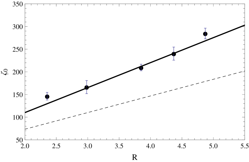
Figure 1: The dependence of the friction coefficient for different radius of the nanoparticle. The solid line is plot of Stokes law for stick boundary condition, $\zeta_{0}=6\pi\eta_{0}R$, while the dashed line shows the plot of $\zeta_{0}=4\pi\eta_{0}R$. The radius of the nanoparticle were estimated from the Eq.(14).

Additionally, the Kundsen number (Kn) for the system was determined by measuring the mean-free path of the solvent from the ballistic regime of the solvent mean-square displacement. The Knudsen number determines whether a statistical mechanics or a continuum description is more appropriate for the system and for large values of Kn (typically Kn $>0.1$), deviations from the continuum description become relevant. The measured values of Kn were $\mathrm{Kn}=0.02261$ and $\mathrm{Kn}=0.01366$, for $R=3$ and $R=5$, respectively, which indicates that the assumptions in the macroscopic hydrodynamics remains valid in the present scenario.

Moreover, due to the periodic boundary condition imposed in the simulations, the data suffers from finite-size effects from the long-ranged flow field of the image particles. We chose a sufficiently large simulation box, so that the artifact of the image particles are small. To substantiate this, we performed simualtions with two different box lengths, $L\approx 68$ and $L\approx 87$, the result of which is depicted in the Figure 2. The measured velocity autocorrelation functions does not exhibit pronounced finite-size effects, particulary in the intermediate regime of interest.

Figure 2: Velocity autocorrelation function of a Brownian particle with radius $R=5$ $(\square,\blacksquare)$ and $R=3$ ($\circ,\bullet$) for two different sizes of the simulation box, $L\approx 68$ ($\square$,$\circ$) and $L\approx 85$ ($\square$,$\bullet$).

To compare the reuslts from the simulation with the theoretical predictions for the VACF, the numerical evaluation of Eq.(7) was first carried out with the steady state values of the shear viscosity. However, we observed that the intermediate decay of the VACF can not be accurately described by only treating the solvent as compressible and it was essential to consider the viscoelastic nature of the solvent Zwanzig1970 . As already pointed out in Grimm2011 , the interaction of a colloid in a viscoelastic solvent can be visualized by considering the colloid connected to the fluid by a dash-pot and spring in series. At times larger than $\tau_{\nu}$, the viscous dissipation is represented by the dash-pot, while at shorter times the colloid interacts with the fluid via elastic forces. This caging effect is more pronounced when the ratio of the mass of the Brownian particle to the solvent particles is small Ould-Kaddour2000 . To this end, we model the Lennard-Jones solvent as Maxwell fluid with the frequency dependent viscosity given by

$$\tilde{\eta}(\omega)=\eta_{0}/(1-i\omega\tau),$$ (13)

where $\eta_{0}$ is the steady-state shear viscosity of the solvent ($\omega=0$ component). The relaxation time $\tau$ is related to the infinite frequency shear modulus $G_{\infty}$ as $\tau=\eta_{0}/G_{\infty}$. For a Lennard-Jones solvent, the single exponential relaxation in Eq.(13) ignores the algebraic decay of the stress autocorrelation at long times. This is also evident from the time dependent viscosity obtained from the simulation using Eq.(10). To illustrate this more clearly, we plot the variation of the quantity $1-\eta(t)/\eta_{0}$ with time in Fig. 3. The two distinct decays shown in Fig. 3 can be modelled as simple exponential with decay times $\tau_{1}$ and $\tau_{2}$.

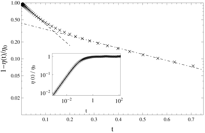
Figure 3: Decay of $1-\eta(t)/\eta_{0}$ with time. Two distinct decay-time scales are seen. At short times, comparable with molecular collision time, the decay is faster compared to the intermediate regime where power-law decay of the stress autocorrelation function becomes important. In the time-scales of interest, the decay can be modeled as simple exponential with decay time $\tau_{1}$ and $\tau_{2}$. The two time constants $\tau_{1}$ (corresponding to the dashed line) and $\tau_{2}$ (corresponding to the dot-dashed line) obtained from the above plot are $0.114$ and $0.390$, respectively. The inset shows the time dependent viscosity normalized by $\eta_{0}$.

To determine the VACF in the intermediate regime using Eq.(7) and Eq.(9) , we use $\tau_{2}$ as the relaxation time for the model fluid. Since the colloid is made of discrete number of particles, the radius of the sphere $R$ was determined from the radius of gyration using the relation

$$\langle R_{g}^{2}\rangle=\frac{1}{N}\sum_{i}^{N}(\mathbf{r}_{i}-\mathbf{R}_{\rm CM})^{2}=\frac{3}{5}R^{2}.$$ (14)

In the numerical evaluation of the VACF, we observed that the radius of the particle which gives a more accurate fit to the data was close to $R+\sigma/2$, where $\sigma$ is the diameter of the Lennard-Jones fluid particles. The values of $R$ used were $5.35$ and $3.33$ compared to the value of $R+\sigma/2=5.37$ and $R+\sigma/2=3.42$, respectively. In table 1, we compare the numerical values of the physical quantities $\eta$, $\mu$ and $c$ for a bulk Lennard-Jones fluid and those which provided the best fit to the simulated velocity autocorrelation funtion using Eq.(7) . Additionally, the mass of the colloidal particle was always taken as the reduced mass of the system.

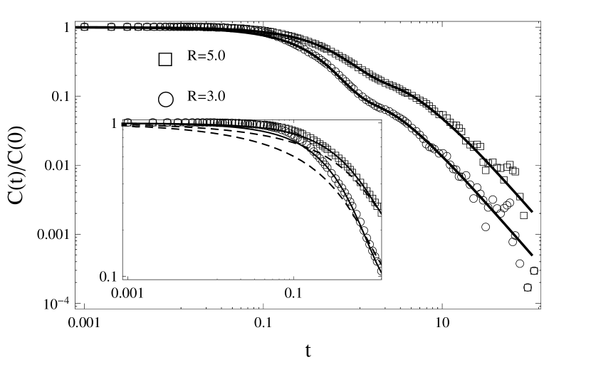
Figure 4: Decay of the velocity autocorrelation function of a Brownian particle for two particle radius $R=5$ ($\Box$) and $R=3$ ($\medcircle$). The solid-line is numerical evaluation of the normalized VACF using Eq.(7) and Eq.(9) together with a frequency dependent viscosity (Eq.(13)). The decay in the intermediate regime is sensitive to the viscoelastic nature of the solvent, and can not be accurately described using only the assumption of compressible fluid (see inset). The dashed line in the inset is the numerical evaluation with a constant viscosity.

Physical	From bulk	Value used in nu-
quantities	simulation	merical evaluation
$\eta$	$2.79961\pm 0.12963$	$2.79961$
$\mu$	$0.78556\pm 0.07442$	$0.78561$
$c$	$5.18256\pm 0.05225$	$5.15444$

Table 1: Comparison of the numerical values of the physical quantities $\eta$, $\mu$ and $c$, obtained from the bulk simulations of Lennard–Jones fluid and from best fit of the simualted VACF using Eq.(7). We note, that the values of these parameters agree within statistical error bars.

4 Approximate Result for the VACF

The inverse transformation of Eq.(7) is only possible numerically and an exact closed form analytical expression for the VACF is difficult. However, an an approximate result can be formulated using the argument of time-scale separation between $\tau_{c}$ and $\tau_{\nu}$. The sound waves created in the solvent always precedes the development of slow viscous patternsEspanol1995 , with $\tau_{c}$ usually an order of magnitude larger compared to $\tau_{\nu}$. Assuming this time scale separation, the complete decay of the VACF can be constructed by a simple addition of the VACF at short and long-time regime Padding2006 .

In the long-time regime, following Hauge1973 Paul1981 , the normalized VACF of a Browninan particle can be written as:

$$M\langle V(t)V(0)\rangle/k_{B}T=\frac{2\rho_{c}}{3\rho_{f}}\frac{1}{3\pi}\int_{0}^{\infty}\mathrm{d}x\ \frac{e^{-xt/{\tau_{\nu}}}x^{1/2}}{1+\sigma_{1}x+\sigma_{2}x^{2}}$$ (15)

with $\sigma_{1}=(1/9)(7-4\rho_{c}/\rho_{f})$ and $\sigma_{2}=(1/81)(1+2\rho_{c}/\rho_{f})^{2}$ . In Eq.(15), $\rho_{c}$ is the density of the colloid and $\rho_{f}$ is the density of the fluid. At $t=0$, the integral gives the value $\pi(1-\sqrt{\sigma_{1}^{2}-4\sigma_{2}})/\sqrt{2(\sigma_{1}-\sqrt{\sigma_{1}^{2}-4\sigma_{2}})}$, and the right-hand side of Eq.(15), after simplification, becomes $(2\rho_{c}/\rho_{f})/(1+2\rho_{c}/\rho_{f})$, producing the well known discontinuity. The discontinuity is quite easily removed when we take into account the finite compressibility of the fluid. To this end, we consider the general expression of Zwanzig Zwanzig1975 ,

$$M\langle V(t)V(0)\rangle/k_{B}T=\frac{e^{-\alpha_{1}t/\tau_{c}}}{(1+2\rho_{c}/\rho_{f})}\bigg{[}\text{Cos}\left(\frac{\alpha_{2}t}{\tau_{c}}\right)$$ (16)

$$-\frac{\alpha_{1}}{\alpha_{2}}\text{Sin}\left(\frac{\alpha_{2}t}{\tau_{c}}\right)\bigg{]}$$

with $\alpha_{1}=(1+\rho_{f}/2\rho_{c})$ and $\alpha_{2}=(1-\rho_{f}^{2}/4\rho_{c}^{2})^{1/2}$.

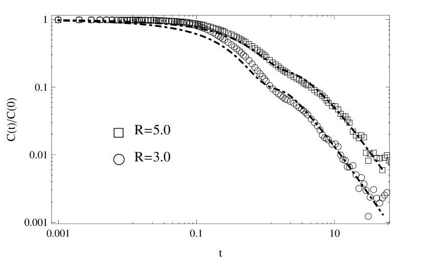
Figure 5: Comparison of the theoretical prediction of VACF with simulation for two values of the radius of the particle. The dot-dashed lines is the plot of addition of Eq.(15) and Eq.(16). Even though the fit to the simulation data is poor in the short and intermediate regime, it still reproduces the qualitative nature of the decay. The physical parameters used in the plot are the same as presented in tab:table_A

For a neutrally buoyant particle ($\rho_{c}=\rho_{f}$) the two contribution takes the form

$$\langle V(t)V(0)\rangle=\frac{2k_{B}T}{3M}\frac{1}{3\pi}\int_{0}^{\infty}\mathrm{d}x\ \frac{e^{-xt/{\tau_{\nu}}}x^{1/2}}{1+x/3+x^{2}/9}$$ (17)

and

$$\langle V(t)V(0)\rangle=\frac{K_{B}T}{3M}e^{-(3/2)(t/{\tau_{c}})}\bigg{[}\text{Cos}\bigg{(}\frac{\sqrt{3}t}{2\tau_{c}}\bigg{)}$$

$$-\sqrt{3}\text{Sin}\bigg{(}\frac{\sqrt{3}t}{2\tau_{c}}\bigg{)}\bigg{]}$$ (18)

To a first order, the complete VACF of a colloidal particle can be described by a simple addition of Eq.(17) and Eq.(4):

$$\langle V(t)V(0)\rangle=\frac{2k_{B}T}{3M}\frac{1}{3\pi}\int_{0}^{\infty}\mathrm{d}x\ \frac{e^{-xt/{\tau_{\nu}}}x^{1/2}}{1+x/3+x^{2}/9}$$

$$+\frac{K_{B}T}{3M}e^{-(3/2)(t/{\tau_{c}})}\bigg{[}\text{Cos}\bigg{(}\frac{\sqrt{3}t}{2\tau_{c}}\bigg{)}-\sqrt{3}\text{Sin}\bigg{(}\frac{\sqrt{3}t}{2\tau_{c}}\bigg{)}\bigg{]}$$

In Fig.5, we compare the normalized VACF of the Brownian particle with the theoretical predictions obtained by addition of Eq.(15) and Eq.(16).

Finally, we compare the VACF of a Brownian particle in the intermediate regime in Fig.6. The intermediate decay, between the molecular collision time and the sonic time, is clearly sensitive to the viscoelastic nature of the fluid.

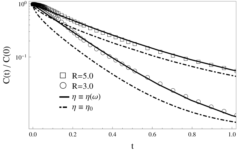
Figure 6: Comparison of the VACF of a Brownian particle in the intermediate decay regime. A reasonable fit to the data is obtained only when we consider the viscoelastic nature of the solvent. The solid line in the plot is the numerical evaluation of the VACF using a frequency dependent viscosity, and the dot-dashed lines is the plot of addition of Eq.(15) and Eq.(16).

In conclusion, using molecular dynamics simulations, we have investigated the decay of the velocity autocorrelation function (VACF) of a colloid in a Lennard-Jones solvent. The numerical values of the shear and kinematic viscosities and the speed of sound, which determine the decay, were obtained from separate simulations of the bulk Lennard-Jones fluid at the same thermodynamic state point. These values were used to determine VACF from the exact analytical prediction. Accordingly, we divide the complete decay in three regimes, a short-time regime where discrete nature of the fluid plays an important role, an intermediate regime - governed by the interplay between sound propagation, vorticity diffusion and viscoelasticity of the fluid and a long-time regime of algebraic decay due to vorticity diffusion. We observe, that the decay in the intermediate regime can not be accurately described by only considering the compressibility of the fluid, but the viscoelastic nature of the solvent should also be taken into account.

References

- (1) BJ Alder and TE Wainwright. Velocity autocorrelations for hard spheres. Physical Review Letters, 18(23):988–990, 1967.
- (2) BJ Alder and TE Wainwright. Decay of the velocity autocorrelation function. Physical review A, 1(1):18–21, 1970.
- (3) J Anderson, C Lorenz, and a Travesset. General purpose molecular dynamics simulations fully implemented on graphics processing units. Journal of Computational Physics, 227(10):5342–5359, May 2008.
- (4) A. F. Bakker and C. P. Lowe. The role of sound propagation in concentrated colloidal suspensions. The Journal of Chemical Physics, 116(13):5867, 2002.
- (5) TS Chow and JJ Hermans. Effect of inertia on the Brownian motion of rigid particles in a viscous fluid. The Journal of Chemical Physics, 56(5):3150, 1972.
- (6) TS Chow and JJ Hermans. Brownian motion of a spherical particle in a compressible fluid. Physica, 65:156–162, 1973.
- (7) PH Colberg and Felix Höfling. Accelerating glassy dynamics using graphics processing units. Arxiv preprint arXiv:0912.3824, pages 1–18, 2009.
- (8) J.a. Eastman, S.R. Phillpot, S.U.S. Choi, and P. Keblinski. Thermal Transport in Nanofluids. Annual Review of Materials Research, 34(1):219–246, August 2004.
- (9) P Espanol. On the propagation of hydrodynamic interactions. Physica A: Statistical and Theoretical Physics, 214(2):185–206, March 1995.
- (10) E. Frey and K. Kroy. Brownian motion: a paradigm of soft matter and biological physics. Annalen der Physik, 14(1-3):20–50, February 2005.
- (11) Matthias Grimm, Sylvia Jeney, and Thomas Franosch. Brownian motion in a Maxwell fluid. Soft Matter, 7(5):2076, 2011.
- (12) E. H. Hauge and A. Martin-Löf. Fluctuating hydrodynamics and Brownian motion. Journal of Statistical Physics, 7(3):259–281, March 1973.
- (13) P Keblinski, SR Phillpot, and SUS Choi. Mechanisms of heat flow in suspensions of nano-sized particles (nanofluids). of Heat and Mass Transfer, 45(4):855–863, February 2002.
- (14) Song Hi Lee and Raymond Kapral. Friction and diffusion of a Brownian particle in a mesoscopic solvent. The Journal of chemical physics, 121(22):11163–9, December 2004.
- (15) Zhigang Li. Critical particle size where the Stokes-Einstein relation breaks down. Physical Review E, 80(6):061204, December 2009.
- (16) Simone Melchionna, Giovanni Ciccotti, and Brad Lee Holian. Hoover NPT dynamics for systems varying in shape and size. Molecular Physics, 78(3):533–544, February 1993.
- (17) F. Ould-Kaddour and D. Levesque. Molecular-dynamics investigation of tracer diffusion in a simple liquid: Test of the Stokes-Einstein law. Physical Review E, 63(1):1–9, December 2000.
- (18) J. Padding and A. Louis. Hydrodynamic interactions and Brownian forces in colloidal suspensions: Coarse-graining over time and length scales. Physical Review E, 74(3):1–29, September 2006.
- (19) G L Paul and P N Pusey. Observation of a long-time tail in Brownian motion. Journal of Physics A: Mathematical and General, 14(12):3301–3327, December 1981.
- (20) Todd M. Squires and Thomas G. Mason. Fluid Mechanics of Microrheology. Annual Review of Fluid Mechanics, 42(1):413–438, January 2010.
- (21) S Toxvaerd. Molecular dynamics at constant temperature and pressure. Physical Review E, 47(1):343–350, 1993.
- (22) Mihail Vladkov and Jean-Louis Barrat. Modeling transient absorption and thermal conductivity in a simple nanofluid. Nano letters, 6(6):1224–8, June 2006.
- (23) Denis Wirtz. Particle-tracking microrheology of living cells: principles and applications. Annual review of biophysics, 38:301–26, January 2009.
- (24) R Zwanzig and M Bixon. Hydrodynamic theory of the velocity correlation function. Physical Review A, 1970.
- (25) Robert Zwanzig and Mordechai Bixon. Compressibility effects in the hydrodynamic theory of Brownian motion. Journal of Fluid Mechanics, 69(01):21–25, March 1975.