The Wang–Landau algorithm reaches the flat histogram criterion in finite time

Abstract

The Wang–Landau algorithm aims at sampling from a probability distribution, while penalizing some regions of the state space and favoring others. It is widely used, but its convergence properties are still unknown. We show that for some variations of the algorithm, the Wang–Landau algorithm reaches the so-called flat histogram criterion in finite time, and that this criterion can be never reached for other variations. The arguments are shown in a simple context—compact spaces, density functions bounded from both sides—for the sake of clarity, and could be extended to more general contexts.

and nusSupported in part by AXA research. gisSupported in part by a GIS Sciences de la Décision postdoc scholarship.

1 Introduction and notation

Consider the problem of sampling from a probability distribution $\pi$ defined on a measure space $(\mathcal{X},\Sigma,\mu)$. We suppose that we can compute the probability density function of $\pi$ at any point $x\in\mathcal{X}$, up to a multiplicative constant. Given a proposal kernel $Q(\cdot,\cdot)$ we define a Metropolis–Hastings (MH) [Hastings (1970), Tierney (1998)] transition kernel targeting $\pi$, denoted by $K(\cdot,\cdot)$, as follows:

$$\forall x,y\in\mathcal{X}\qquad K(x,y)=Q(x,y)\rho(x,y)+\delta_{x}(y)\bigl{(}1-r(x)\bigr{)}$$

with $\rho(x,y)$ defined by $\rho(x,y):=1\wedge\frac{\pi(y)}{\pi(x)}\frac{Q(y,x)}{Q(x,y)}$ and $r(x)$ defined by

$$r(x):=\int_{\mathcal{X}}\rho(x,y)Q(x,y)\,dy.$$

Here the delta function $\delta_{a}(b)$ takes value $1$ when $a=b$ and $0$ otherwise. Under some conditions on the proposal $Q$ and the target $\pi$, the MH kernel defines an algorithm to generate a Markov chain with stationary distribution $\pi$ [Robert and Casella (2004)].

Let us consider a partition of the state space $\mathcal{X}$ into $d$ disjoint sets $\mathcal{X}_{1},\ldots,\mathcal{X}_{d}$,

$$\mathcal{X}=\bigcup_{i=1}^{d}\mathcal{X}_{i}.$$

If we have a sample $X_{1},\ldots,X_{t}$ independent and identically distributed from $\pi$, then for any $i\in[1,d]$,

$$\frac{1}{t}\sum_{n=1}^{t}\mathbh{1}_{\mathcal{X}_{i}}(X_{n})\mathop{\longrightarrow}^{\mathbb{P}}_{t\to\infty}\int_{\mathcal{X}_{i}}\pi(x)\,dx=:\psi_{i},$$

where we denote by $\mathbh{1}_{\mathcal{X}_{i}}(x)$ the indicator function that is equal to $1$ when $x\in\mathcal{X}_{i}$ and $0$ otherwise. Similar convergence is obtained when $X_{1},\ldots,X_{t}$ is an ergodic chain such as the one generated by the MH algorithm. The purpose of the Wang–Landau algorithm [Wang and Landau (2001a, 2001b), Liang (2005), Atchadé and Liu (2010)] is to obtain a sample:

• such that for any $i\in[1,d]$, the subsample

  $$\bigl{\{}X_{n}\mbox{ for }n\in[1,t]\mbox{ s.t. }X_{n}\in\mathcal{X}_{i}\bigr{\}}$$

  is distributed according to the restriction of $\pi$ to $\mathcal{X}_{i}$, and

• such that for any $i\in[1,d]$,

  $$\frac{1}{t}\sum_{n=1}^{t}\mathbh{1}_{\mathcal{X}_{i}}(X_{n})\mathop{\longrightarrow}^{\mathbb{P}}_{t\to\infty}\phi_{i},$$

  where $\phi=(\phi_{1},\ldots,\phi_{d})$ is chosen by the user, and could be any vector in $]0,1[^{d}$ such that $\sum_{i=1}^{d}\phi_{i}=1$.

A typical use of this algorithm is to sample from multimodal distributions, by penalizing already-visited regions and favoring the exploration of regions between modes, in an attempt to recover all the modes. In many applications, $\phi$ is set to $\forall i,\phi_{i}=1/d$; however, other choices are possible, as exemplified by the adaptive binning scheme of Bornn et al. (2011).

This algorithm, in the class of Markov chain Monte Carlo (MCMC) algorithms [Robert and Casella (2004)], therefore allows us to learn about $\pi$ while “forcing” the proportions of visits $\phi_{i}$ of the generated chain to any of the sets $\mathcal{X}_{i}$, which are typically also chosen by the user. The vector $\phi_{1},\ldots,\phi_{d}$ might be referred to as the “desired frequencies,” and the sets $\mathcal{X}_{i}$ are called the “bins.” In a typical situation, the mass of $\pi$ over bin $\mathcal{X}_{i}$, which we denote by $\psi_{i}$, is unknown, and hence one cannot easily guess how much to “penalize” or to “favor” a bin $\mathcal{X}_{i}$ in order to obtain the desired frequency $\phi_{i}$. The Wang–Landau algorithm introduces a vector $\theta_{t}=(\theta_{t}(1),\ldots,\theta_{t}(d))$, referred to as “penalties” at time $t$, which is updated at every iteration $t$, and which acts like an approximation of the ratios $\psi_{1}/\phi_{1},\ldots,\psi_{d}/\phi_{d}$, up to a multiplicative constant.

For a distribution $\pi$ and a vector of penalties $\theta=(\theta(1),\ldots,\theta(d))$, we define the penalized distribution $\pi_{\theta}$,

$$\pi_{\theta}(x)\propto\pi(x)\times\sum_{i=1}^{d}\frac{\mathbh{1}_{\mathcal{X}_{i}}(x)}{\theta(i)}.$$

To be more concise we define a function $J\dvtx\mathcal{X}\mapsto\{1,\ldots,d\}$ that takes a state $x\in\mathcal{X}$ and returns the index $i$ of the bin $\mathcal{X}_{i}$ such that $x\in\mathcal{X}_{i}$. We can now write $\pi_{\theta}(x)\propto\pi(x)/\theta(J(x))$. We will denote by $K_{\theta}$ the MH kernel targeting $\pi_{\theta}$.

The Wang–Landau algorithm, described in the next section, alternates between generating a sample by targeting $\pi_{\theta}$ using $K_{\theta}$, and updating $\theta$ using the generated sample. In this sense it is an adaptive MCMC algorithm (past samples are used to update the kernel at a given iteration), using an auxiliary chain $(\theta_{t})$, and therefore the behavior of the sample is not obvious.

The Wang–Landau algorithm is widely used in the Physics community [Silva, Caparica and Plascak (2006), Malakis, Kalozoumis and Tyraskis (2006), Cunha Netto et al. (2006)]. In particular, many practitioners use flavors of the algorithm with a “flat histogram” criterion. However, its convergence properties are still partially unknown. We show that this criterion is reached in finite time for some variations of the algorithm. This result is all that was missing to apply results on adaptive algorithms with diminishing adaptation [Fort et al. (2011)].

In Section 2, we define variations of the Wang–Landau algorithm. We then introduce ratios of penalties and argue for their convenience in studying the properties of the algorithm. We prove in Sections 3 and 4 that under certain conditions, the flat histogram criterion is met in finite time, for the cases $d=2$ and $d>2$, respectively. The result is illustrated in Section 5, and in Section 6, we hint at how our assumptions might be relaxed.

2 Wang–Landau algorithms: Different flavors

There are several versions of the Wang–Landau algorithm. We describe the general version introduced by Atchadé and Liu (2010), both in its deterministic form and with a stochastic schedule.

2.1 A first version with deterministic schedule

Let $(\gamma_{t})_{t\in\mathbb{N}}$ (referred to as a schedule or a temperature) be a sequence of positive real numbers such that

$$\cases{\displaystyle\sum_{t\geq 0}\gamma_{t}=\infty,\vspace*{2pt}\cr\displaystyle\sum_{t\geq 0}\gamma_{t}^{2}<\infty.}$$

A typical choice is $\gamma_{t}:=t^{-\alpha}$ with $\alpha\in\,]0.5,1[$. The Wang–Landau algorithm is described in pseudo-code in Algorithm 1. In this form, the schedule $\gamma_{t}$ decreases at each iteration, and is therefore called “deterministic.”

Algorithm 1 Wang–Landau with deterministic schedule.

1:  Init $\forall i\in\{1,\ldots,d\}$ set $\theta_{0}(i)\leftarrow 1/d$.

2:  Init $X_{0}\in\mathcal{X}$.

3:  for $t=1$ to $T$ do

4:     Sample $X_{t}$ from $K_{\theta_{t-1}}(X_{t-1},\cdot)$, MH kernel targeting $\pi_{\theta_{t-1}}$.

5:      Update the penalties: $\log\theta_{t}(i)\leftarrow\log\theta_{t-1}(i)+f(\mathbh{1}_{\mathcal{X}_{i}}(X_{t}),\phi_{i},\gamma_{t})$.

6:  end for

Step 5 of Algorithm 1 updates the penalties from $\theta_{t-1}$ to $\theta_{t}$, by increasing it if the corresponding bin has been visited by the chain at the current iteration, and by decreasing it otherwise. This rationale seems natural; however, we did not find any article arguing for a particular choice of update, among the infinite number of updates that would also follow the same rationale. In other words, it is not obvious how to choose the function $f$, except that it should be such that it is positive when $X_{t}\in\mathcal{X}_{i}$ and such that it is closer to $0$ when $\gamma_{t}$ decreases, to ensure that the penalties converge. Some practitioners use the following update:

$$\log\theta_{t}(i)\leftarrow\log\theta_{t-1}(i)+\gamma_{t}\bigl{(}\mathbh{1}_{\mathcal{X}_{i}}(X_{t})-\phi_{i}\bigr{)}$$ (1)

while others use

$$\log\theta_{t}(i)\leftarrow\log\theta_{t-1}(i)+\log\bigl{[}1+\gamma_{t}\bigl{(}\mathbh{1}_{\mathcal{X}_{i}}(X_{t})-\phi_{i}\bigr{)}\bigr{]}.$$ (2)

Since $\gamma_{t}$ converges to $0$ when $t$ increases, and since update (1) is the first-order Taylor expansion of update (2), one legitimately expects both updates to result in similar performance in practice. We shall see in Section 3 that this is not necessarily the case.

Some convergence results have been proven about Algorithm 1: the deterministic schedule ensures that $\theta_{t}$ changes less and less along the iterations of the algorithm, and consequently the kernels $K_{\theta_{t}}$ change less and less as well. The study of the algorithm hence falls into the realm of adaptive MCMC where the diminishing adaptation condition holds [Andrieu and Thoms (2008), Atchadé et al. (2009), Fort et al. (2011)], although it is original in the sense that the target distribution, ($\pi_{\theta_{t}}$) is adaptive, but not necessarily the proposal distribution $Q$. See also the literature on stochastic approximation, Andrieu, Moulines and Priouret (2005).

In this article we are especially interested in a more sophisticated version of the Wang–Landau algorithm that uses a stochastic schedule, and for which, as we shall see in the following, the two updates result in different performance.

2.2 A sophisticated version with stochastic schedule

A remarkable improvement has been made over Algorithm 1: the use of a “flat histogram” (FH) criterion to decrease the schedule only at certain random times. Let us introduce $\nu_{t}(i)$, the number of generated points at iteration $t$ that are in $\mathcal{X}_{i}$,

$$\nu_{t}(i):=\sum_{n=1}^{t}\mathbh{1}_{\mathcal{X}_{i}}(X_{n}).$$

For some predefined precision threshold $c$, we say that FH is met at iteration $t$ if

$$\max_{i\in\{1,\ldots,d\}}\biggl{|}\frac{\nu_{t}(i)}{t}-\phi_{i}\biggr{|}<c.$$

Intuitively, this criterion is met if the observed proportion of visits to each bin is not far from $\phi$, the desired proportion. The name “flat histogram” comes from the observation that if the desired proportions are all equal to $1/d$, this criterion is verified when the histogram of visits is approximately flat. The threshold $c$ could possibly decrease along the iterations to get an always finer precision.

The Wang–Landau with flat histogram (Algorithm 2) is similar to the previous algorithm, with a single difference: the schedule $\gamma$ does not decrease at each step anymore, but only when FH is met. To know whether it is met or not, a counter $\nu_{t}$ of visits to each bin is updated at each iteration, and when FH is met, the schedule decreases and the counter is reset to $0$.

Algorithm 2 Wang–Landau with flat histogram

1:  Init $\forall i\in\{1,\ldots,d\}$ set $\theta_{0}(i)\leftarrow 1/d$.

2:  Init $X_{0}\in\mathcal{X}$.

3:  Init $\kappa=0$, the number of FH criteria already reached.

4:  Init the counter $\forall i\in\{1,\ldots,d\}\ \nu_{1}(i)\leftarrow 0$

5:  for $t=1$ to $T$ do

6:     Sample $X_{t}$ from $K_{\theta_{t-1}}(X_{t-1},\cdot)$ targeting $\pi_{\theta_{t-1}}$.

7:     Update $\nu_{t}$: $\forall i\in\{1,\ldots,d\}\ \nu_{t}(i)\leftarrow\nu_{t-1}(i)+\mathbh{1}_{\mathcal{X}_{i}}(X_{t})$

8:     Check whether FH is met.

9:     if FH is met then

10:        $\kappa\leftarrow\kappa+1$

11:        $\forall i\in\{1,\ldots,d\}\ \nu_{t}(i)\leftarrow 0$

12:     end if

13:      Update the bias: $\log\theta_{t}(i)\leftarrow\log\theta_{t-1}(i)+f(\mathbh{1}_{\mathcal{X}_{i}}(X_{t}),\phi_{i},\gamma_{\kappa})$.

14:  end for

Note the difference between Algorithms 1 and 2: $\gamma$ is indexed by $\kappa$ instead of $t$, and $\kappa$ is a random variable. As with Algorithm 1, the update of penalties (step 13 of Algorithm 2) can be either update (1) or update (2), or possibly something else. Interestingly in this case, it is not obvious anymore that both updates will give similar results. Indeed, for $\gamma_{\kappa}$ to go to $0$, we need FH to be reached in finite time, so that $\kappa$ regularly increases.

This flavor of the Wang–Landau algorithm is widely used in the Physics literature [Cunha Netto et al. (2006), Silva, Caparica and Plascak (2006), Malakis, Kalozoumis and Tyraskis (2006), Ngo and Diep (2008)].

Our contribution is to show in a simple context that update (1) is such that FH is met in finite time, while (2) is not so. Hence only using update (1) can one expect the convergence properties of Algorithm 1 to still hold for Algorithm 2, since if FH is met in finite time, a sort of diminishing adaptation condition would still hold.

To underline the difficulty of knowing whether FH is met in finite time or not, let us recall that between two FH occurrences, the schedule is constant (equal to some $\gamma_{\kappa}>0$); hence the penalties $(\theta_{t})$ change at a constant scale and diminishing adaptation does not directly hold. Other adaptive algorithms share this lack of diminishing adaptation, as, for example, the accelerated stochastic approximation algorithm [Kesten (1958)], in which the adaptation of some process diminishes only if its increments change sign. In our case, FH will be reached if the chain $(X_{t})$ lands with frequency $\phi_{i}$ in each bin $\mathcal{X}_{i}$; see Corollary 2.

Note that in the implementation of the algorithm, the penalties $\theta_{t}$ need only be defined up to a normalizing constant, since they only appear in ratios of the form $\theta_{t}(i)/\theta_{t}(j)$. We therefore introduce the following notation:

$$\forall i,j\in\{1,\ldots,d\}\mbox{ such that }i\neq j\qquad Z_{t}^{(i,j)}=\log\frac{\theta_{t}(i)}{\theta_{t}(j)},$$

and we note $Z_{t}$ the collection of all the $Z_{t}^{(i,j)}$. Some intuition behind the study of such ratios comes from considering update (1). With this update, assume that for each $i$, $\mathbb{E}[\mathbh{1}_{\mathcal{X}_{i}}(X_{t})]=\phi_{i}$. Then we could easily check that for each pair $(i,j)$, $\mathbb{E}[Z_{t}^{(i,j)}|Z_{t-1}^{(i,j)}]=Z_{t-1}^{(i,j)}$, so this process would be constant on average. The remainder of this paper hinges on two facts: that we can control $(Z_{t})$ in the sense that $Z_{t}^{(i,j)}/t\to 0$, and that if we control $(Z_{t})$, then we control the frequencies of visits $(\nu_{t}/t)$.

More generally, notice that with fixed $\gamma$, the pair $(X_{t},Z_{t})$ forms a homogeneous Markov chain. We would like to prove that its proportion of visits to the set $\mathcal{X}_{i}\times\mathbb{R}^{d(d-1)}$ converges to some value in $[0,1]$; one way to prove this is to show that the chain is irreducible. We would then need to check that the limit is indeed the desired frequency $\phi_{i}$ for all $i$. Unfortunately, properties of the joint chain $(X_{t},Z_{t})$ are difficult to establish due to the complexity of its transition kernel. Finding a so-called drift function for the joint Markov chain is also typically difficult. In general, we are not able to show that the chain is irreducible. In Section 3, we prove directly that $Z_{t}^{1,2}/t\to 0$ in the special case $d=2$, under some assumptions. In Section 4, we make more restrictive assumptions which imply irreducibility. In both cases, we show the implication of this convergence on the frequencies of visits.

3 Proof when $d=2$

In the following we consider a simple context with only two bins: $d=2$ and $X_{t}$ can therefore only be either in $\mathcal{X}_{1}$ or in $\mathcal{X}_{2}$. Suppose the current schedule is at $\gamma>0$, and we want to know whether FH is going to be met in finite time (hence $\gamma$ is fixed here). To simplify notation, in this section we note

$$Z_{t}=Z_{t}^{(1,2)}=\log\theta_{t}(1)-\log\theta_{t}(2).$$

Using the definition of the penalties $(\theta_{t})$ and of the counts $(\nu_{t})$, we obtain

$$Z_{t} = Z_{0}+\bigl{[}\nu_{t}(1)f(1,\phi_{1},\gamma)+\bigl{(}t-\nu_{t}(1)\bigr{)}f(0,\phi_{1},\gamma)\bigr{]}$$

$${}-\bigl{[}\nu_{t}(2)f(1,\phi_{2},\gamma)+\bigl{(}t-\nu_{t}(2)\bigr{)}f(0,\phi_{2},\gamma)\bigr{]}$$

$$= Z_{0}+\nu_{t}(1)\bigl{[}f(1,\phi_{1},\gamma)-f(0,\phi_{1},\gamma)\bigr{]}+tf(0,\phi_{1},\gamma)$$

$${}-\bigl{[}\bigl{(}t-\nu_{t}(1)\bigr{)}f(1,\phi_{2},\gamma)+\nu_{t}(1)f(0,\phi_{2},\gamma)\bigr{]}$$

$$= Z_{0}+\nu_{t}(1)\bigl{[}f(1,\phi_{1},\gamma)-f(0,\phi_{1},\gamma)+f(1,\phi_{2},\gamma)-f(0,\phi_{2},\gamma)\bigr{]}$$

$${}+t\bigl{(}f(0,\phi_{1},\gamma)-f(1,\phi_{2},\gamma)\bigr{)}.$$

If we prove that $Z_{t}/t$ goes to $0$ (e.g., in mean), this will imply the following convergence of the proportion of visits:

$$\frac{\nu_{t}(1)}{t}\mathop{\longrightarrow}_{t\to\infty}\frac{f(1,\phi_{2},\gamma)-f(0,\phi_{1},\gamma)}{f(1,\phi_{1},\gamma)-f(0,\phi_{1},\gamma)+f(1,\phi_{2},\gamma)-f(0,\phi_{2},\gamma)}$$

(also in mean). Since we want FH to be reached in finite time for any precision threshold $c>0$, we need the proportions of visits to $\mathcal{X}_{i}$ to converge to $\phi_{i}$. Hence we want

$$\frac{f(1,\phi_{2},\gamma)-f(0,\phi_{1},\gamma)}{f(1,\phi_{1},\gamma)-f(0,\phi_{1},\gamma)+f(1,\phi_{2},\gamma)-f(0,\phi_{2},\gamma)}=\phi_{1}.$$ (3)

Using the specific forms of $f(\mathbh{1}_{\mathcal{X}_{i}}(X_{t}),\phi_{i},\gamma)$ for both updates, we can easily see that:

• update (1) satisfies equation (3) for any $\phi$ and $\gamma$;

• in general, update (2) does not satisfy equation (3), except in the special case where $\phi_{1}=\phi_{2}=1/2$.

Note that the second point states that the proportions of visits converge to some vector $\tilde{\phi}$ different than $\phi$. The vector $\tilde{\phi}$ can be expressed as a function of $\phi\dvtx\tilde{\phi}=g(\phi)$. By numerically or analytically inverting this function $g$, one can plug $g^{-1}(\phi)$ as an algorithmic parameter, so that the limiting proportions of visits converge to $g(g^{-1}(\phi))=\phi$. Hence one can use update (2) and get the desired proportions of visits by plugging $g^{-1}(\phi)$ instead of $\phi$ in the update.

The rest of the paper is devoted to the proof that $Z_{t}/t$ goes to $0$ under some assumptions. More formally, we state in Theorem 1 what we shall prove in the remainder of this section. This theorem holds for both updates.

Theorem 1

Consider the sequence of penalties $(\theta_{t})$ introduced in Algorithm 2. We define

$$Z_{t}=\log\theta_{t}(1)-\log\theta_{t}(2).$$

Then

$$\frac{Z_{t}}{t}\mathop{\longrightarrow}^{L_{1}}_{t\to\infty}0.$$

As a consequence, the long run proportion of visits to each bin converges to the desired frequency $\phi$ for update (1), and not necessarily for update (2). Corollary 2 clarifies the consequence of Theorem 1 on the validity of Algorithm 2.

Corollary 2.

When the proportions of visits converge in mean to the desired proportions, the flat histogram criterion is reached in finite time for any precision threshold $c$.

We already made the simplification of considering the simple case $d=2$. We make the following assumptions:

Assumption 1.

The bins are not empty with respect to $\mu$ and $\pi$,

$$\forall i\in\{1,2\}\qquad\mu(\mathcal{X}_{i})>0\quad\mbox{and}\quad\pi(\mathcal{X}_{i})>0.$$

Assumption 2.

The state space $\mathcal{X}$ is compact.

Assumption 3.

The proposition distribution $Q(x,y)$ is such that

$$\exists q_{\mathrm{min}}>0\ \forall x\in\mathcal{X}\ \forall y\in\mathcal{X}\qquad Q(x,y)>q_{\mathrm{min}}.$$

Assumption 4.

The MH acceptance ratio is bounded from both sides

$$\exists m>0\ \exists M>0\ \forall x\in\mathcal{X}\ \forall y\in\mathcal{X}\qquad m<\frac{\pi(y)}{\pi(x)}\frac{Q(y,x)}{Q(x,y)}<M.$$

Assumption 1 guarantees that the bins are well designed, and if it was not verified, the algorithm would never reach FH, regardless of the other assumptions. Assumptions 2–4 are, for example, verified by a Gaussian random walk proposal over a compact space, where there is a lower bound on $\pi$. We believe that these assumptions can be relaxed to cover the most general Wang–Landau algorithm. Making these four assumptions allows us to propose a clearer proof, and we propose hints on how to relax them in Section 6.

We denote by $U_{t}$ the increment of $Z_{t}$, such that for any $t$,

$$Z_{t+1}=Z_{t}+U_{t}=Z_{t}+f\bigl{(}\mathbh{1}_{\mathcal{X}_{1}}(X_{t}),\phi_{1},\gamma\bigr{)}-f\bigl{(}\mathbh{1}_{\mathcal{X}_{2}}(X_{t}),\phi_{2},\gamma\bigr{)}.$$

Here with only two bins, the increments $U_{t}$ can take two different values, $+a$ or $-b$, for some $a>0$ and $b>0$ that depend on $\phi$ and $\gamma$. For example, with update (1),

$$\cases{a=2\gamma(1-\phi_{1})>0,\vspace*{2pt}\cr b=2\gamma\phi_{1}>0,}$$

whereas with update (2),

$$\cases{\displaystyle a=\log\biggl{(}\frac{1+\gamma(1-\phi_{1})}{1-\gamma(1-\phi_{1})}\biggr{)}>0,\vspace*{2pt}\cr\displaystyle b=\log\biggl{(}\frac{1+\gamma\phi_{1}}{1-\gamma\phi_{1}}\biggr{)}>0,}$$

and in both cases, if $X_{t}\in\mathcal{X}_{1}$, then $U_{t}=+a$, otherwise $U_{t}=-b$.

We want to prove that $Z_{t}/t$ goes to $0$, and we are going to prove a stronger result that states, in words, that when $Z_{t}$ leaves a fixed interval $[\bar{Z}^{\mathrm{lo}},\bar{Z}^{\mathrm{hi}}]$, it returns to it in a finite time.

3.1 Behavior of $(Z_{t})$ outside an interval

First, Lemma 3 states that if $Z_{t}$ goes above a value $\bar{Z}^{\mathrm{hi}}$, it has a strictly positive probability of starting to decrease, and that when that happens, it keeps on decreasing with a high probability.

Lemma 3

With the introduced processes $Z_{t}$ and $U_{t}$, there exists $\epsilon>0$ such that for all $\eta>0$, there exists $\bar{Z}^{\mathrm{hi}}$ such that, if $Z_{t}\geq\bar{Z}^{\mathrm{hi}}$, we have the following two inequalities:

$$P[U_{t+1}=-b|U_{t}=+a,Z_{t}] > \epsilon,$$

$$P[U_{t+1}=-b|U_{t}=-b,Z_{t}] > 1-\eta.$$

We start with the first inequality. Let $q_{\mathrm{min}}$ be like in Assumption 3.

In terms of events $\{U_{t}=+a\}$ is equivalent to $\{X_{t}\in\mathcal{X}_{1}\}$, by definition. If $X_{t}\in\mathcal{X}_{1}$ and $\pi(X_{t})>0$, then

$$K_{\theta_{t}}(X_{t},\mathcal{X}_{2}) = \int_{\mathcal{X}_{2}}K_{\theta_{t}}(X_{t},y)\,dy$$

$$= \int_{\mathcal{X}_{2}}Q(X_{t},y)\rho_{\theta_{t}}(X_{t},y)\,dy$$

$$= \int_{\mathcal{X}_{2}}Q(X_{t},y)\biggl{(}1\wedge\frac{\pi(y)}{\pi(X_{t})}\frac{Q(y,X_{t})}{Q(X_{t},y)}\frac{\theta_{t}(J(X_{t}))}{\theta_{t}(J(y))}\biggr{)}\,dy$$

$$= \int_{\mathcal{X}_{2}}Q(X_{t},y)\biggl{(}1\wedge\frac{\pi(y)}{\pi(X_{t})}\frac{Q(y,X_{t})}{Q(X_{t},y)}e^{Z_{t}}\biggr{)}\,dy.$$

Using Assumption 4, $\frac{\pi(y)}{\pi(x)}\frac{Q(y,x)}{Q(x,y)}$ is bounded from below, hence there exists $K_{1}$ such that

$$\forall k\geq K_{1}\ \forall x,y\in\mathcal{X}\qquad\frac{\pi(y)}{\pi(x)}\frac{Q(y,x)}{Q(x,y)}e^{k}\geq 1.$$

If $Z_{t}\geq K_{1}$ and $X_{t}\in\mathcal{X}_{1}$, then

$$K_{\theta_{t}}(X_{t},\mathcal{X}_{2})=\int_{\mathcal{X}_{2}}Q(X_{t},y)\,dy>q_{\mathrm{min}}\mu(\mathcal{X}_{2}).$$

Hence if $Z_{t}\geq K_{1}$,

$$P[U_{t+1}=-b|U_{t}=+a,Z_{t}] = P[X_{t+1}\in\mathcal{X}_{2}|X_{t}\in\mathcal{X}_{1},Z_{t}]$$

$$> q_{\mathrm{min}}\mu(\mathcal{X}_{2}).$$

We now prove the second inequality. Let us show that for any $\eta>0$, there exists $K_{2}$ such that, provided $Z_{t}>K_{2}$,

$$P[U_{t+1}=-b|U_{t}=-b,Z_{t}]>1-\eta.$$

We have

$$P[U_{t+1}=-b|U_{t}=-b,Z_{t}]=P[X_{t+1}\in\mathcal{X}_{2}|X_{t}\in\mathcal{X}_{2},Z_{t}].$$

Again let us first work for a fixed $X_{t}\in\mathcal{X}_{2}$.

$$K_{\theta_{t}}(X_{t},\mathcal{X}_{2}) = 1-K_{\theta_{t}}(X_{t},\mathcal{X}_{1})$$

$$= 1-\biggl{[}\int_{\mathcal{X}_{1}}Q(X_{t},y)\rho_{\theta_{t}}(X_{t},y)\,dy\biggr{]}$$

$$= 1-\biggl{[}\int_{\mathcal{X}_{1}}Q(X_{t},y)\biggl{(}1\wedge\frac{\pi(y)}{\pi(X_{t})}\frac{Q(y,X_{t})}{Q(X_{t},y)}e^{-Z_{t}}\biggr{)}\,dy\biggr{]}.$$

Using the assumption that the MH ratio $\frac{\pi(y)}{\pi(x)}\frac{Q(y,x)}{Q(x,y)}$ is bounded from above, there exists $K_{2}$ such that

$$\forall k\geq K_{2}\ \forall x,y\in\mathcal{X}\qquad\frac{\pi(y)}{\pi(x)}\frac{Q(y,x)}{Q(x,y)}e^{-k}\leq 1.$$

And hence for $Z_{t}>K_{2}$,

$$K_{\theta_{t}}(X_{t},\mathcal{X}_{2}) = 1-e^{-Z_{t}}\int_{\mathcal{X}_{1}}Q(X_{t},y)\frac{\pi(y)}{\pi(X_{t})}\frac{Q(y,X_{t})}{Q(X_{t},y)}\,dy$$

$$> 1-e^{-Z_{t}}\int_{\mathcal{X}_{1}}Q(X_{t},y)M\,dy$$

$$> 1-Me^{-Z_{t}},$$

and hence for any $\eta$, there is a $K_{3}$ greater than $K_{2}$ such that for all $Z_{t}\geq K_{3}$,

$$K_{\theta_{t}}(X_{t},\mathcal{X}_{2})>1-\eta.$$

We thus obtain

$$P[U_{t+1}=-b|U_{t}=-b,Z_{t}]>1-\eta.$$

To conclude we finally define $\epsilon=q_{\mathrm{min}}\mu(\mathcal{X}_{2})$, and then for any $\eta>0$, by taking any $\bar{Z}^{\mathrm{hi}}$ greater than $K_{1}\vee K_{3}$, we have both inequalities.

Considering the symmetry of the problem, we instantly have the following corollary result. It states that if $Z_{t}$ goes too low, it has a strictly positive probability of starting to increase, and when that happens, it keeps on increasing with a high probability.

Lemma 4

With the introduced processes $Z_{t}$ and $U_{t}$, there exists $\epsilon>0$ such that for all $\eta>0$, there exists $\bar{Z}^{\mathrm{lo}}$ such that, if $Z_{t}\leq\bar{Z}^{\mathrm{lo}}$, we have the following two inequalities:

$$P[U_{t+1}=+a|U_{t}=-b,Z_{t}] > \epsilon,$$

$$P[U_{t+1}=+a|U_{t}=+a,Z_{t}] > 1-\eta.$$

3.2 A new process that bounds $(Z_{t})$ outside the set

In this section, the proof introduces a new sequence of increments $\tilde{U}_{t}$ that bounds $U_{t}$, and such that the sequence $\tilde{Z}_{t}$ using $\tilde{U}_{t}$ as increments,

$$\tilde{Z}_{t+1}=\tilde{Z}_{t}+\tilde{U}_{t}$$

returns to $[\bar{Z}^{\mathrm{lo}},\bar{Z}^{\mathrm{hi}}]$ in a finite time whenever it leaves it. It will imply that $Z_{t}$ also returns to $[\bar{Z}^{\mathrm{lo}},\bar{Z}^{\mathrm{hi}}]$ in finite time whenever it leaves it. Figure 1 might help to visualize the proof.

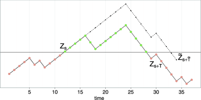
Figure 1: Trajectory of $Z$ (full line with dots) and of $\tilde{Z}$ (dotted line), when these processes go above some level $\bar{Z}^{\mathrm{hi}}$ indicated by a horizontal full line. $Z$ goes above the level at time $s$, and returns below it at time $s+T$, whereas $\tilde{Z}$ stays above the level until time $s+\tilde{T}$, with $T\leq\tilde{T}$.

First let us use Lemma 3. We can take $\epsilon<1/2$ and $\eta<\min(1/2,\epsilon b/a)$. The lemma gives the existence of an integer $K$ such that if $Z_{t}\geq K$, we have the following two inequalities:

$$P[U_{t+1}=-b|U_{t}=+a,Z_{t}] > \epsilon,$$ (4)

$$P[U_{t+1}=-b|U_{t}=-b,Z_{t}] > 1-\eta.$$ (5)

Suppose that there is some time $s$ such that $Z_{s-1}\leq K$ and $Z_{s}\geq K$. Note that necessarily $Z_{s}\in[K,K+a]$. Then we define $\tilde{Z}_{s}=Z_{s}$, a new process starting at time $s$. Let $s+T$ be the first time after $s$ such that $Z_{s+T}\leq K$. We wish to show that $E[T]<\infty$.

We define the sequence of random variables $(Z_{t})_{t\geq s}$ defined by $\tilde{Z}_{s}=Z_{s}$ and $\tilde{Z}_{t+1}=\tilde{Z}_{t}+\tilde{U}_{t}$ for $t>s$, where $(\tilde{U}_{t})_{t\geq s}$ is a sequence of random variables taking the values $+a$ or $-b$.

For $s\leq t<T$, $\tilde{U}_{t}$ is defined as follows:

• if $U_{t+1}=+a$, then $\tilde{U}_{t+1}=+a$;

• if $U_{t+1}=-b$, $U_{t}=-b$ and $\tilde{U}_{t}=-b$, then $\tilde{U}_{t+1}=-b$ with probability $p_{1}=(1-\eta)/P[U_{t+1}=-b|U_{t}=-b,Z_{t}]$ and $\tilde{U}_{t+1}=+a$ otherwise;

• if $U_{t+1}=-b$, $U_{t}=+a$ and $\tilde{U}_{t}=+a$, then $\tilde{U}_{t+1}=-b$ with probability $p_{2}=\epsilon/P[U_{t+1}=-b|U_{t}=+a,Z_{t}]$ and $\tilde{U}_{t+1}=+a$ otherwise;

• if $U_{t+1}=-b$, $U_{t}=-b$ and $\tilde{U}_{t}=+a$, then $\tilde{U}_{t+1}=-b$ with probability $p_{3}=\epsilon(1+P[U_{t+1}=+a|U_{t}=-b,Z_{t}]/P[U_{t+1}=-b|U_{t}=-b,Z_{t}])$ and $\tilde{U}_{t+1}=+a$ otherwise.

For times $t\geq T$, $\tilde{U}_{t}$ is a Markov chain independent of $U_{t}$ and $Z_{t}$, with transition matrix

$$\pmatrix{1-\epsilon&\epsilon\vspace*{2pt}\cr\eta&1-\eta},$$

where the first state corresponds to $+a$ and the second state to $-b$.

First, let us check that all these probabilities are indeed less than 1. For $p_{1}$, it follows from inequality (5). For $p_{2}$, it follows from inequality (4). For $p_{3}$, we have

$$\epsilon\biggl{(}1+\frac{P[U_{t+1}=+a|U_{t}=-b,Z_{t}]}{P[U_{t+1}=-b|U_{t}=-b,Z_{t}]}\biggr{)}\leq\epsilon\biggl{(}1+\frac{\eta}{1-\eta}\biggr{)}\leq 2\epsilon\leq 1,$$

where we used the conditions $\eta<1/2$ and $\epsilon<1/2$. Hence $(\tilde{U}_{t})$ is well defined.

Lemma 5

$(\tilde{U}_{t})$ is a Markov chain over the space $\{+a,-b\}$ with transition matrix

$$\pmatrix{1-\epsilon&\epsilon\vspace*{2pt}\cr\eta&1-\eta},$$

where the first state corresponds to $\{+a\}$ and the second state to {$-b\}$.

We only need to check this for times $t\leq T$. The events $\{\tilde{U}_{t}=-b\}$ and $\{\tilde{U}_{t}=-b,U_{t}=-b\}$ are identical, hence

$$P[\tilde{U}_{t+1}=-b|\tilde{U}_{t}=-b,Z_{t}] = P[\tilde{U}_{t+1}=-b|\tilde{U}_{t}=-b,U_{t}=-b,Z_{t}]$$

$$= P[\tilde{U}_{t+1}=-b|U_{t+1}=-b,\tilde{U}_{t}=-b,U_{t}=-b,Z_{t}]$$

$${}\times P[U_{t+1}=-b|\tilde{U}_{t}=-b,U_{t}=-b,Z_{t}]$$

$$= \frac{(1-\eta)P[U_{t+1}=-b|U_{t}=-b,Z_{t}]}{P[U_{t+1}=-b|U_{t}=-b,Z_{t}]}$$

$$= 1-\eta.$$

Note that this does not depend on $Z_{t}$.

Similarly,

$$P[\tilde{U}_{t+1}=-b|\tilde{U}_{t}=+a,U_{t}=+a,Z_{t}]$$

$$\qquad=P[\tilde{U}_{t+1}=-b|U_{t+1}=-b,\tilde{U}_{t}=+a,U_{t}=+a,Z_{t}]$$

$$\qquad\quad{}\times P[U_{t+1}=-b|\tilde{U}_{t}=+a,U_{t}=+a,Z_{t}]$$

$$\qquad=\frac{\epsilon P[U_{t+1}=-b|U_{t}=+a,Z_{t}]}{P[U_{t+1}=-b|U_{t}=+a,Z_{t}]}$$

$$\qquad=\epsilon$$

and

$$P[\tilde{U}_{t+1}=-b|\tilde{U}_{t}=+a,U_{t}=-b,Z_{t}]$$

$$\qquad=P[\tilde{U}_{t+1}=-b|U_{t+1}=-b,\tilde{U}_{t}=+a,U_{t}=-b,Z_{t}]$$

$$\qquad\quad{}\times P[U_{t+1}=-b|\tilde{U}_{t}=+a,U_{t}=-b,Z_{t}]$$

$$\qquad=\epsilon\biggl{(}1+\frac{P[U_{t+1}=+a|U_{t}=-b,Z_{t}]}{P[U_{t+1}=-b|U_{t}=-b,Z_{t}]}\biggr{)}$$

$$\qquad\quad{}\times P[U_{t+1}=-b|U_{t}=-b,Z_{t}]$$

$$\qquad=\epsilon\bigl{(}P[U_{t+1}=-b|U_{t}=-b,Z_{t}]+P[U_{t+1}=+a|U_{t}=-b,Z_{t}]\bigr{)}$$

$$\qquad=\epsilon.$$

These last two calculations result in

$$P[\tilde{U}_{t+1}=-b|\tilde{U}_{t}=+a]=\epsilon$$

with no dependence on $Z_{t}$ (or $U_{t}$).

The previous lemma is central to the proof, and especially the lack of dependence on $Z_{t}$. We always have $\tilde{U}_{s}=+a$, since $U_{s}=+a$. Hence for each $t\geq s$, the distribution of $\tilde{U}_{t}$ depends only on $\eta$ and $\epsilon$, and implicitly on the threshold $K$, but not on the value of $Z_{s}$. Hence $(\tilde{U}_{t})$ has the same law, every time the process $(Z_{t})$ goes above $K$.

3.3 Conclusion: Proof of Theorem 1 and Corollary 2

Let us now use the bounding process $(\tilde{Z}_{t})$ to control the time spent by $(Z_{t})$ above $K$.

Lemma 6

There exists $\tau\in\mathbb{R}$ such that, for all times $s$ such that $Z_{s-1}\leq K$ and $Z_{s}\geq K$, and defining $T$ by $T=\inf_{d\geq 0}\{Z_{s+d}\leq K\}$, then

$$\mathbb{E}[T]\leq\tau.$$

The Markov chain $(\tilde{U}_{t})$ admits the following stationary distribution:

$$\pi_{\tilde{U}}=\biggl{(}\frac{\eta}{\epsilon+\eta},\frac{\epsilon}{\epsilon+\eta}\biggr{)}.$$

Let us denote by $\tilde{T}$ the time spent by $(\tilde{Z}_{t})$ over $K$, that is,

$$\tilde{T}=\inf_{d\geq 0}\Biggl{\{}\sum_{t=s+1}^{s+d}\tilde{U}_{t}\leq-a\Biggr{\}}.$$

Remember that $\tilde{Z}_{s}=Z_{s}\in[K,K+a]$, hence $\tilde{Z}_{s+\tilde{T}}\leq K$ (whatever the value of $Z_{s}$). Now, our choice of $\eta$ results in $a\eta<b\epsilon$ which implies $E[\tilde{T}]<\infty$ [Norris (1998)]. Let $\tau=E[\tilde{T}]$. Note that since the law of $(\tilde{U}_{t})$ does not depend on the value of $Z_{s}$, $\tau$ does not depend on $Z_{s}$.

Since, for $t\leq T$, we impose that “if $U_{t+1}=+a$, then $\tilde{U}_{t+1}=+a$,” it follows that $\forall t\leq T,U_{t}\leq\tilde{U}_{t}$. Consequently $\forall t\leq T,Z_{t}\leq\tilde{Z}_{t}$ and hence $T\leq\tilde{T}$. Note that (the distribution of) $T$ depends on the exact value of $Z_{s}$, but that $\tilde{T}$ as we have defined it has a fixed distribution. We have $E[T]\leq\tau$ (whatever the value $Z_{s}$).

Proof of Theorem 1 Let us define the following sequence of indices:

$$S_{1} = \inf_{s\geq 0}\{Z_{s-1}\leq K\mbox{ and }Z_{s}\geq K\};$$

$$S_{k} = \inf_{s\geq S_{k-1}}\{Z_{s-1}\leq K\mbox{ and }Z_{s}\geq K\}.$$

The sequence $(S_{k})$ represents the times at which the process $(Z_{t})$ goes above $K$. Moreover let us introduce the sequence of time spent above $K$,

$$T_{k}=\inf_{s\geq 0}\{Z_{S_{k}+s-1}\geq K\mbox{ and }Z_{S_{k}+s}\leq K\}.$$

We have $Z_{S_{k}}\in[K,K+a]$. Define $k(t)$ such that $S_{k(t)}\leq t<S_{k(t)+1}$. Either $Z_{t}\leq K$ or $Z_{t}>K$. In the latter case, $Z_{t}\leq Z_{S_{k(t)}}+aT_{k(t)}$. Clearly, in any case,

$$\mathbb{E}[Z_{t}]\leq(K+a)+a\tau.$$ (6)

A similar reasoning on the lower bound leads to $K^{\prime}$ and $\tau^{\prime}<\infty$ such that

$$\mathbb{E}[Z_{t}]\geq\bigl{(}K^{\prime}-b\bigr{)}-b\tau^{\prime}.$$ (7)

Inequalities (7) and (6) imply

$$\mathbb{E}\biggl{[}\frac{Z_{t}}{t}\biggr{]}\to 0.$$

As stated at the beginning of the section, for update (1) the convergence $Z_{t}/t\to 0$ (in mean) implies the convergence of the proportions $(\nu_{t}/t)$ to $\phi$ (also in mean). We now show that this ensures that the flat histogram is reached in finite time. Proof of Corollary 2 For a fixed threshold $c$, recall that FH being reached at time $t$ corresponds to the event

$$\mathrm{FH}_{t}=\biggl{\{}\forall i\in\{1,\ldots,d\}\ \biggl{|}\frac{\nu_{t}(i)}{t}-\phi_{i}\biggr{|}<c\biggr{\}}.$$

We will only use the convergence in probability of the proportions to $\phi$ for all $i$

$$\frac{\nu_{t}(i)}{t}\mathop{\longrightarrow}^{\mathbb{P}}_{t\to\infty}\phi_{i},$$

which implies

$$\forall\varepsilon>0\ \exists N\in\mathbb{N}\ \forall t\geq N\qquad\mathbb{P}(\mathrm{FH}_{t})\geq 1-\varepsilon.$$

We can hence define a stopping time $T^{\mathrm{FH}}$ corresponding to the first FH being reached,

$$T^{\mathrm{FH}}=\inf_{t\geq 0}\{\mathrm{FH}_{t}\}$$

and some $\varepsilon>0$ such that

$$\exists N\in\mathbb{N}\ \forall n\geq N\qquad\mathbb{P}\bigl{(}T^{\mathrm{FH}}\leq N+n\bigr{)}\geq\varepsilon.$$

Using Lemma 10.11 of Williams (1991), the expectation of $T^{\mathrm{FH}}$ is then finite.

4 Proof when $d\geq 2$

In this section we extend the proof to the more general case $d\geq 2$. Having proved that for $d=2$, only update (1) is valid, we now focus on this update and omit update (2).

We consider the log penalties defined for update (1) by

$$\log\theta_{t}(i)=\nu_{t}(i)(1-\phi_{i})-\bigl{(}t-\nu_{t}(i)\bigr{)}\phi_{i}=\nu_{t}(i)-t\phi_{i},$$

where $\nu_{t}(i)$ is the number of visits of $(X_{t})$ in $\mathcal{X}_{i}$. We assume without loss of generality that $\log\theta_{0}=0$. Then $(X_{t},\log\theta_{t})$ is a Markov chain, by definition of the WL algorithm. We first prove that $(X_{t},\log\theta_{t})$ is $\lambda$-irreducible, for a sigma-finite measure $\lambda$. We will require the following additional assumption on the desired frequencies $\phi$.

Assumption 5.

The desired frequencies are rational numbers,

$$\phi=(\phi_{1},\ldots,\phi_{d})\in\mathbb{Q}^{d}.$$

Lemma 7

Let $\Theta$ be the following subset of $\mathbb{R}^{d}$:

$$\Theta=\Biggl{\{}z\in\mathbb{R}^{d}\dvtx\exists(n_{1},\ldots,n_{d})\in\mathbb{N}^{d}z_{i}=n_{i}-\phi_{i}S_{n}\mbox{ where }S_{n}=\sum_{j=1}^{d}n_{j}\Biggr{\}}.$$

Then denoting by $\lambda$ the product of the Lebesgue measure $\mu$ on $\mathcal{X}$ and of the counting measure on $\Theta$, $(X_{t},\log\theta_{t})$ is $\lambda$-irreducible.

The proof essentially comes from Bézout’s lemma, and is detailed in the Appendix. Note, however, that it relies on Assumption 5, that was not required for the case $d=2$. Although not a very satisfying assumption, which is likely not to be necessary for proving the occurrence of FH in finite time, it seems to be necessary for the irreducibility of $(X_{t},\log\theta_{t})$, at least with respect to a standard sigma-finite measure. In any case, this assumption is not restrictive in practice.

Since this chain is $\lambda$-irreducible, the proportion of visits to any $\lambda$-measurable set of $\mathcal{X}\times\Theta$ converges to a limit in $[0,1]$. This implies that the vector $(\nu_{t}(i)/t)$ converges to some vector $(p_{i})$. The following is a reductio ad absurdum.

Suppose that for some $i\in\{1,\ldots,d\}$, $p_{i}\neq\phi_{i}$. Since the vectors $p$ and $\phi$ both sum to $1$, this means that for some $i$, $p_{i}<\phi_{i}$: such a state $i$ is visited less than the desired frequency.

Let $\{i_{1},i_{2},\ldots\}=\operatorname{argmin}_{1\leq j\leq d}(p_{j}-\phi_{j})$. Then for any $i_{k}$ and for $j\notin\{i_{1},\break i_{2},\ldots\}$, we have

$$Z_{t}^{j,i_{k}}=-\nu_{t}(i_{k})+\nu_{t}(j)+t(\phi_{i_{k}}-\phi_{j})\sim t(-p_{i_{k}}+\phi_{i_{k}}+p_{j}-\phi_{j})\to\infty.$$

This implies

$$\forall K>0\ \exists T\in\mathbb{N}\ \forall t>T\qquad Z_{t}^{j,i_{k}}>K.$$

Now consider the stochastic process $(U_{t})$ such that:

• $U_{t}=-b$ if $J(X_{t})\in\{i_{1},i_{2},\ldots\}$;

• $U_{t}=+a$ otherwise,

for some real numbers $a$ and $b$. Recall that the function $J$ is such that if $X_{t}\in\mathcal{X}_{i}$, then $J(X_{t})=i$.

Let $\epsilon$ be such that when $X_{t}\notin\mathcal{X}_{i_{1}}\cup\mathcal{X}_{i_{2}}\cup\cdots$, there is probability at least $\epsilon$ of proposing in $\mathcal{X}_{i_{1}}\cup\mathcal{X}_{i_{2}}\cup\cdots$. For large enough $K$, these proposals will always be accepted. As before, for large enough $K$, we can make the probability $\eta$ of leaving $\mathcal{X}_{i_{1}}\cup\mathcal{X}_{i_{2}}\cup\cdots$ as small as we wish.

Using the exact same reasoning as in Section 3, we can construct a process $(\tilde{U}_{t})$ which is a Markov chain with transition matrix

$$\pmatrix{1-\epsilon&\epsilon\vspace*{2pt}\cr\eta&1-\eta}$$

and with $U_{t}<\tilde{U}_{t}$ almost surely. Therefore for $t>T$, $(U_{t})$ decreases on average, hence $(Z_{t}^{j,i_{k}})$ decreases on average, which contradicts the assumption that it goes to infinity. Hence for all $i$, $p_{i}=\phi_{i}$.

5 Illustration of Theorem 1 on a toy example

Let us show the consequences of Theorem 1 on a simple example. We consider as the target distribution the standard normal distribution truncated to the set $\mathcal{X}=[-10,10]$. We use a Gaussian random walk proposal, with unit standard deviation. Finally we arbitrarily split the state space in $\mathcal{X}_{1}=[-10,0]$ and $\mathcal{X}_{2}=]0,10]$, and we set the desired frequencies to be $\phi=(0.75,0.25)$. Figure 2 shows the results of the Wang–Landau algorithm. Using update (1) and 200,000 iterations, we obtain the histogram of Figure 2(a). Figure 2(b) shows the convergence of the proportions of visits to each bin, using update (1). The dotted horizontal lines indicate $\phi$, and we can check that the observed proportions of visits converge toward it.

Figure 2(c) shows a similar plot, this time using update (2). Again, the desired frequencies are represented by dotted lines. Using the left-hand side of equation (3), we can calculate the theoretical limit of the observed proportion of visits in each bin, which for $\gamma=1$ and $\phi=(0.75,0.25)$, is approximately equal to $(0.79,0.21)$. Hence for a precision threshold $c$ equal to, for example, $1\%$, the occurrence of FH is not likely to occur if one uses update (2).

As expected, update (1) leads to convergence to the desired frequencies, but update (2) does not.

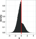
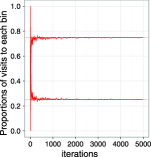
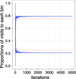
(a) Histogram of the	(b) Convergence of the	(c) Convergence of the
generated sample	proportions of visits to each bin,	proportions of visits to each bin
	using the right update	using the wrong update

Figure 2: Results of the Wang–Landau algorithm using two different updates of the penalties. Histogram of the generated sample using update (1), with a vertical line showing the binning (left). Convergence of the proportions of visits to each bin, using update (1) (middle) and using update (2) (right). The dotted horizontal lines represent the desired frequencies.

6 Discussion

As seen in Theorem 1 and Corollary 2 of Section 3, update (1) is valid, in the sense that the frequencies of visits of the chain $(X_{t})$ converges toward $\phi$. Consequently FH is met in finite time, for any threshold $c>0$.

Regarding the proof of Theorem 1 in the case $d>2$, we assume that the desired frequencies $\phi$ are rationals (Assumption 5), which allows to prove that the Markov chain generated by the algorithm $(X_{t},Z_{t})$ is $\lambda$-irreducible for some sigma-finite measure $\lambda$. However, our proof requires mainly that the proportions of visits of $(X_{t})$ to any bin $\mathcal{X}_{i}$ converge, which is equivalent to the convergence of $(Z_{t}/t)$. We believe that results on random walks in random environments [Zeitouni (2006)] would allow us to remove the rationality assumption.

Assumptions 2–4 could be relaxed by using the well-known properties of the Metropolis–Hastings algorithm, from which we did not take advantage here. More precisely, note that the Wang–Landau transition kernel differs from the Metropolis–Hastings only when the proposed points, generated through $Q(\cdot,\cdot)$, land in a different bin than the current position of the chain. Otherwise, the kernel behaves like a Metropolis–Hastings targeting $\pi$. Hence under some weaker assumptions than the one we have formulated here, it has recurrence properties.

To conclude, we have shown that for fixed $\gamma$, the Flat Histogram criterion is reached in finite time for certain updates. For other updates, the observed frequencies do not converge to the desired frequencies, and so there is a nonzero probability that the flat histogram criterion will never be verified. Note that we do not make any claims about the distribution of the sample inside each of the bins $\mathcal{X}_{i}$ at fixed $\gamma$.

Appendix: Proof of Lemma 7

Let $\Theta\subset\mathbb{R}^{d}$ be the set of possibly reachable values of the process $(\log\theta_{t})$. We define it by

$$\Theta=\Biggl{\{}z\in\mathbb{R}^{d}\dvtx\exists(n_{1},\ldots,n_{d})\in\mathbb{N}^{d}z_{i}=n_{i}-\phi_{i}S_{n}\mbox{ where }S_{n}=\sum_{j=1}^{d}n_{j}\Biggr{\}}.$$

We want to prove the existence of a measure $\lambda$ on $\mathcal{X}\times\Theta$ such that the Markov chain $(X_{t},\log\theta_{t})$ is $\lambda$-irreducible. Denote by $\mu$ the Lebesgue measure on $\mathcal{X}$, and let $A\in\mathcal{B}(\mathcal{X})$ such that $\mu(A)>0$, and let $z^{\star}\in\Theta$. Let us show that for any time $s$ at which $X_{s}=x_{s}\in\mathcal{X}$ and $\log\theta_{s}=z_{s}\in\Theta$, there exists $t>0$ such that $X_{s+t}\in A$ and $\log\theta_{s+t}=z^{\star}$ with strictly positive probability. This will prove the $\lambda$-irreducibility of $(X_{t},\log\theta_{t})$ where $\lambda$ is the product of the Lebesgue measure $\mu$ on $\mathcal{X}$ and the counting measure on $\Theta$.

Note first that for any $n=(n_{1},\ldots,n_{d})\in\mathbb{N}^{d}$, the process $(X_{t})$ can visit exactly $n_{i}$ times each set $\mathcal{X}_{i}$ (for all $i$) between some time $s+1$ and some time $s+\sum_{i=1}^{d}n_{i}$, since there is always a nonzero probability of $X_{t+1}$ visiting any $\mathcal{X}_{i}$ given $X_{t}$ and $\log\theta_{t}$ (using Assumptions 3 on the proposal distribution and the form of the MH kernel). More formally, given any $n\in\mathbb{N}^{d}$ and any time $s$, denoting $S_{n}=\sum_{i=1}^{d}n_{i}$,

$$\mathbb{P}\Biggl{(}\forall i\in\{1,\ldots,d\}\sum_{t=s+1}^{s+S_{n}}\mathbh{1}_{\mathcal{X}_{i}}(X_{t})=n_{i}\bigg{|}X_{s},\log\theta_{s}\Biggr{)}>0.$$ (8)

Furthermore since $\mu(A)>0$ and since $(\mathcal{X}_{i})_{i=1}^{d}$ is a partition of $\mathcal{X}$ (satisfying Assumption 1 on nonempty bins), there exists $B\subset A$ such that $B\subset\mathcal{X}_{i^{\star}}$ for some $i^{\star}\in\{1,\ldots,d\}$ and $\mu(B)>0$. We are going to prove the following statement, which means that there is a “path” between any pair of points in $\Theta$:

Lemma 8

$$\forall z^{1},z^{2}\in\Theta\ \exists n\in\mathbb{N}^{d}\ \forall i\in\{1,\ldots,d\}\qquad z_{i}^{1}+n_{i}-\Biggl{(}\sum_{j=1}^{d}n_{j}\Biggr{)}\phi_{i}=z_{i}^{2}.$$

Then we will conclude as follows: the Markov chain can go from any $(x_{s},z_{s})$ to some $(x_{s+t-1},z_{s+t-1})$ where $z_{s+t-1}$ can be anywhere in $\Theta$, and then in one final step to $(x_{s+t},z_{s+t})$ such that $x_{s+t}\in B$ and $z_{s+t}=z^{\star}$, since $z_{s+t-1}$ can be chosen such that $z_{s+t}=z^{\star}$ when $x_{s+t}\in B\subset\mathcal{X}_{i^{\star}}$.

The structure of the proof is the following: we prove that $(\log\theta_{t})$ can go from $0$ to $0$, then from any $z\in\Theta$ to $0$, and the possibility of going from $0$ to any $z\in\Theta$ comes from the definition of $\Theta$.

Suppose that $\log\theta_{0}=(0,\ldots,0)$, and let us prove that the process $(\log\theta_{t})$ can go back to $0$, that is, let us find a vector $n=(n_{1},\ldots,n_{2})\in\mathbb{N}^{d}$ such that

$$\forall i\in\{1,\ldots,d\}\qquad 0=n_{i}-\phi_{i}S_{n}\qquad\mbox{where }S_{n}=\sum_{j=1}^{d}n_{j}.$$

Under the rationality assumption on $\phi$ (Assumption 5), there exists $(a_{i},\ldots,\break a_{d})\in\mathbb{N}^{d}$ and $b\in\mathbb{N}$ such that $\phi_{i}=a_{i}/b$ for all $i$. Now define $n\in\mathbb{N}^{d}$ as follows:

$$\forall i\in\{1,\ldots,d\}\qquad n_{i}=k\prod_{j=1,j\neq i}^{d}\frac{1}{a_{j}},$$

where $k\in\mathbb{N}$ is such that $n_{i}\in\mathbb{N}$ for all $i$. Then using $\sum_{j=1}^{d}\phi_{j}=1$ one can readily check that

$$\forall i\in\{1,\ldots,d\}\qquad n_{i}-\phi_{i}\Biggl{(}\sum_{j=1}^{d}n_{j}\Biggr{)}=0.$$

Hence the vector $n$ defines a possible path for $(\log\theta_{t})$ between $0$ and $0$, in $S_{n}=\sum_{j=1}^{d}n_{j}$ steps, with a strictly positive probability [using equation (8)].

A similar reasoning allows us to find a possible path from any $z\in\Theta$ to $0$. For such a $z\in\Theta$, there exists $(m_{1},\ldots,m_{d})\in\mathbb{N}^{d}$ such that

$$\forall i\in\{1,\ldots,d\}\qquad z_{i}=m_{i}-S_{m}a_{i}/b\qquad\mbox{where }S_{m}=\sum_{j=1}^{d}m_{j}.$$ (9)

We wish to show that there exits $(k_{1},\ldots,k_{d})\in\mathbb{N}^{d}$ such that $k_{i}-S_{k}a_{i}/b=-z_{i}$ for all $i$, where $S_{k}=\sum_{j=1}^{d}k_{j}$. To construct $(k_{1},\ldots,k_{d})$, we use the already introduced vector $(n_{1},\ldots,n_{d})$ such that $n_{i}-S_{n}a_{i}/b=0$ for all $i$, where $S_{n}=\sum_{j=1}^{d}n_{j}$. Putting this together with (9), we get for any $C\in\mathbb{N}$,

$$-z_{i}+C*0=-m_{i}+C*n_{i}-\frac{a_{i}}{b}(CS_{n}-S_{m}).$$ (10)

For $C$ large enough, for all $i$, $Cn_{i}-m_{i}>0$. We simply take $k_{i}=Cn_{i}-m_{i}$ for all $i$. This proves that starting from a point $z\in\Theta$ (by definition reachable from $0$), $(\log\theta_{t})$ can reach $0$ again.

References

• Andrieu, Moulines and Priouret (2005) {barticle}[mr] \bauthor\bsnmAndrieu, \bfnmChristophe\binitsC., \bauthor\bsnmMoulines, \bfnmÉric\binitsÉ. and \bauthor\bsnmPriouret, \bfnmPierre\binitsP. (\byear2005). \btitleStability of stochastic approximation under verifiable conditions. \bjournalSIAM J. Control Optim. \bvolume44 \bpages283–312.\biddoi=10.1137/S0363012902417267, issn=0363-0129, mr=2177157\bptnotecheck year\bptokimsref\endbibitem
• Andrieu and Thoms (2008) {barticle}[mr] \bauthor\bsnmAndrieu, \bfnmChristophe\binitsC. and \bauthor\bsnmThoms, \bfnmJohannes\binitsJ. (\byear2008). \btitleA tutorial on adaptive MCMC. \bjournalStat. Comput. \bvolume18 \bpages343–373. \biddoi=10.1007/s11222-008-9110-y, issn=0960-3174, mr=2461882 \bptokimsref \endbibitem
• Atchadé and Liu (2010) {barticle}[mr] \bauthor\bsnmAtchadé, \bfnmYves F.\binitsY. F. and \bauthor\bsnmLiu, \bfnmJun S.\binitsJ. S. (\byear2010). \btitleThe Wang–Landau algorithm in general state spaces: Applications and convergence analysis. \bjournalStatist. Sinica \bvolume20 \bpages209–233. \bidissn=1017-0405, mr=2640691 \bptokimsref \endbibitem
• Atchadé et al. (2009) {bincollection}[mr] \bauthor\bsnmAtchadé, \bfnmY.\binitsY., \bauthor\bsnmFort, \bfnmG.\binitsG., \bauthor\bsnmMoulines, \bfnmE.\binitsE. and \bauthor\bsnmPriouret, \bfnmP.\binitsP. (\byear2009). \btitleAdaptive Markov chain Monte Carlo: Theory and methods. In \bbooktitleBayesian Time Series Models \bpages32–51. \bpublisherCambridge Univ. Press, \baddressCambridge. \bptokimsref \endbibitem
• Bornn et al. (2011) {bmisc}[author] \bauthor\bsnmBornn, \bfnmL.\binitsL., \bauthor\bsnmJacob, \bfnmP.\binitsP., \bauthor\bsnmDel Moral, \bfnmP.\binitsP. and \bauthor\bsnmDoucet, \bfnmA.\binitsA. (\byear2011). \bhowpublishedAn adaptive interacting Wang–Landau algorithm for automatic density exploration. Available at \arxivurlarXiv:1109.3829. \bptokimsref \endbibitem
• Cunha Netto et al. (2006) {barticle}[author] \bauthor\bsnmCunha Netto, \bfnmA. G.\binitsA. G., \bauthor\bsnmSilva, \bfnmC. J.\binitsC. J., \bauthor\bsnmCaparica, \bfnmA. A.\binitsA. A. and \bauthor\bsnmDickman, \bfnmR.\binitsR. (\byear2006). \btitleWang–Landau sampling in three-dimensional polymers. \bjournalBrazilian Journal of Physics \bvolume36 \bpages619–622. \bptokimsref \endbibitem
• Fort et al. (2011) {bmisc}[author] \bauthor\bsnmFort, \bfnmG.\binitsG., \bauthor\bsnmMoulines, \bfnmE.\binitsE., \bauthor\bsnmPriouret, \bfnmP.\binitsP. and \bauthor\bsnmVandekerkhove, \bfnmP.\binitsP. (\byear2011). \bhowpublishedA central limit theorem for adaptive and interacting Markov chains. Available at \arxivurlarXiv:1107.2574. \bptokimsref \endbibitem
• Hastings (1970) {barticle}[author] \bauthor\bsnmHastings, \bfnmW. K.\binitsW. K. (\byear1970). \btitleMonte Carlo sampling methods using Markov chains and their applications. \bjournalBiometrika \bvolume57 \bpages97–109. \bptokimsref \endbibitem
• Kesten (1958) {barticle}[mr] \bauthor\bsnmKesten, \bfnmHarry\binitsH. (\byear1958). \btitleAccelerated stochastic approximation. \bjournalAnn. Math. Statist \bvolume29 \bpages41–59. \bidissn=0003-4851, mr=0093851 \bptokimsref \endbibitem
• Liang (2005) {barticle}[mr] \bauthor\bsnmLiang, \bfnmFaming\binitsF. (\byear2005). \btitleA generalized Wang–Landau algorithm for Monte Carlo computation. \bjournalJ. Amer. Statist. Assoc. \bvolume100 \bpages1311–1327. \biddoi=10.1198/016214505000000259, issn=0162-1459, mr=2236444 \bptokimsref \endbibitem
• Malakis, Kalozoumis and Tyraskis (2006) {barticle}[author] \bauthor\bsnmMalakis, \bfnmA.\binitsA., \bauthor\bsnmKalozoumis, \bfnmP.\binitsP. and \bauthor\bsnmTyraskis, \bfnmN.\binitsN. (\byear2006). \btitleMonte Carlo studies of the square Ising model with next-nearest-neighbor interactions. \bjournalEur. Phys. J. B \bvolume50 \bpages63–67. \bptokimsref \endbibitem
• Ngo and Diep (2008) {barticle}[mr] \bauthor\bsnmNgo, \bfnmV. Thanh\binitsV. T. and \bauthor\bsnmDiep, \bfnmH. T.\binitsH. T. (\byear2008). \btitlePhase transition in Heisenberg stacked triangular antiferromagnets: End of a controversy. \bjournalPhys. Rev. E (3) \bvolume78 \bpages031119, 5. \biddoi=10.1103/PhysRevE.78.031119, issn=1539-3755, mr=2496090 \bptokimsref \endbibitem
• Norris (1998) {bbook}[mr] \bauthor\bsnmNorris, \bfnmJ. R.\binitsJ. R. (\byear1998). \btitleMarkov Chains. \bseriesCambridge Series in Statistical and Probabilistic Mathematics \bvolume2. \bpublisherCambridge Univ. Press, \blocationCambridge. \bidmr=1600720 \bptokimsref \endbibitem
• Robert and Casella (2004) {bbook}[mr] \bauthor\bsnmRobert, \bfnmChristian P.\binitsC. P. and \bauthor\bsnmCasella, \bfnmGeorge\binitsG. (\byear2004). \btitleMonte Carlo Statistical Methods, \bedition2nd ed. \bpublisherSpringer, \blocationNew York. \bidmr=2080278 \bptokimsref \endbibitem
• Silva, Caparica and Plascak (2006) {barticle}[author] \bauthor\bsnmSilva, \bfnmC. J.\binitsC. J., \bauthor\bsnmCaparica, \bfnmA. A.\binitsA. A. and \bauthor\bsnmPlascak, \bfnmJ. A.\binitsJ. A. (\byear2006). \btitleWang–Landau Monte Carlo simulation of the Blume–Capel model. \bjournalPhys. Rev. E (3) \bvolume73 \bpages036702. \bptokimsref \endbibitem
• Tierney (1998) {barticle}[mr] \bauthor\bsnmTierney, \bfnmLuke\binitsL. (\byear1998). \btitleA note on Metropolis–Hastings kernels for general state spaces. \bjournalAnn. Appl. Probab. \bvolume8 \bpages1–9. \biddoi=10.1214/aoap/1027961031, issn=1050-5164, mr=1620401 \bptokimsref \endbibitem
• Wang and Landau (2001a) {barticle}[author] \bauthor\bsnmWang, \bfnmF.\binitsF. and \bauthor\bsnmLandau, \bfnmD. P.\binitsD. P. (\byear2001a). \btitleDetermining the density of states for classical statistical models: A random walk algorithm to produce a flat histogram. \bjournalPhys. Rev. E (3) \bvolume64 \bpages56101. \bptokimsref \endbibitem
• Wang and Landau (2001b) {barticle}[pbm] \bauthor\bsnmWang, \bfnmF.\binitsF. and \bauthor\bsnmLandau, \bfnmD. P.\binitsD. P. (\byear2001b). \btitleEfficient, multiple-range random walk algorithm to calculate the density of states. \bjournalPhys. Rev. Lett. \bvolume86 \bpages2050–2053. \bidissn=0031-9007, pmid=11289852 \bptokimsref \endbibitem
• Williams (1991) {bbook}[mr] \bauthor\bsnmWilliams, \bfnmDavid\binitsD. (\byear1991). \btitleProbability with Martingales. \bpublisherCambridge Univ. Press, \blocationCambridge. \bidmr=1155402 \bptokimsref \endbibitem
• Zeitouni (2006) {barticle}[mr] \bauthor\bsnmZeitouni, \bfnmOfer\binitsO. (\byear2006). \btitleRandom walks in random environments. \bjournalJ. Phys. A \bvolume39 \bpagesR433–R464. \biddoi=10.1088/0305-4470/39/40/R01, issn=0305-4470, mr=2261885 \bptokimsref \endbibitem