Abstract

The behaviour of baby universes has been an important ingredient in understanding and quantifying non-critical string theory or, equivalently, models of two-dimensional Euclidean quantum gravity coupled to matter. Within a regularized description based on dynamical triangulations, we amend an earlier conjecture by Jain and Mathur on the scaling behaviour of genus-$g$ surfaces containing particular baby universe ‘necks’, and perform a nontrivial numerical check on our improved conjecture.

PACS: 04.60.Ds, 04.60.Kz, 04.06.Nc, 04.62.+v.
Keywords: quantum gravity, lower dimensional models, lattice models.

1 Introduction

In physics, the intriguing concept of baby universes as the offspring of a parent universe – acquiring a life of their own while remaining connected to the latter – has been most concretely realized in 2d Euclidean quantum gravity models. In these models the partition function for a compact genus-$g$ surface coupled to conformal matter with central charge $c$ is given by

$$Z^{(g)}(A)=A^{\gamma(g)-3}\mbox{e}^{\mu A},$$ (1)

a formula which is exact at the conformal point (see e.g. [1]). In (1), $A$ denotes the area of the surface, $\mu$ a bare (cutoff-dependent) cosmological constant, and $\gamma(g)$ the so-called susceptibility exponent or entropy exponent, given by

$$\gamma(g)=\gamma_{0}+g(2-\gamma_{0}),~{}~{}~{}~{}\gamma_{0}=\gamma(0)=\frac{c-1-\sqrt{(c-1)(c-25)}}{12}.$$ (2)

For $c=0$, where no matter is present, the partition function (1) has an entropic interpretation, namely, it “counts” the number of surfaces of genus $g$ with area $A$. After introducing a regularization of the continuum theory, for example, by using dynamical triangulations (DT), this counting becomes literal. The continuum area is then $A=\sqrt{3}a^{2}N/4$, where $N$ is the number of triangles, and $a$ the edge length of the equilateral triangles used in DT, simultaneously acting as a UV-cutoff of the theory. The number of distinct piecewise linear surfaces (triangulations) of genus $g$ one can construct from $N$ such triangles is

$$Z^{(g)}(N)=k(g)\,N^{\gamma(g)-3}\mbox{e}^{\mu_{0}N}\left(1+{\cal O}(1/N)\right),$$ (3)

where $\mu_{0}$ is independent of the genus $g$ and $k(g)$ is a constant.

In an influential paper, Jain and Mathur (JM) related the entropy exponent $\gamma_{0}$ to the creation of baby universes [2]. They showed that the average number of so-called “minbus” (minimal neck baby universes of disc topology) of regularized area $B$ is given by

$$n_{A}(B)=k(g)\,A\left(1-B/A\right)^{\gamma(g)-2}\,B^{\gamma_{0}-2},$$ (4)

where $A$ is the regularized area of the total surface, and we assume $B<A/2$. Cutting the surface open along the minimal neck will produce two disconnected surfaces, a genus-$g$ surface of area $A\!-\!B$ with one $S^{1}$-boundary (the minimal neck), and a baby universe of area $B$, whose topology is a sphere with a single $S^{1}$-boundary (the same minimal neck), that is, a disc. In the following we will always work in a suitable DT-ensemble of triangulated surfaces and use the notation $A$ and $B$ for the number of triangles, thus ignoring the factor $a^{2}\sqrt{3}/4$ which relates the number of triangles to the area of the surface. Likewise in discrete units, the length of a minimal neck can be 1, 2 or 3 links ($\equiv$ triangle edges), depending on the choice of DT-ensemble, i.e. the regularity conditions imposed on the triangle gluings.

The leading power-law behaviour of $B$ in (4) gives us a convenient way to determine $\gamma_{0}$ in numerical simulations and has been used extensively in two dimensions, beginning with [3], as well as in higher-dimensional gravity, starting with [4].

While the derivation of (4) is robust and correct, JM put forward generalized relations, based on a certain conjectured formula involving non-minimal necks (eq. (9) in [2]), which also divide a surface into two pieces $A-B$ and $B$, but have an arbitrary length $\ell<\sqrt{A}$. The main purpose of this letter is to demonstrate that the formula conjectured in [2] is incorrect. We will discuss how to modify it appropriately, while retaining many of the results derived there. Our key observation will be that the necks of baby universes are by construction rather special curves on the two-surface, whose scaling behaviour (as function of the surface area $A$) is different from that of generic curves. We will also perform a nontrivial numerical check of our improved conjecture and suggest further applications of our new result.

2 The conjecture and how to modify it

In this section we will limit ourselves to the case $c\!=\!0$ of 2d gravity without matter, leaving the discussion of general central charge $c\leq 1$ to Sec. 4.

Consider a (triangulated) surface of area $A$ and spherical topology, except for $n$ boundary loops of length $\ell_{i}$, $i=1,\ldots,n$, counting the number of edges in the boundaries. Assume also that none of the boundary loops can be deformed into a loop of shorter length in the same homotopy class, unless the deformation sweeps an area which is a sizeable fraction of $A$. JM conjectured that the number of such surfaces behaves like

$${\tilde{Z}}_{n}(A,\ell_{i})\sim Z^{(g=0)}(A)\;A^{n}\prod_{i=1}^{n}\ell_{i}^{-(1+\gamma_{0})}.$$ (5)

The factor $A^{n}\,Z^{(g=0)}(A)$ is uncontroversial, with $A^{n}$ counting the number of ways $n$ boundary loops can be located on a surface of area $A$. In addition, JM made the general ansatz $1/\ell^{(1+\alpha)}$, where $\ell$ is less than some fraction of $\sqrt{A}$. To determine $\alpha$, they calculated the genus-one partition function from ${\tilde{Z}}_{2}(A,\ell,\ell)$ by gluing together the two boundaries to form a torus and integrating over $\ell$ up to $\sqrt{A}$,

$$Z^{(g=1)}(A)\sim\int^{\sqrt{A}}d\ell\;\ell\;{\tilde{Z}}_{2}(A,\ell,\ell),$$ (6)

where the factor $\ell$ in the integrand takes into account the number of different gluings of the two boundary loops. Comparing to (1) and (2) one obtains $\alpha=\gamma_{0}$.

A number of interesting results were derived in [2] using the ansatz (5). For example, it is straightforward to obtain the relation $\gamma(g)=\gamma_{0}+g(2-\gamma_{0})$ by employing (5) for a surface $A$ with $g$ pairs of boundaries of equal loop length $\ell_{i}$, $i=1,\ldots,g$, and thus $n=2g$. General genus-$g$ surfaces are created by gluing together the loops of each pair and integrating over the corresponding length variable $\ell_{i}$, generalizing (6). It is easy to see that each such operation will create a factor $A^{2-\gamma_{0}}$.

As pointed out in [2], the number of spherical surfaces of area $A$ with $n$ boundaries which cannot be deformed without increasing their length is strictly smaller than the number of surfaces when the $n$ boundaries are arbitrary, for which standard formulas exist. This happens because boundaries which serve as baby universe necks in the sense of JM are special curves. However, the consequences of this are even more drastic than envisaged in [2], and are directly related to why the ansatz (5) is not entirely correct. The boundary loop in (5) is by definition a geodesic curve, and it is well known that geodesics scale anomalously in the DT ensemble of surfaces [9, 10, 11, 12, 13]. In fact, the dimension of geodesic curves is volume^1/4 and not volume^1/2, as one might have expected naïvely, implying that the Hausdorff dimension $d_{h}$ of surfaces in the DT ensemble is 4. This is reflected in the scaling behaviour of the expectation values (w.r.t. the ensemble average)

$$\langle R\rangle_{A}\sim A^{1/d_{h}},~{}~{}\langle A(r)\rangle_{A}\sim r^{d_{h}},~{}~{}r\ll A^{1/d_{h}},\;\;{\rm where}\;d_{h}=4\;\;\;(c=0),$$ (7)

where $R$ is the linear extension of a surface of area $A$, and $A(r)$ the area contained within a geodesic distance $r$ from a given point.

The necks of length $\ell$ along which JM cut surfaces into disconnected pieces are geodesic curves, which means that their ensemble average is much shorter than the generic $\sqrt{A}$ used in [2] as upper limit in integrations like (5). (Note that the main contribution to this integral comes precisely from the upper limit.) Instead, according to (7), $A^{1/4}$ should be used as upper limit, and, more generally, $A^{1/d_{h}}$ if the Hausdorff dimension is $d_{h}$. An alternative ansatz, which will reproduce most of the results of [2], is to replace (5) by

$${\tilde{Z}}_{n}^{\prime}(A,\ell_{i})\sim Z^{(g=0)}(A)\;A^{n}\prod_{i=1}^{n}\ell_{i}^{-(1+\gamma_{0}d_{h}/2)}\;\;\;(c=0).$$ (8)

This formula is supposed to be valid for $\ell_{i}<A^{1/d_{h}}$, with the understanding that any integrations over $\ell_{i}$ are to be performed from the minimal neck length up to $A^{1/d_{h}}$. For $\ell_{i}>A^{1/d_{h}}$ the function ${\tilde{Z}}_{n}^{\prime}(A,\ell_{i})$ is assumed to vanish fast.

3 Testing the new ansatz

As an application of the new ansatz (8), let us reconsider the torus case, where relation (6) is now replaced by

$$Z^{(g=1)}(A)\sim\int^{A^{1/4}}d\ell\;\ell\;{\tilde{Z}}^{\prime}_{2}(A,\ell,\ell).$$ (9)

We have performed a nontrivial quantitative test of the ansatz (8) by measuring the probability distribution $P_{A}(\ell)$ of the length $\ell$ of the shortest non-contractible loop in the DT ensemble of triangulations of the torus with $A$ triangles. According to (8), the distribution should be

$$P_{A}(\ell)=\frac{\ell\;{\tilde{Z}}^{\prime}_{2}(A,\ell,\ell)}{Z^{(g=1)}(A)}\sim\frac{\ell}{A^{1/2}}F\Big{(}\frac{\ell}{A^{1/4}}\Big{)},$$ (10)

where $F(0)=1$ and $F(x)$ goes rapidly to zero when $x>1$.

In practice, to find shortest non-contractible loops we need a method to determine whether a given loop is contractible or not. By a different method, we first constructed two loops $\alpha_{1}$, $\alpha_{2}$ generating the fundamental group of the torus. Whether an arbitrary loop is contractible can then be established by measuring its intersection numbers with these two generators. It is contractible if and only if both intersection numbers vanish. The shortest non-contractible loop based at any given vertex $v$ can be found by performing a so-called breadth-first search along the edges starting at $v$. Encountering a vertex that has been visited before means that one has found a loop in the triangulation. The first such loop one meets which is non-contractible will automatically have minimal length. Since any non-contractible loop must intersect at least one of the $\alpha_{i}$, in order to find the overall shortest non-contractible loop it suffices to repeat the above procedure for all vertices contained in either of the generating loops $\alpha_{i}$.

Fig. 1 shows the superimposed measurements of the rescaled probability distribution $A^{1/4}P_{A}(\ell)/(\ell/A^{1/4})$ for various values of $\ell$ and $A$. The computer simulations were performed in the DT ensemble consisting of triangulations dual to connected $\phi^{3}$-graphs with $A$ vertices and toroidal topology, including self-energy and tadpole graphs. (To be precise, the simplest self-energy subgraphs consisting of two lines and tadpole subgraphs consisting of a single line were left out to ensure that all vertices in the triangulation have an order larger than or equal to three. This is not expected to affect the final result in any way.)

If the ansatz (8) is correct we should observe a universal function of $x=\ell/A^{1/4}$ which goes to a constant for $x\to 0$. Inspection of Fig. 1 reveals that the expected finite-size scaling is indeed satisfied with good accuracy, and we obtain a universal function $F(x)$.

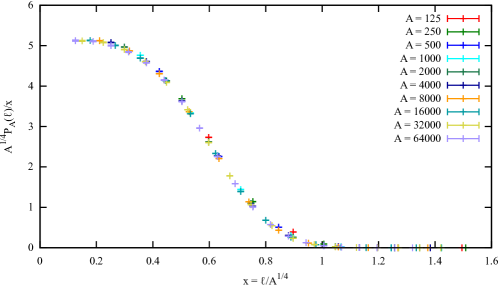
Figure 1: Plot of a rescaled version $A^{1/4}P_{A}(\ell)/(\ell/A^{1/4})$ of the probability distribution of the length of the shortest non-contractible loop on the DT ensemble of triangulated tori, as function of the rescaled length $x=\ell/A^{1/4}$, with $\ell\in[2,21]$ and areas $A$ in the range between 125 and 64000.

By contrast, the computer simulations are in clear disagreement with the ansatz of [2] which predicts a ($\ell$-independent) probability distribution

$$P_{A}^{(JM)}(\ell)\sim\frac{1}{\sqrt{A}}~{}~{}~{}{\rm for}~{}~{}~{}\ell<\sqrt{A},$$ (11)

as noted in [14]. Our improved ansatz also resolves a discrepancy found in [14], namely, that (11) leads to an average loop length $\langle\ell\rangle\sim A^{1/2}$, while one would expect $\langle\ell\rangle\sim A^{1/4}$ because of the anomalous scaling dimension of geodesic distance. It is exactly the latter relation which follows from our suggested probability distribution (10), based on the ansatz (8).

4 2d gravity coupled to conformal matter

The arguments presented above for $c\!=\!0$ need to be refined for the general case $c\!\leq\!1$, when matter is coupled to 2d gravity. The idea put forward in [2] of how to tackle this situation is to integrate out all matter degrees of freedom and work with the resulting partition function (which looks purely geometric, like the one for $c\!=\!0$), and then simply repeat the cutting-and-gluing arguments for baby universes used in the matter-free case. Although this is a well-defined procedure for a single closed surface of area $A$, and will lead to a partition function $Z^{(g)}(A)$, this is no longer true in the presence of boundaries where, to start with, boundary conditions for the matter must be specified. Examples are so-called “free boundary conditions” (where the matter configurations on the boundary are integrated over), or other specific prescriptions like Dirichlet boundary conditions for the case of a scalar field, say. No matter what choice one makes, additional weights associated with the matter on the boundary will arise, which are simply not taken into account in the treatment of [2], which crucially features “baby universe surgery” along such boundaries.

Let us illustrate this point by the case of Ising spins coupled to DT, with spins located at the centres of triangles. The Ising model has a critical point when defined on the DT ensemble, describing a $c=1/2$ conformal field theory coupled to 2d gravity [15]. If we consider a surface containing a neck and an associated baby universe, there is clearly an energy associated with the spin configurations of neighbouring triangles across the loop forming the neck, which will appear as a weight in the statistical sum over spin configurations. There is no obvious way to recover this energy contribution exactly from the separate partition functions of the two disjoint surfaces after cutting open the initial surface along the neck.

A perhaps more pertinent question is when and whether such unaccounted boundary contributions to the energy will matter. In the case of minbus the boundaries in question will have a minimal number of edges (one, two, or three, depending on the choice of DT ensemble), and any energy contribution associated with them will become negligible in the continuum limit. This explains why the relations derived by JM are robust for the case of baby universes of minimal neck size, even when $c\not=0$. As already mentioned in passing, their relation (4) for the average minbu number has been used to measure $\gamma_{0}$ also in the matter-coupled case, and agreement with the theoretical value for $\gamma_{0}$ was found.

The derivations in [2] building on the ansatz (5) for general, non-minimal necks are much harder to justify. When the boundary lengths $\ell$ become of the order of the linear system size (it is precisely those large $\ell$-values which give important contributions to integrals like (6), as noted earlier), the contributions from boundary energies become potentially significant, but are very difficult to control. Nevertheless, let us for the sake of simplicity assume that we can ignore such boundary energies when decomposing surfaces and that a suitable generalization of the ansatz (8) is valid, and see where this leads us.

For definiteness, consider the Ising model on the DT ensemble as described above. As long as the coupling constant of the Ising model stays away from its critical value, the geometric behaviour of the model will be identical to that of the pure-gravity case with $c=0$ and $d_{h}=4$, and captured by our earlier ansatz (8), together with the new insight that the linear size of the surface is not given by the ‘naïve’ $A^{1/2}$, but by $A^{1/4}$. By contrast, if we fine-tune the Ising coupling to its critical value, the interaction between geometry and spins will be such that the fractal structure of spacetime is altered, manifesting itself in a larger Hausdorff dimension $d_{h}({\it Ising})\!>\!4$. This also implies that the effective linear size of the system is decreased to $A^{1/d_{h}({\it Ising})}$. It makes it tempting to conjecture that a straightforward generalization of (8), namely,

$${\tilde{Z}}_{n}^{\prime}(A,\ell_{i})\sim Z^{(g=0)}(A)\;A^{n}\prod_{i=1}^{n}\ell_{i}^{-(1+\gamma_{0}(c)d_{h}(c)/2)}\;\;\;({\rm any}\ c\leq 1),$$ (12)

is a suitable ansatz in the matter-coupled case too. It accommodates the change in Hausdorff dimension, as well as reproducing the correct partition function $Z^{(g=1)}(A)$ for the Ising model on a torus. The general formula for $d_{h}$ as a function of the central charge $c$ of the conformal field theory to be used in (12) is [16]

$$d_{h}(c)=2\frac{\sqrt{25-c}+\sqrt{49-c}}{\sqrt{25-c}+\sqrt{1-c}},$$ (13)

together with the expression given in (2) for $\gamma_{0}(c)$. The relation which generalizes (10) is

$$P_{A}(\ell)\sim A^{-1/d_{h}(c)}\Big{(}\frac{\ell}{A^{1/d_{h}(c)}}\Big{)}^{|\gamma_{0}(c)|d_{h}(c)-1}F\Big{(}\frac{\ell}{A^{1/d_{h}(c)}}\Big{)},$$ (14)

where $F(0)\!=\!1$ and $F(x)$ falls off fast for $x\!>\!1$ (and recall that $\gamma_{0}(c)\!\leq\!0$). We conclude that $A^{1/d_{h}(c)}P_{A}(\ell)$ should be a universal function $x^{\alpha}F(x)$ of the rescaled length variable $\ell/A^{1/d_{h}(c)}$, with $\alpha=|\gamma_{0}(c)|\mbox{d}_{h}(c)-1$.

One could test the prediction (12) numerically for the Ising model, where $\alpha$ should be 0.40. A more clear-cut test may be topological 2d gravity, corresponding to $c\!=\!-2$, for which $\gamma_{0}\!=\!-1$, $d_{h}\!=\!3.56$ and thus $\alpha\!=\!2.56$. A special feature of this case is that triangulated surfaces of spherical topology can be constructed recursively with the correct weight, removing the need for Monte Carlo simulations [17]. This was employed in [18] to check (13) numerically with great precision. If one can generalize the recursive generation of triangulated surfaces to toroidal topology it may be possible to obtain a high-precision determination of $\alpha$ too.

Lastly, there exists a formula for $d_{h}(c)$ different from (13), namely

$$d_{h}(c)=-\frac{2}{\gamma_{0}(c)},$$ (15)

dating all the way back to one of the original papers of quantum Liouville theory [19]. It agrees with (13) for $c\!=\!0$, where $d_{h}\!=\!4$. However, it gives $d_{h}\!\to\!0$ for $c\!\to\!-\infty$ (where one would expect $d_{h}\!=\!2$), and $d_{h}\!\to\!\infty$ for $c\!\to\!1$. It has the interesting feature that the exponent $\alpha$ introduced above equals 1, not only for $c\!=\!0$, as we have already verified, but for all $c\!<\!1$. By now it is believed that the $d_{h}(c)$ of eq. (13) does not reflect directly any geometric properties of the fluctuating geometry, but rather critical aspects of the matter fields coupled to 2d gravity. This was made explicit in [20], where it was shown that the spin clusters of the matter fields had exactly the dimension (15) for both $c\!=\!-2$ and $c\!=\!1/2$, while measurements of the geometric $d_{h}$ clearly differed from (15). Measuring the exponent $\alpha$ for $c\!=\!-2$ and $c\!=\!1/2$ as mentioned above would give us a new method, compared to [20], to decide whether (13) or (15) represents the geometric Hausdorff dimension of 2d quantum gravity coupled to matter.

Acknowledgements. JA would like to thank the Institute of Theoretical Physics and the Department of Physics and Astronomy at Utrecht University for hospitality and financial support. TB and RL acknowledge support by the Netherlands Organisation for Scientific Research (NWO) under their VICI program.

References

- [1] J. Distler, H. Kawai, Nucl. Phys. B 321 (1989) 509-527.
- [2] S. Jain, S.D. Mathur, Phys. Lett. B 286, 239-246 (1992) [hep-th/9204017].
- [3] J. Ambjørn, S. Jain, G. Thorleifsson, Phys. Lett. B 307 (1993) 34-39 [hep-th/9303149].
- [4] J. Ambjørn, S. Jain, J. Jurkiewicz, C.F. Kristjansen, Phys. Lett. B 305 (1993) 208-213 [hep-th/9303041].
- [5] J. Ambjørn, J. Correia, C. Kristjansen, R. Loll, Phys. Lett. B 475 (2000) 24-32 [hep-th/9912267].
- [6] J. Ambjørn, R. Loll, Nucl. Phys. B 536 (1998) 407-434 [hep-th/9805108].
-
[7]
J. Ambjørn, R. Loll, Y. Watabiki, W. Westra, S. Zohren,
Phys. Lett. B 670 (2008) 224-230
[arXiv:0810.2408, hep-th],
JHEP 0805 (2008) 032
[arXiv:0802.0719, hep-th];
J. Ambjørn, R. Loll, W. Westra, S. Zohren, JHEP 0712 (2007) 017 [arXiv:0709.2784, gr-qc]. - [8] J. Ambjørn, J. Jurkiewicz, Yu.M. Makeenko, Phys. Lett. B 251 (1990) 517-524.
- [9] H. Kawai, N. Kawamoto, T. Mogami, Y. Watabiki, Phys. Lett. B 306 (1993) 19-26 [hep-th/9302133].
- [10] S.S. Gubser, I.R. Klebanov, Nucl. Phys. B 416 (1994) 827-849 [hep-th/9310098].
- [11] J. Ambjørn, Y. Watabiki, Nucl. Phys. B 445 (1995) 129-144 [hep-th/9501049].
- [12] J. Ambjørn, J. Jurkiewicz, Y. Watabiki, Nucl. Phys. B 454 (1995) 313-342 [hep-lat/9507014].
- [13] H. Aoki, H. Kawai, J. Nishimura, A. Tsuchiya, Nucl. Phys. B 474 (1996) 512-528 [hep-th/9511117].
- [14] T. Jonsson, Phys. Lett. B 425 (1998) 265-268 [hep-th/9801150].
- [15] V. A. Kazakov, Phys. Lett. A 119 (1986) 140-144.
- [16] Y. Watabiki, Prog. Theor. Phys. Suppl. 114 (1993) 1-17.
- [17] N. Kawamoto, V.A. Kazakov, Y. Saeki, Y. Watabiki, Phys. Rev. Lett. 68 (1992) 2113-2116.
- [18] J. Ambjørn, K.N. Anagnostopoulos, T. Ichihara, L. Jensen, N. Kawamoto, Y. Watabiki, K. Yotsuji, Phys. Lett. B 397 (1997) 177-184 [hep-lat/9611032]; Nucl. Phys. B 511 (1998) 673-710 [hep-lat/9706009].
- [19] J. Distler, Z. Hlousek, H. Kawai, Int. J. Mod. Phys. A 5 (1990) 1093.
- [20] J. Ambjørn, K.N. Anagnostopoulos, J. Jurkiewicz, C.F. Kristjansen, JHEP 9804 (1998) 016 [hep-th/9802020].