Modified Regge calculus as an explanation of dark energy

Abstract

Using Regge calculus, we construct a Regge differential equation for the time evolution of the scale factor $a(t)$ in the Einstein-de Sitter cosmology model (EdS). We propose two modifications to the Regge calculus approach: 1) we allow the graphical links on spatial hypersurfaces to be large, as in direct particle interaction when the interacting particles reside in different galaxies, and 2) we assume luminosity distance $D_{L}$ is related to graphical proper distance $D_{p}$ by the equation $D_{L}=(1+z)\sqrt{\overrightarrow{D_{p}}\cdot\overrightarrow{D_{p}}}$, where the inner product can differ from its usual trivial form. The modified Regge calculus model (MORC), EdS and $\Lambda$CDM are compared using the data from the Union2 Compilation, i.e., distance moduli and redshifts for type Ia supernovae. We find that a best fit line through $\displaystyle\log{\left(\frac{D_{L}}{\mbox{Gpc}}\right)}$ versus $\log{z}$ gives a correlation of 0.9955 and a sum of squares error (SSE) of 1.95. By comparison, the best fit $\Lambda$CDM gives SSE = 1.79 using $H_{o}$ = 69.2 km/s/Mpc, $\Omega_{M}$ = 0.29 and $\Omega_{\Lambda}$ = 0.71. The best fit EdS gives SSE = 2.68 using $H_{o}$ = 60.9 km/s/Mpc. The best fit MORC gives SSE = 1.77 and $H_{o}$ = 73.9 km/s/Mpc using $R=A^{-1}$ = 8.38 Gcy and $m=1.71\times 10^{52}$ kg, where $R$ is the current graphical proper distance between nodes, $A^{-1}$ is the scaling factor from our non-trival inner product, and $m$ is the nodal mass. Thus, MORC improves EdS as well as $\Lambda$CDM in accounting for distance moduli and redshifts for type Ia supernovae without having to invoke accelerated expansion, i.e., there is no dark energy and the universe is always decelerating.

Keywords :Regge calculus, dark energy, $\Lambda$CDM, Einstein-de Sitter universe

1 Introduction

The problem of cosmological “dark energy” is by now well known[1][2][3][4][5][6]. Essentially, redshifts and distance moduli for type Ia supernovae indicate the universe is in a state of accelerated expansion when analyzed using general relativistic cosmology[7][8][9]. Specifically, the distance moduli increase with increasing redshift faster than predicted by general relativistic cosmology using matter alone. Until this discovery in 1998, the so-called “standard model of cosmology” was general relativistic cosmology with a perfect fluid stress-energy tensor and an early period of inflation. Since this leads to a decelerating expansion (except during the short, early inflationary period), something ‘exotic’ seemed to be required to account for the unexpectedly large distance moduli at larger redshifts, viz., dark energy that causes the universe to change from deceleration to acceleration at about $z$ = 0.752 [9]. The new “standard model of cosmology,” i.e., that with the most robust fit to all observational data ($\Lambda$CDM), simply adds a cosmological constant $\Lambda$ to the Einstein-de Sitter cosmology model ($\Omega_{M}+\Omega_{\Lambda}=1$) and $\Lambda$ then provides the mechanism for accelerated expansion, i.e., it provides the dark energy. The “problem” is that our best theories of quantum physics tell us the cosmological constant should be exactly zero[10] or something hideously large[11], and neither of these two cases holds in $\Lambda$CDM. Thus, one of the most pressing problems in cosmology today is to account for the unexpectedly large distance moduli at larger redshifts observed for type Ia supernovae[6].

The most popular attempts to explain the apparent accelerating expansion of the universe include quintessence[11][12][13] and inhomogeneous spacetime[1][2][3][4][14] (there are even combinations of the two[15][16]). Although these solutions have their critics[17], they are certainly promising approaches. Another popular attempt is the modification of general relativity (GR). These approaches, such as f(R) gravity[18][19][20][21][22][23], have stimulated much debate[24][25][26], which is a healthy situation in science. Herein, we propose a new approach to the modification of GR via its graphical counterpart, Regge calculus.

Specifically, we construct a Regge differential equation for the time evolution of the scale factor $a(t)$ in the Einstein-de Sitter cosmology model (EdS), then we propose two modifications, both motivated by our work on foundational issues[27][28][29]. First, we allow spatial links of the Regge graph to be large (as defined below) in accord with 1) our form of direct particle interaction between sources in different galaxies and 2) the assumption that Regge calculus is fundamental while GR is the continuous approximation thereto. Of course, direct particle interaction in its original form would require a modification to general relativistic cosmology in and of itself[30][31][32][33][34][35]. We are not concerned with saving direct particle interaction in its original form and, indeed, one needn’t accept our version thereof to consider the modifications of GR proposed herein, i.e., empirical motivations suffice. Second, we do not assume that luminosity distance $D_{L}$ is trivially related to graphical proper distance $D_{p}$ between photon receiver and emitter as it is in EdS, i.e., in EdS $D_{L}=(1+z)d_{p}$ where $d_{p}$ is proper distance between photon receiver and emitter. There are two reasons we do not make this assumption. First, in our view, space, time and sources are co-constructed, yet $D_{p}$ is found without taking into account EM sources responsible for $D_{L}$. That is to say, in Regge EdS (as in EdS) we assume that pressureless dust dominates the stress-energy tensor and is exclusively responsible for the graphical notion of spatial distance $D_{p}$. However, even though the EM contribution to the stress-energy tensor is negligible, EM sources are being used to measure the spatial distance $D_{L}$. Second, in the continuous, GR view of photon exchange, one considers light rays (or wave fronts) in an expanding space to find $D_{L}=(1+z)d_{p}$. In our view, there are no “photon paths being stretched by expanding space,” so we cannot simply assume $D_{L}=(1+z)D_{p}$ as in EdS. Indeed, we find the trivial EdS relationship between luminosity distance and proper distance holds only when $D_{p}$ is small on cosmological scales. In order to generate a relationship between $D_{L}$ and $D_{p}$, we turned to the self-consistency equation $KQ=J$ in our foundational approach to physics[28], where $K$ is the differential operator, $Q$ is the ‘field’ and $J$ is the source. Since we want a relationship between $D_{L}$ and $D_{p}$, the ‘field’ of interest is a metric $h_{\alpha\beta}$ relating the graphical proper distance $D_{p}$, obtained theoretically using no EM sources, to the luminosity distance $D_{L}$, obtained observationally via EM sources. The region in question (inter-nodal region between emitter and receiver) has metric $\eta_{\alpha\beta}$ given by $ds^{2}=-c^{2}dt^{2}+dD_{p}^{2}$, so the inner product of interest can be written $\eta_{\alpha\beta}+h_{\alpha\beta}$ where the spatial coordinate is $D_{p}$ and $h_{\alpha\beta}$ is diagonal. Since each EM source proper is not “stretched out” by the expansion of space, the spatiotemporal relationship between emitter and receiver is modeled per this inter-nodal region alone. Thus, unlike EdS, we have no a priori basis in our form of direct particle interaction to relate $D_{L}$ to $D_{p}$, so we begin with the assumption $D_{L}=(1+z)\sqrt{\overrightarrow{D_{p}}\cdot\overrightarrow{D_{p}}}=(1+z)D_{p}\sqrt{1+h_{11}}$, where $\overrightarrow{D_{p}}=(0,D_{p})$.

The specific form of $KQ=J$ that we used was borrowed from linearized gravity in the harmonic gauge, i.e., $\partial^{2}h_{\alpha\beta}=-16\pi G(T_{\alpha\beta}-\frac{1}{2}\eta_{\alpha\beta}T)$. We emphasize that $h_{\alpha\beta}$ here corrects the graphical inner product $\eta_{\alpha\beta}$ in the inter-nodal region between the worldlines of photon emitter and receiver, where $\eta_{\alpha\beta}$ is obtained via a matter-only stress-energy tensor. Since the EM sources are negligible in the matter-dominated solution, we have $\partial^{2}h_{\alpha\beta}=0$ to be solved for $h_{11}$. Obviously, $h_{11}=0$ is the solution that gives the trivial relationship, but allowing $h_{11}$ to be a function of $D_{p}$ allows for the possibility that $D_{L}$ and $D_{p}$ are not trivially related. We have $h_{11}=AD_{p}+B$ where $A$ and $B$ are constants and, if the inner product is to reduce to $\eta_{\alpha\beta}$ for small $D_{p}$, we have $B=0$. Presumably, $A$ should follow from the corresponding theory of quantum gravity, so an experimental determination of its value provides a guide to quantum gravity per our view of classical gravity. As we will show, our best fit to the Union2 Compilation data gives $A^{-1}$ = 8.38 Gcy, so the correction to $\eta_{11}$ is negligible except at cosmological distances, as expected. Essentially, we’re saying the dark energy phenomenon is an indication that $A\neq 0$ so that one cannot simply assume the distance $D_{L}$ measured using EM sources corresponds trivially to the graphical proper distance $D_{p}$ even though the EM sources contribute negligibly to the stress-energy tensor.

One might also ask about distance corrections per $h_{00}$, i.e., as regards redshift, but since redshift distances are fractions of a meter one wouldn’t expect $h_{00}$ to be of consequence here. Of course, there is the issue of origin of redshift in our approach, since typically cosmological redshift is understood to occur between emission and reception[36] while clearly it must occur during emission and reception in our view. While we don’t have photons propagating through otherwise empty space between emitter and receiver, we do relate the reception and emission events in null fashion through the simplices spanning the inter-nodal region between emitter and receiver. Using the metric in each simplex $ds^{2}=-c^{2}dt^{2}+dD_{p}^{2}$, as above, we have $dD_{p}=ad\chi$, just as in EdS, although $t$ is not proper time for the nodal observers as it is in EdS. This difference in $t$ is accounted for in the computation of $D_{p}$ where it has a small effect for the range of data in the Union2 Compilation. Likewise, we do not find that it leads to a significant difference in scale factor at time of emission $a_{e}$ as a function of $z$ for the data range in question. Not surprisingly, when we compute the redshift graphically we find it is equivalent to the special relativity (SR) result, i.e., $\displaystyle z+1=\sqrt{\frac{(1+V_{e}/c)(1+V_{r}/c)}{(1-V_{e}/c)(1-V_{r}/c)}}$ where $V_{e}$ is the velocity of the emitter at time of emission in the (1+1)-dimensional inter-nodal frame and $V_{r}$ is the velocity of the receiver at time of reception. Using this form of redshift in the EdS model and comparing the result to the use of cosmological redshift in EdS, we find there is no significant difference between the two results for distance modulus $\mu$ versus redshift $z$ well beyond the range of the Union2 Compilation ($z<2$, see Figure 2). Therefore, we use cosmological redshift $\displaystyle a_{e}=\frac{1}{1+z}$ for the computation of $D_{p}$, since cosmological redshift is far simpler than the graphical alternative.

While these modifications are motivated by our work on foundational issues, their specific mathematical instantiations are herein aimed at explaining dark energy. Since this is our first foray into modified Regge calculus (MORC), the specific approaches required for explaining other GR phenomena, e.g., the perihelion shift of Mercury, remain to be seen. A defense of MORC will not be undertaken here, interested readers are referred to our earlier work cited above, but a couple comments are perhaps in order. First, the graphical lattice used herein to obtain $a(t)$ clearly violates isotropy and is not to be understood as a literal picture of the distribution of matter in the universe, e.g., galactic clusters, voids, etc. In a sense, the graphical lattice we use is no coarser an approximation than the continuum counterpart it is designed to replace, i.e., the featureless perfect fluid model of EdS where there is absolutely no structure. Rather, the graphical lattice simply provides a ‘mean’ evolution for the scale factor $a(t)$ in the equation for $D_{p}$. Second, the goal of such idealized models is to attempt to isolate ‘average’ geometric and/or material features of cosmology which broadly capture kinematic properties of the universe as a whole. Only when such models show some initial success are explorations into departures from their simplistic structure motivated, e.g., the inhomogeneous spacetime models cited above. Thus, the model we present herein was designed merely to test the possibility of replacing the continuous EdS cosmology with a discrete, graphical counterpart based on our form of direct particle interaction (again, for reasons unrelated to dark energy). Only upon some success of this initial test, i.e., improving the EdS fit to the type Ia supernova data, should we proceed to address the commensurate questions and implications of this approach (as outlined briefly in section 4 of this paper). We believe the results presented herein establish precisely “some initial success” and therefore justify further exploration into this idea.

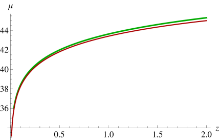
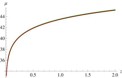
Figure 6: Top graph shows Regge evolution (red) without $h_{11}$ correction and EdS evolution (green) for case 1 Table 1 where the “stop point” $z$ is 2.05. The bottom graph makes the same comparison for case 21 Table 1 where the “stop point” $z$ is 9.98.

We begin in section 2 with an overview of Regge calculus and present our temporally continuous, spatially discrete Regge EdS equation for the time evolution of the scale factor $a(t)$ and the commensurate equation for proper distance between photon emitter and receiver $D_{p}$ in a direct inter-nodal exchange. As we will see, the spatially discrete Regge EdS equation for the time evolution of the scale factor $a(t)$ reproduces that of EdS when spatial links are small. Spatial links are “small” when the ‘Newtonian’ graphical velocity $v$ between spatially adjacent nodes on the Regge graph is small compared to c, i.e., $\displaystyle\left(\frac{v}{c}\right)^{2}\ll 1$. In that case the dynamics between adjacent spatial nodes is just Newtonian and the evolution of $a(t)$ in Regge EdS is equal to that in EdS. Deviations in the evolution of $a(t)$ between Regge EdS and MORC turn out to be small (see Figure 6). Thus, the modification of Regge evolution plays a relatively minor role in the MORC fits. Rather, as we will show, the major factor in improving EdS is $D_{L}=(1+z)D_{p}\rightarrow D_{L}=(1+z)\sqrt{\overrightarrow{D_{p}}\cdot\overrightarrow{D_{p}}}$. Since Regge EdS should give EdS when used as originally intended[37], the proposed mechanism for EM coupling in MORC differs from that in Regge calculus. When $v\approx 2c$ Regge EdS encounters the “stop point” problem[38][39][40], i.e., the backward time evolution of $a(t)$ halts, so $a(t)$ has a minimum and there is a maximum value of $z$ for which one can find $D_{p}$. Of course, this is not a real problem for Regge EdS if one is simply using it to model EdS, since one can regularly check $v$ in the computational algorithm and refine the size of the lattice to ensure $v$ remains small. However, in our case the graphical approach is fundamental, so lattice refinements are not mere mathematical adjustments, but would constitute new ‘mean’ configurations of matter. Of course, such refinements are certainly required in earlier cosmological eras, but one would expect there exists a smallest spatial scale (associated with a smallest nodal mass) so that eventually (evolving backwards in time) $v\approx 2c$ could not be avoided and the minimum $a(t)$ would be reached. Thus, there are significant deviations from our use of Regge calculus and its (originally intended) use as a graphical approximation to GR.

In section 3 we present the fits for EdS, MORC, and $\Lambda$CDM to the Union2 Compilation data, i.e., distance moduli and redshifts for type Ia supernovae[41] (see Figures 4 and 5). We find that MORC improves EdS as much as $\Lambda$CDM in accounting for distance moduli and redshifts for type Ia supernovae even though the MORC universe contains no dark energy is therefore always decelerating. While we do not need to invoke dark energy, we do propose modifications to classical gravity. Thus, it is a matter of debate as to which approach ($\Lambda$CDM or MORC) is better.

Of course, the success of MORC in this context does not commit one to our foundational motives. In fact, one may certainly dismiss our form of direct particle interaction and simply suppose that the metric established by EM sources deviates from that of pressureless dust at cosmological distances in a graphical approach to gravity. Since motives are not germane to physics, we will not present arguments for our foundational motives here. Abandoning our motives but keeping the MORC formalism would simply result in a situation similar to that in $\Lambda$CDM where a cosmological constant is added to EdS for empirical reasons. That is, one could simply view MORC as a modification of Regge calculus for empirical reasons without buying into our story about direct particle interaction and co-constructed space, time and sources. Motives notwithstanding, we believe our MORC formalism may provide creative new approaches to other long-standing problems, e.g., quantum gravity, unification, and dark matter. We conclude in section 4 by briefly outlining future directions and challenges for this research program.

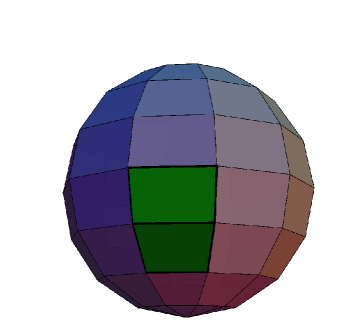
Figure 1: (a) Tessellated sphere and (b) two “flattened” trapezoids (green) from the sphere.

2 Overview of Regge Calculus

Regge calculus is typically viewed as a discrete approximation to GR where the discrete counterpart to Einstein’s equations is obtained from the least action principal on a 4D graph[37][42][43][44]. This generates a rule for constructing a discrete approximation to the spacetime manifold of GR using small, contiguous 4D Minkowskian graphical ‘tetrahedra’ called “simplices.” The smaller the legs of the simplices, the better one may approximate a differentiable manifold via a lattice spacetime (Figure 1). Although the lattice geometry is typically viewed as an approximation to the continuous spacetime manifold, it could be that discrete spacetime is fundamental while “the usual continuum theory is very likely only an approximation[45]” and that is what we assume. Curvature in Regge calculus is represented by “deficit angles” (Figure 1) about any plane orthogonal to a “hinge” (triangular side of a tetrahedron, which is a side of a simplex), so curvature is said to reside on the hinges. A hinge is two dimensions less than the lattice dimension, so in 2D a hinge is a zero-dimensional point (Figure 1). The Hilbert action for a vacuum lattice is $\displaystyle I_{R}=\frac{1}{8\pi}\displaystyle\sum_{\sigma_{i}\in L}\varepsilon_{i}A_{i}$ where $\sigma_{i}$ is a triangular hinge in the lattice L, $A_{i}$ is the area of $\sigma_{i}$ and $\varepsilon_{i}$ is the deficit angle associated with $\sigma_{i}$. The counterpart to Einstein’s equations is then obtained by demanding $\displaystyle\frac{\delta I_{R}}{\delta\ell_{j}^{2}}=0$ where $\ell_{j}^{2}$ is the squared length of the $j^{th}$ lattice edge, i.e., the metric. To obtain equations in the presence of matter-energy, one simply adds the matter-energy action $I_{M}$ to $I_{R}$ and carries out the variation as before to obtain $\displaystyle\frac{\delta I_{R}}{\delta\ell_{j}^{2}}=-\frac{\delta I_{M}}{\delta\ell_{j}^{2}}$ [46]. The LHS becomes $\displaystyle\frac{\delta I_{R}}{\delta\ell_{j}^{2}}=\frac{1}{16\pi}\displaystyle\sum_{\sigma_{i}\in L}\varepsilon_{i}\cot\Theta_{ij}$ where $\Theta_{ij}$ is the angle opposite edge $\ell_{j}$ in hinge $\sigma_{i}$. One finds the stress-energy tensor is associated with lattice edges, just as the metric, and Regge’s equations are to be satisfied for any particular choice of the two tensors on the lattice. The extent to which Regge calculus reproduces GR has been studied[47][48][49] and general methods for obtaining Regge equations have been produced[50], but these results are of no immediate concern to us because we simply seek the Regge counterpart to a specific GR equation, i.e., a Regge differential equation for the time evolution of the scale factor $a(t)$ in EdS. Whether or not we obtain said equation will be clear by virtue of its ability to track the analytic EdS solution in the proper regime, so we will not have to delve into issues associated with the ‘accuracy’ of Regge calculus in general.

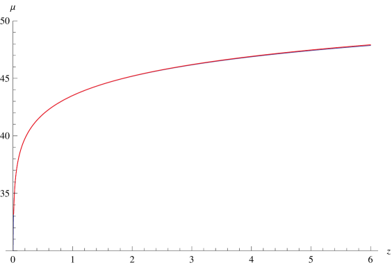
Figure 2: Comparison of cosmological redshift (blue) and graphical special relativistic redshift (red) using EdS. The two curves begin to be resolved at $z=6$.

2.1 Regge EdS Equation and MORC

Following Brewin[51] and Gentle[52], we take the stress energy associated with the worldlines of our particles to be of the form

$$\frac{12Gm}{c^{2}(ic\Delta t)}$$

so our Regge equation is

$$\frac{12iR(a_{n}+a_{n+1})}{c\Delta t}\frac{\left(\pi-\cos^{-1}\left(\frac{\left(\frac{R}{c}\right)^{2}\left(\frac{a_{n+1}-a_{n}}{\Delta t}\right)^{2}}{2\left(\left(\frac{R}{c}\right)^{2}\left(\frac{a_{n+1}-a_{n}}{\Delta t}\right)^{2}+2\right)}\right)-2\cos^{-1}\left(\frac{\sqrt{3\left(\frac{R}{c}\right)^{2}\left(\frac{a_{n+1}-a_{n}}{\Delta t}\right)^{2}+4}}{2\sqrt{\left(\frac{R}{c}\right)^{2}\left(\frac{a_{n+1}-a_{n}}{\Delta t}\right)^{2}+2}}\right)\right)}{\sqrt{\left(\frac{R}{c}\right)^{2}\left(\frac{a_{n+1}-a_{n}}{\Delta t}\right)^{2}+4}}$$

$$\hskip 252.94499pt=\frac{12iGm}{c^{3}\Delta t}$$ (1)

Multiplying both sides of (1) by $-ic\Delta t/12$ and letting $v=R(a_{n+1}-a_{n})/\Delta t$ gives

$$R(a_{n}+a_{n+1})\frac{\left(\pi-\cos^{-1}\left(\frac{v^{2}/c^{2}}{2\left(v^{2}/c^{2}+2\right)}\right)-2\cos^{-1}\left(\frac{\sqrt{3v^{2}/c^{2}+4}}{2\sqrt{v^{2}/c^{2}+2}}\right)\right)}{\sqrt{v^{2}/c^{2}+4}}=\frac{Gm}{c^{2}}$$ (2)

If $\Delta t\rightarrow 0$, then $v$ can be regarded as a ‘Newtonian’ velocity and $R(a_{n}+a_{n+1})$ can be replaced by $2r$, where $r$ is the graphical proper distance between two adjacent vertices on the lattice. Equation (2) then becomes

$$\frac{\pi-\cos^{-1}\left(\frac{v^{2}/c^{2}}{2\left(v^{2}/c^{2}+2\right)}\right)-2\cos^{-1}\left(\frac{\sqrt{3v^{2}/c^{2}+4}}{2\sqrt{v^{2}/c^{2}+2}}\right)}{\sqrt{v^{2}/c^{2}+4}}=\frac{Gm}{2rc^{2}}$$ (3)

which we emphasize is unmodified Regge calculus. If $v^{2}/c^{2}\ll 1$, then a power series expansion of the LHS of Equation (3) gives

$$\frac{v^{2}}{4c^{2}}+\mathcal{O}\left(\frac{v}{c}\right)^{4}=\frac{Gm}{2rc^{2}}$$ (4)

Thus, to leading order, our Regge EdS is EdS, i.e., $\displaystyle\frac{v^{2}}{2}=\frac{Gm}{r}$, which is just a Newtonian conservation of energy expression for a unit mass moving at escape velocity $v$ at distance $r$ from mass $m$. To better understand the relationship between Regge EdS and EdS, we note that in EdS any comoving observer A can ask, “What is the proper time rate of change of proper distance for comoving observer B at a proper distance $r$ away from me today?” The answer is precisely $v$ given by the EdS equation $\displaystyle\frac{v^{2}}{2}=\frac{Gm}{r}$, where $m$ is the mass contained inside the sphere of radius $r$ centered on observer A. In EdS the matter is distributed uniformly throughout space so the mass $m$ inside sphere of radius $r$ goes as $r^{3}$, thus $v\propto r$ on spatial hypersurfaces in the EdS equation, so there is no limit to how large $v$ is in this expression, it’s Newtonian. In Regge EdS, $v$ is the relative ‘Newtonian’ velocity of spatially adjacent nodes of mass $m$. In our view, photon exchanges occur in direct node-to-node fashion, but solving for a Regge graph between all galaxies in the universe is of course unreasonable. Instead, we use Equation (3) to provide a ‘mean’ $a(t)$ for the computation of graphical proper distance $D_{p}$ between any two photon exchangers, as in EdS, i.e.,

$$\mbox{proper distance}=\chi_{e}=c\int_{t_{e}}^{t_{o}}\frac{dt}{a}=c\int_{a_{e}}^{1}\frac{da}{a\dot{a}}$$ (5)

We then compute $D_{p}$ as a function of $z$ by using Equation (3) obtained from the ‘mean’ graph. However, before we continue there are two issues that we need to address regarding Equation (5).

First, while it is true that $cdt=ad\chi$ for a null path in a simplex and the null path will cross all values of $\chi$ between emitter and receiver, the sum of $\displaystyle d\chi=\frac{cdt}{a}$ will not equal $\chi_{e}$, i.e., the radial coordinate of the emitter. That’s because the lines of constant $\chi$ are tilted in the simplices (Figure 3), so there is a fraction of $d\chi$ (given by $\Delta$ in Figure 3) that is not accounted for by $\displaystyle\frac{cdt}{a}$. This $\Delta$ is positive on the emitter’s side of the simplex and negative on the receiver’s side, but the $\Delta$ sum on the two sides won’t cancel out exactly, since the extent of constant-$\chi$ tilt is reduced during the expansion. The correct equation for the graph is

$$\chi_{e}=c\int_{t_{e}}^{t_{o}}\left(1+\frac{2V}{c}\left(\frac{\chi(t)}{\chi_{e}}-\frac{1}{2}\right)\right)\frac{dt}{a}$$ (6)

where $V$ is the SR velocity of the emitter or receiver as a function of time and relates to our ‘Newtonian’ $v$ per

$$\frac{V}{c}=\frac{v/2c}{\sqrt{1+v^{2}/4c^{2}}}$$ (7)

To simplify the analysis and obtain an estimate of how much $\Delta$ contributes, we use EdS with $z$ = 2 and $H_{o}$ = 70 km/s/Mpc. From EdS we have $\displaystyle a(t)=\left(\frac{t}{t_{o}}\right)^{2/3}$, $\displaystyle\frac{\chi}{\chi_{e}}=1-\frac{3ct_{o}^{2/3}}{\chi_{e}}\left(t^{1/3}-t_{e}^{1/3}\right)$, and $\displaystyle\frac{v}{2c}=\frac{\chi_{e}}{3ct_{o}^{2/3}t^{1/3}}$. For $z$ = 2 and $H_{o}$ = 70 km/s/Mpc we have $t_{o}$ = 9.31 Gy, $t_{e}$ = 1.79 Gy, and $\chi_{e}$ = 11.81 Gcy. Using these values in Equation (6) we find (iteratively) $\chi_{e}$ = 12.189 Gcy. This increases $\mu$ (Equation (13) below) by 0.069 at $z$ = 2 where $\mu$ is slightly greater than 44 (Figure 5). This increase adds 0.0137 to $\displaystyle\log{\left(\frac{D_{L}}{\mbox{Gpc}}\right)}$ in our curve fitting, which amounts to a 1.3 percent increase at $z$ = 2. This change is only 0.75 percent at $z$ = 0.5 and 0.004 percent at $z$ = 0.1. Thus, given the scatter in the data, we will ignore this correction.

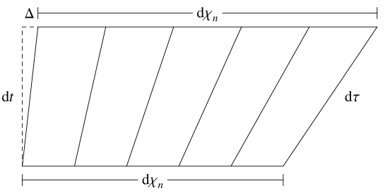
Figure 3: Lines of constant $\chi$ are tilted away from midpoint of simplex towards emitter and receiver.

Second, in EdS, the scaling factor at emission is related to the redshift by $\displaystyle a_{e}=\frac{1}{1+z}$. In EdS, this redshift is understood to occur while the radiation is in transit between emitter and receiver[36]. This “cosmological” redshift can be understood in the graphical picture to result from the fact that $dt$ in EdS runs along lines of constant $\chi$ and these lines are tilted away from the center of the simplex towards its nodal worldlines as discussed above (Figure 3). That is, $\Delta=0$ in EdS so $\displaystyle\chi_{e}=\int_{t_{e}}^{t_{o}}\frac{cdt}{a}$ holds exactly. Thus, two EdS null paths eminating from different points on a spatial link have their proper distance of separation increase from simplex to simplex. However, as explained above, our $dt$ is perpendicular to the spatial links so the null paths of successive emissions do not increase proper distance separation when traced through the simplices, i.e., redshift occurs entirely at emission and reception. Thus, relating successive events along the emitter’s worldline in null fashion to events on the receiver’s worldline, it is not surprising that we find the time delay between successive reception events as related to the temporal spacing of the emission events is that given by SR, i.e.,

$$z+1=\sqrt{\frac{(1+V_{e}/c)(1+V_{r}/c)}{(1-V_{e}/c)(1-V_{r}/c)}}$$ (8)

where $V_{e}$ is the SR velocity of the emitter at time of emission in the (1+1)-dimensional inter-nodal frame and $V_{r}$ is the SR velocity of the receiver at time of reception. Again, these SR velocities relate to our graphical ‘Newtonian’ $v$ per Equation (7). As above, we simplify the analysis using the EdS equation for $a(t)$ and find $v_{r}=\chi_{e}H_{o}$ and $\displaystyle v_{e}=\frac{\chi_{e}H_{o}}{\sqrt{a_{e}}}$ where, again, $\chi_{e}$ is the comoving coordinate of the emitter with the receiver at the origin. We need to find $\sqrt{a_{e}}$ as a function of $z$, then substitute into the equation for proper distance between photon exchangers in EdS

$$d_{p}=\frac{2c}{H_{o}}\left(1-\sqrt{a_{e}}\right)$$ (9)

Even with the simplifications, the process gets messy and ultimately was solved numerically. Since $a_{o}$ = 1, we have $d_{p}=\chi_{e}$ (as assumed in Equation 5). Let $\displaystyle x=\frac{\chi_{e}H_{o}}{2c}$ and we find

$$\sqrt{a_{e}}=x\sqrt{\frac{(A+1)^{2}}{(A-1)^{2}}-1}$$ (10)

where

$$A=\frac{(z+1)^{2}(\sqrt{1+x^{2}}-x)}{\sqrt{1+x^{2}}+x}$$ (11)

Thus, Equation (9) is $\displaystyle x=1-x\sqrt{\frac{(A+1)^{2}}{(A-1)^{2}}-1}$ and gives

$$A^{2}-2A+1-2xA^{2}+4Ax-2x+A^{2}x^{2}+x^{2}-6Ax^{2}=0$$ (12)

We then solve Equation (12) numerically for $x$ as a function of $z$ and compare with the EdS version, i.e., $\displaystyle x=1-\frac{1}{\sqrt{1+z}}$ to obtain Figure 2 where we see that there is no significant difference between the two results well beyond the range of the Union2 Compilation ($z<2$).

Since these two differences between MORC and EdS do not result in any significant difference in our fit to the data of interest, we simply use Equation (5) with $\displaystyle a_{e}=\frac{1}{1+z}$ to compute $D_{p}$. However, there is one additional difference between $d_{p}$ and $D_{p}$ when using Equation (5) that we will not ignore. We will address this additional (simple) correction in the following section where we fit EdS, MORC, and $\Lambda$CDM to the Union2 Compilation.

3 Data Analysis

The Union2 Compilation provides distance modulus $\mu$ and redshift $z$ for each supernova. In order to find $\mu$ versus $z$ for each model, we first find proper distance as a function of $z$, then compute the luminosity distance $D_{L}$, and finally

$$\mu=5\log\left(\frac{D_{L}}{10\mbox{pc}}\right)$$ (13)

For EdS we have Equation (9) for $d_{p}$, so the only parameter in fitting EdS is $H_{o}$. For $\Lambda$CDM we have $\displaystyle\dot{a}=H_{o}\sqrt{\frac{\Omega_{M}}{a}+\Omega_{\Lambda}a^{2}}$ where $\Omega_{M}+\Omega_{\Lambda}=1$. Plugging this into Equation (5) we obtain

$$d_{p}=\frac{c}{H_{o}\sqrt[4]{3}\sqrt[3]{\Omega_{m}}\sqrt[6]{\Omega_{\Lambda}}}\left[F\left(\left.\cos^{-1}\left(\frac{\sqrt[3]{\Omega_{m}}-\left(\sqrt{3}-1\right)\sqrt[3]{\Omega_{\Lambda}}}{\sqrt[3]{\Omega_{m}}+\left(\sqrt{3}+1\right)\sqrt[3]{\Omega_{\Lambda}}}\right)\right|\frac{2+\sqrt{3}}{4}\right)-\right.$$

$$\left.F\left(\left.\cos^{-1}\left(\frac{(z+1)\sqrt[3]{\Omega_{m}}-\left(\sqrt{3}-1\right)\sqrt[3]{\Omega_{\Lambda}}}{(z+1)\sqrt[3]{\Omega_{m}}+\left(\sqrt{3}+1\right)\sqrt[3]{\Omega_{\Lambda}}}\right)\right|\frac{2+\sqrt{3}}{4}\right)\right]$$ (14)

where $\displaystyle F(\phi|m)=\int_{0}^{\phi}\left(1-m\sin^{2}\theta\right)^{-1/2}d\theta$ is the elliptic integral of the first kind. Thus there are two fitting parameters for $\Lambda$CDM, $H_{o}$ and either $\Omega_{M}$ or $\Omega_{\Lambda}$. For MORC, Equation (3) gives us $a(\dot{a})$ rather than $\dot{a}(a)$, so we modify Equation (5) to read

$$D_{p}=R\int_{b_{e}}^{b_{1}}\frac{f^{\prime}(b)}{bf(b)}\sqrt{1+\frac{b^{2}}{4}}db$$ (15)

where $b=R\dot{a}/c$,

$$f(b)=\frac{\sqrt{b^{2}+4}}{2\left[\pi-\cos^{-1}\left(\frac{b^{2}}{2b^{2}+4}\right)-2\cos^{-1}\left(\frac{\sqrt{3b^{2}+4}}{2\sqrt{b^{2}+2}}\right)\right]}$$ (16)

and $b_{1}$ and $b_{e}$ respectively solve

$$1=\frac{Gm}{c^{2}R}f(b_{1})\qquad\mbox{and}\qquad a_{e}=\frac{Gm}{c^{2}R}f(b_{e})$$

The factor $\displaystyle\sqrt{1+\frac{b^{2}}{4}}$ is the correction needed to adjust the time $dt$ in Equation (5) to proper time $d\tau$ of the nodal worldlines. [This is the “one additional difference between $d_{p}$ and $D_{p}$ when using Equation (5)” alluded to at the end of section 2.] Equation (5) is then solved numerically for $D_{p}$ and $D_{L}=(1+z)D_{p}\sqrt{1+AD_{p}}$ as explained in section 1. There are three fitting parameters for MORC, the inter-nodal coordinate $R$ on the ‘mean’ graph, the nodal mass $m$ on the ‘mean’ graph, and $A^{-1}$ from $h_{11}$. Specifying $m$ and $R$ is equivalent to specifying $H_{o}$ in EdS, i.e., $\displaystyle H_{o}=\sqrt{\frac{8\pi G\rho}{3}}$ in EdS with $\rho$ given by the graphical values of $R$ and $m$ per $\displaystyle\frac{4}{3}\pi R^{3}\rho=m$. Thus compared to EdS, MORC (as with $\Lambda$CDM) has one additional fitting parameter $A^{-1}$, which presumably will be accounted for ultimately by the corresponding theory of quantum gravity.

As mentioned above, we fit these three models to the Union2 Compilation data (see Figures 4 and 5). In order to establish a statistical reference, we first found that a best fit line through $\displaystyle\log{\left(\frac{D_{L}}{\mbox{Gpc}}\right)}$ versus $\log{z}$ gives a correlation of 0.9955 and a sum of squares error (SSE) of 1.95. EdS cannot produce a better fit than this best fit line. The best fit EdS gives SSE = 2.68 using $H_{o}$ = 60.9 km/s/Mpc. A current (2011) “best estimate” for the Hubble constant is $H_{o}$ = (73.8 $\pm$ 2.4) km/s/Mpc [53]. Both MORC and $\Lambda$CDM produce better fits than the best fit line with better values for the Hubble constant than EdS. The best fit $\Lambda$CDM gives SSE = 1.79 using $H_{o}$ = 69.2 km/s/Mpc, $\Omega_{M}$ = 0.29 and $\Omega_{\Lambda}$ = 0.71. This best fit $\Lambda$CDM is consistent with its fit to the WMAP data using the latest distance measurements from BAO and a recent value of the Hubble constant[54]. The best fit MORC (case 1, Table 1) gives SSE = 1.77 and $H_{o}$ = 73.9 km/s/Mpc using $R=A^{-1}$ = 8.38 Gcy and $m=1.71\times 10^{52}$ kg. Given the scatter in the data, MORC and $\Lambda$CDM produce essentially equivalent fits, clearly superior to EdS.

The “stop point” value of $z$ in the MORC best fit is only 2.05, so we expect the Regge evolution deviates discernibly from the EdS evolution in this trial. To check this, we compared the Regge model using the best fit parameters and $h_{11}=0$ with its EdS counterpart. As explained above, the EdS counterpart to a Regge graphical result is obtained by using $\displaystyle H_{o}=\sqrt{\frac{8\pi G\rho}{3}}$ in EdS with $\rho$ given by the graphical values of $R$ and $m$ per $\displaystyle\frac{4}{3}\pi R^{3}\rho=m$. The top graph in Figure 6 shows there is in fact a discernible difference between the Regge and EdS evolutions, and the EdS value of $H_{o}$ obtained per $R$ and $m$ in this trial is 68.5 km/s/Mpc, which is significantly lower than $H_{o}$ = 73.9 km/s/Mpc found in MORC. In fact, the twenty trials with the lowest SSE values (cases 1-20, Table 1) have “stop point” $z$ less than 10, so Regge evolution, as distinct from EdS evolution, does come into play. However, Regge evolution tracks EdS evolution when “stop point” $z$ is as small 9.98 (see bottom graph in Figure 6) as is true in case 21 of Table 1. And, SSE = 1.78 for case 21 is still comparable to SSE = 1.79 of the best fit $\Lambda$CDM. The only casuality in the higher “stop point” $z$ trials is $H_{o}$, which is lowered when Regge evolution tracks EdS evolution. However, the $H_{o}$ = 71.2 km/s/Mpc in case 21 is still comparable to $H_{o}$ = 69.2 km/s/Mpc for the best fit $\Lambda$CDM. Thus, the Regge evolution plays a relatively minor role in the MORC fits. Since we used the cosmological redshift, $\displaystyle\chi_{e}=\int_{t_{e}}^{t_{o}}\frac{cdt}{a}$, and the Regge evolution played a minor role in the MORC fits, we conclude that the major factor in improving EdS is $D_{L}=(1+z)D_{p}\rightarrow D_{L}=(1+z)\sqrt{\overrightarrow{D_{p}}\cdot\overrightarrow{D_{p}}}$. Again, given the scatter of the Union2 Compilation data, we consider any of the 35 MORC results in Table 1, where SSE $\leq$ 1.78 and $H_{o}$ ranges (69.9 $\rightarrow$ 75.3) km/s/Mpc, equivalent to the best fit $\Lambda$CDM.

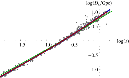
Figure 4: Plot of transformed Union2 data along with the best fits for linear regression (gray), EdS (green), $\Lambda$CDM (blue), and MORC (red).

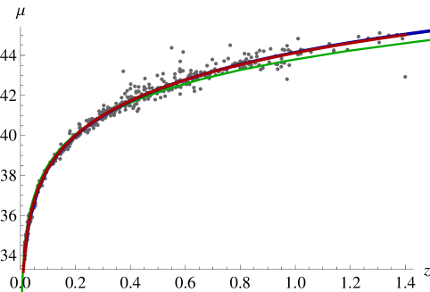
Figure 5: Plot of Union2 data along with the best fits for EdS (green), $\Lambda$CDM (blue), and MORC (red). The MORC curve is terminated at $z$ = 1.4 in this figure so that the $\Lambda$CDM curve is visible.

4 Discussion

We have explored a modified Regge calculus (MORC) approach to Einstein-de Sitter cosmology (EdS), comparing the result with $\Lambda$CDM using the Union2 Compilation of type Ia supernova data. Our motivation for MORC comes from our approach to foundational physics that involves a form of direct particle interaction whereby sources, space and time are co-constructed per a self-consistency equation. Accordingly, since EM sources are used to measure luminosity distance $D_{L}$ but are not used to compute graphical proper distance $D_{p}$, we did not expect $D_{p}$ to correspond trivially to the luminosity distance $D_{L}$, i.e., we did not assume $D_{L}=(1+z)D_{p}$. Rather, we assumed a more general relationship $D_{L}=(1+z)\sqrt{\overrightarrow{D_{p}}\cdot\overrightarrow{D_{p}}}$ where the inner product employed a correction to the inter-nodal graphical metric, $\eta_{\alpha\beta}\rightarrow\eta_{\alpha\beta}+h_{\alpha\beta}$ with spatial coordinate $D_{p}$ and $h_{\alpha\beta}$ diagonal, so that $D_{L}=(1+z)D_{p}\sqrt{1+h_{11}}$. The method used to find $h_{11}$ was a form of our self-consistency equation $KQ=J$ borrowed from the homogeneous linearized gravity equation in the harmonic gauge, i.e., $\partial^{2}h_{\alpha\beta}=0$. While $h_{11}=0$ is the solution typically used, we allowed $h_{11}$ to be a function of $D_{p}$ which gave $h_{11}=AD_{p}+B$ where $A$ and $B$ are constants. Since we wanted the inner product to reduce to $\eta_{\alpha\beta}$ for small $D_{p}$, we set $B=0$. Our best fit MORC (case 1, Table 1) gave $A^{-1}$ = 8.38 Gcy, so the correction to $\eta_{11}$ is negligible except at cosmological distances, as expected.

We found that in the context of the Union2 Compilation data MORC improved EdS as well as $\Lambda$CDM without having to employ dark energy. That is, the MORC universe evolves per pressureless dust and is always decelerating yet it accounts for distance moduli versus redshifts for type Ia supernovae as well as $\Lambda$CDM. Of course, this does not commit one to our foundational motives. In fact, one may certainly dismiss our form of direct particle interaction and simply suppose that the metric established by EM sources deviates from that of pressureless dust at cosmological distances; we did not present arguments for our foundational motives here. Abandoning our motives while keeping the MORC formalism would simply result in a situation similar to that in $\Lambda$CDM where a cosmological constant is added to EdS for empirical reasons, i.e., Regge calculus was modified to account for distance moduli versus redshifts in type Ia supernovae. Motives notwithstanding, MORC’s empirical success in dealing with dark energy gives us reason to believe this formal approach to classical gravity may provide creative new techniques for solving other long-standing problems, e.g., quantum gravity, unification, and dark matter.

In order to explore this possibility, we need to check MORC against the Schwarzschild solution, where experimental data is well established and GR is well supported. While tests of the Schwarzschild solution have been conducted on spatial scales much smaller than the cosmological scales where we found a correction to EdS, it has been shown that the simplices must be small in order to reproduce the GR redshift and the perihelion precession of Mercury in the Schwarzschild solution[55][56]. Thus, we need to verify that MORC is consistent with the Schwarzschild solution per observational data. We might refine our study of MORC cosmology, but we feel the easiest way to test MORC is via the Schwarzschild solution where perhaps the issue of dark matter can be addressed in a fashion similar to dark energy in EdS. If by chance we are able to construct a MORC for the Schwarzschild solution that passes empirical muster, we would then consider the more general issue of an action for modified Regge calculus in order to consider new approaches to quantum gravity and unification. Given the level of uncertainty involved in the next step alone, we won’t speculate further.

	$R$	$\rho$	$A^{-1}$	SSE	$H_{o}$	EdS $H_{o}$	stop point $z$
1	25.9	8.15	25.90	1.77006	73.9081	65.8705	2.04630
2	25.9	8.20	25.90	1.77092	74.1955	66.0722	2.02772
3	25.9	8.10	25.90	1.77278	73.6205	65.6681	2.06510
4	25.9	8.00	25.95	1.77453	73.0450	65.2615	2.10341
5	25.9	7.95	25.95	1.77511	72.7569	65.0572	2.12293
6	25.9	8.25	25.90	1.77532	74.4828	66.2734	2.00937
7	25.8	8.45	25.95	1.77547	72.0349	67.0719	3.65664
8	25.8	8.50	25.95	1.77638	72.2812	67.2700	3.62925
9	25.9	8.35	25.85	1.77730	75.0570	66.6738	1.97333
10	25.8	8.40	25.95	1.77742	71.7882	66.8731	3.68436
11	25.9	8.05	25.95	1.77757	73.3328	65.4651	2.08414
12	25.7	8.80	25.95	1.77821	71.6287	68.4468	6.08675
13	25.7	8.75	25.95	1.77824	71.4054	68.2521	6.12724
14	25.9	8.40	25.85	1.77852	75.3439	66.8731	1.95563
15	25.8	8.65	25.90	1.77858	73.0178	67.8610	3.54898
16	25.9	8.05	25.90	1.77914	73.3328	65.4651	2.08414
17	25.8	8.70	25.90	1.77929	73.2626	68.0568	3.52283
18	25.9	7.90	25.95	1.77938	72.4687	64.8523	2.14270
19	25.9	8.30	25.85	1.77958	74.7700	66.4739	1.99124
20	25.8	8.55	25.95	1.78009	72.5271	67.4676	3.60218
21	25.6	9.00	25.95	1.78019	71.2375	69.2203	9.98215
22	25.6	8.95	25.95	1.78053	71.0276	69.0277	10.0435
23	25.7	8.85	25.95	1.78061	71.8515	68.6410	6.04671
24	25.8	8.60	25.90	1.78065	72.7726	67.6646	3.57542
25	25.7	8.70	25.95	1.78073	71.1816	68.0568	6.16821
26	25.5	9.10	25.95	1.78171	70.8743	69.6038	16.2143
27	25.5	8.90	26.00	1.78197	70.0626	68.8347	16.6011
28	25.6	9.05	25.95	1.78206	71.4470	69.4123	9.92147
29	25.5	9.15	25.95	1.78208	71.0759	69.7947	16.1202
30	25.6	8.75	26.00	1.78209	70.1832	68.2521	10.2959
31	25.6	8.80	26.00	1.78222	70.3950	68.4468	10.2317
32	25.4	9.00	26.00	1.78226	69.9994	69.2203	26.5859
33	25.8	8.35	25.95	1.78226	71.5412	66.6738	3.71241
34	25.3	9.05	26.00	1.78236	69.9045	69.4123	42.4792
35	25.7	8.55	26.00	1.78237	70.5076	67.4676	6.29396

Table 1: Table of 35 trials that produced the best fits for MORC. Column $R$ is $X$ in $R=10^{X}\mbox{m}$. Column $\rho$ is $X$ in $\rho=X\times 10^{-27}\mbox{kg/m}^{3}$. Column $A^{-1}$ is $X$ in $A^{-1}=10^{X}\mbox{m}$. The other columns are self explanatory.

References

References

- [1] Garfinkle, D.: Inhomogeneous spacetimes as a dark energy model. Classical and Quantum Gravity 23, 4811-4818 (2006). arXiv:gr-qc/0605088v2
- [2] Paranjape, A., Singh, T.P.: The Possibility of Cosmic Acceleration via Spatial Averaging in Lemaître-Tolman-Bondi Models. Classical and Quantum Gravity 23, 6955-6969(2006). arXiv:astro-ph/0605195v3
- [3] Tanimoto, M., Nambu, Y.: Luminosity distance-redshift relation for the LTB solution near the center. Classical and Quantum Gravity 24, 3843-3857 (2007). arXiv:gr-qc/0703012
- [4] Clarkson, C., Maartens, R.: Inhomogeneity and the foundations of concordance cosmology. Classical and Quantum Gravity 27, 124008 (2010). arXiv:1005.2165v2
- [5] Perlmutter, S.: Supernovae, Dark Energy, and the Accelerating Universe. Physics Today, 53-60 (April 2003)
- [6] Bianchi, E., Rovelli, C., Kolb, R.: Is dark energy really a mystery? Nature 466, 321-322 (July 2010)
- [7] Riess, A.G., Filippenko, A.V., Challis, P., Clocchiattia, A., Diercks, A., Garnavich, P.M., Gilliland, R.L., Hogan, C.J., Jha, S., Kirshner, R.P., Leibundgut, B., Phillips, M.M., Reiss, D., Schmidt, B.P., Schommer, R.A., Smith, R.C., Spyromilio, J., Stubbs, C., Suntzeff, N.B., Tonry, J.: Observational Evidence from Supernovae for an Accelerating Universe and a Cosmological Constant. Astronomical Journal 116, 1009-1038 (1998). astro-ph/9805201
- [8] Perlmutter, S., Aldering, G., Goldhaber, G., Knop, R.A., Nugent, P., Castro, P. G., Deustua, S., Fabbro, S., Goobar, A., Groom, D. E., Hook, I. M., Kim, A. G., Kim, M. Y., Lee, J. C., Nunes, N. J., Pain, R., Pennypacker, C. R., Quimby, R., Lidman, C., Ellis, R. S., Irwin, M., McMahon, R. G., Ruiz-Lapuente, P., Walton, N., Schaefer, B., Boyle, B. J., Filippenko, A. V., Matheson, T., Fruchter, A. S., Panagia, N., Newberg, H. J. M., Couch, W. J.: Measurements of and from 42 High-Redshift Supernovae. The Astrophysical Journal 517(2) 565-586 (1999)
- [9] Suzuki, N., Rubin, D., Lidman, C., Aldering, G., Amanullah, R., Barbary, K., Barrientos, L., Botyanszki, J., Brodwin, M., Connolly, N., Dawson, K., Dey, A., Doi, M., Donahue, M., Deustua, S., Eisenhardt, P., Ellingson, E., Faccioli, L., Fadeyev, V., Fakhouri, H., Fruchter, A., Gilbank, D., Gladders, M., Goldhaber, G., Gonzalez, A., Goobar, A., Gude, A., Hattori, T., Hoekstra, H., Hsiao, E., Huang, X., Ihara, Y., Jee, M., Johnston, D., Kashikawa, N., Koester, B., Konishi, K., Kowalski, M., Linder, E., Lubin, L., Melbourne, J., Meyers, J., Morokuma, T., Munshi, F., Mullis, C., Oda, T., Panagia, N., Perlmutter, S., Postman, M., Pritchard, T., Rhodes, J., Ripoche, P., Rosati, P., Schlegel, D., Spadafora, A. Stanford, S., Stanishev, V., Stern, D., Strovink, M.,Takanashi, N., Tokita, K., Wagner, M., Wang, L., Yasuda, N., Yee, H.: The Hubble Space Telescope Cluster Supernova Survey: V. Improving the Dark Energy Constraints Above and Building an Early-Type-Hosted Supernova Sample. arXiv:1105.3470
- [10] Carroll, S.: The Cosmological Constant. arXiv:astro-ph/0004075v2 (section 4)
- [11] Weinberg, S.: The Cosmological Constant Problems. arXiv:astro-ph/0005265
- [12] Zlatev, I., Wang, L.-M., Steinhardt, P. J.: Quintessence, Cosmic Coincidence, and the Cosmological Constant. Physical Review Letters 82, 896-899 (1999)
- [13] Wang, L.M., Caldwell, R. R., Ostriker, J. P., Steinhardt, P. J.: Cosmic Concordance and Quintessence. The Astrophysical Journal 530, 17-35 (2000)
- [14] Marra, V., Notari, A.: Observational constraints on inhomogeneous cosmological models without dark energy. arXiv:1102.1015v2
- [15] Roos, M.: Quintessence-like Dark Energy in a Lemaître-Tolman-Bondi Metric. arXiv:1107.3028v2
- [16] Buchert, T., Larena, J., Alimi, J.: Correspondence between kinematical backreaction and scalar field cosmologies the ‘morphon field’. arXiv:gr-qc/0606020v2
- [17] Zibin, J.P., Moss, A., Scott, D.: Can We Avoid Dark Energy? Physical Review Letters 101, 251303 (2008)
- [18] Bernal, T., Capozziello, S., Hidalgo, J.C., Mendoza, S.: Recovering MOND from extended metric theories of gravity. arXiv:astro-ph/1108.5588v2
- [19] Nojiri, S., Odintsov, S.D.: Unified cosmic history in modified gravity: from F(R) theory to Lorentz non-invariant models. arXiv:gr-qc/1011.0544v4
- [20] Kleinert, H., Schmidt, H.J.: Cosmology with Curvature-Saturated Gravitational Lagrangian . General Relativity and Gravitation 34, 1295-1318 (2002)
- [21] Capozziello, S.: Curvature Quintessence. International Journal of Modern Physics D 11, 483 (2002). arxiv.org/pdf/gr-qc/0201033v1
- [22] Capozziello, S., Francaviglia, M.: Extended Theories of Gravity and their Cosmological and Astrophysical Applications. General Relativity and Gravitation 40, 357-420 (2008). arXiv:0706.1146v2
- [23] Olmo, G.: Palatini Approach to Modified Gravity: f(R) Theories and Beyond. International Journal of Modern Physics D 20, 413-462 (2011). arXiv:1101.3864v1
- [24] Flanagan, E.E.: The conformal frame freedom in theories of gravitation. Classical and Quantum Gravity 21, 3817 (2004)
- [25] Barausse E., Sotiriou, T.P., Miller, J.C.: A no-go theorem for polytropic spheres in Palatini f(R) gravity. Classical and Quantum Gravity 25, 062001 (2008)
- [26] Vollick, D.: On the viability of the Palatini form of 1/R gravity. Classical and Quantum Gravity 21, 3813 (2004)
- [27] Stuckey, W.M., Silberstein, M., Cifone, M.: Reconciling spacetime and the quantum: Relational Blockworld and the quantum liar paradox. Foundations of Physics 38(4), 348-383 (2008). quant-ph/0510090
- [28] Stuckey, W.M., Silberstein, M., McDevitt, T.: Relational Blockworld: A Path Integral Based Interpretation of Quantum Field Theory. quant-ph/0908.4348
- [29] Silberstein, M., Stuckey, W.M., McDevitt, T.: Being, Becoming and the Undivided Universe: A Dialogue between Relational Blockworld and the Implicate Order Concerning the Unification of Relativity and Quantum Theory (2011). quant-ph/1108.2261. Under review at Foundations of Physics.
- [30] Wheeler, J.A., Feynman, R.P.: Classical Electrodynamics in Terms of Direct Interparticle Action. Reviews of Modern Physics 21, 425 433 (1949)
- [31] Hawking, S.W.: On the Hoyle-Narlikar theory of gravitation. Proceedings of the Royal Society of London. Series A, Mathematical and Physical Sciences 286, 313 (1965)
- [32] Davies, P.C.W.: Extension of Wheeler-Feynman quantum theory to the relativistic domain I. Scattering processes. Journal of Physics A: General Physics 4, 836-845 (1971)
- [33] Davies, P.C.W.: Extension of Wheeler-Feynman quantum theory to the relativistic domain II. Emission processes. Journal of Physics A: General Physics 5, 1025-1036 (1972)
- [34] Hoyle, F., Narlikar, J.V.: Cosmology and action-at-a-distance electrodynamics. Reviews of Modern Physics 67, 113-155 (1995)
- [35] Narlikar, J.V.: Action at a Distance and Cosmology: A Historical Perspective. Annual Review of Astronomy and Astrophysics 41, 169-189 (2003)
- [36] Misner, C.W., Thorne, K.S., Wheeler, J.A.: Gravitation. W.H. Freeman, San Francisco (1973), p 772
- [37] Regge, T.: General relativity without coordinates. Nuovo Cimento 19, 558 571 (1961)
- [38] Khavari, P., Dyer, C.C.: Aspects of Causality in Parallelisable Implicit Evolution Scheme. arXiv:0809.1815v2
- [39] De Felice, A., Fabri, E.: The Friedmann universe of dust by Regge Calculus: study of its ending point. arXiv:gr-qc/0009093v1
- [40] Lewis, S.M.: Two cosmological solutions of Regge calculus. Physical Review D 25, 306 (1982)
- [41] Amanullah, R., Lidman, C., Rubin, D., Aldering, G., Astier, P., Barbary, K., Burns, M.S., Conley, A., Dawson, K.S., Deustua, S.E., Doi, M., Fabbro, S., Faccioli, L., Fakhouri, H.K., Folatelli, G., Fruchter, A.S., Furusawa, H., Garavini, G., Goldhaber, G., Goobar, A., Groom, D.E., Hook, I., Howell, D.A., Kashikawa, N., Kim, A.G., Knop, R.A., Kowalski, M., Linder, E., Meyers, J., Morokuma, T., Nobili, S., Nordin, J., Nugent, P.E., Ostman, L., Pain, R., Panagia, N., Perlmutter, S., Raux, J., Ruiz-Lapuente, P., Spadafora, A.L., Strovink, M., Suzuki, N., Wang, L., Wood-Vasey, W.M., Yasuda, N., (The Supernova Cosmology Project): Spectra and Light Curves of Six Type Ia Supernovae at and the Union2 Compilation. The Astrophysical Journal 716, 712-738 (2010). astro-ph/1004.1711v1
- [42] Misner et al (1973), p 1166
- [43] Barrett, J.W.: The geometry of classical Regge calculus. Classical and Quantum Gravity 4, 1565 1576 (1987)
- [44] Williams, R.M., Tuckey, P.A.: Regge calculus: a brief review and bibliography. Classical and Quantum Gravity 9, 1409 1422 (1992)
- [45] Feinberg, G., Friedberg, R., Lee, T.D., Ren, H.C.: Lattice Gravity Near the Continuum Limit. Nuclear Physics B245, 343-368 (1984)
- [46] Sorkin, R.: The electromagnetic field on a simplicial net. Journal of Mathematical Physics 16, 2432-2440 (1975), section II.F
- [47] Brewin, L.: Is the Regge Calculus a Consistent Approximation to General Relativity? General Relativity and Gravitation 32, 897-918 (2000)
- [48] Miller, M.A.: Regge calculus as a fourth-order method in numerical relativity. Classical and Quantum Gravity 12, 3037-3051 (1995)
- [49] Brewin, L., Gentle, A.P.: On the convergence of Regge calculus to general relativity. Classical and Quantum Gravity 18, 517-526 (2001)
- [50] Brewin, L.: Fast algorithms for computing defects and their derivatives in the Regge calculus. arXiv:1011.1885v1 (2010)
- [51] Brewin, L.: Friedmann cosmologies via the Regge calculus. Classical and Quantum Gravity 4, 899 928 (1987)
- [52] Gentle, A.P.: Regge Geometrodynamics. PhD thesis, Monash University, section 6.3 (2000)
- [53] Riess, A.G., Macri, L., Casertano, S., Lampeitl, H., Ferguson, H.C., Filippenko, A.V., Jha, S.W., Li, W., Chornock, R.: A Solution: Determination of the Hubble Constant with the Hubble Space Telescope and Wide Field Camera 3. The Astrophysical Journal 730, 119 (2011)
- [54] Komatsu, E., Smith, K.M., Dunkley, J., Bennett, C.L., Gold, B., Hinshaw, G., Jarosik, N., Larson, D., Nolta, M.R., Page, L., Spergel, D.N., Halpern, N., Hill, R.S., Kogut, A., Limon, M., Meyer, S.S., Odegard, N., Tucker, G.S., Weiland, J.L., Wollack, E., and Wright, E.L.: Seven-Year Wilkinson Microwave Anisotropy Probe (WMAP) Observations: Cosmological Interpretation. arXiv:1001.4538v3
- [55] Williams, R.M., Ellis, G.F.R.: Regge Calculus and Observations. I. Formalism and Applications to Radial Motion and Circular Orbits. General Relativity and Gravitation 13, 361-395 (1981).
- [56] Brewin, L.: Particle Paths in a Schwarzschild Spacetime via the Regge Calculus. Classical and Quantum Gravity 10, 1803-1823 (1993)