Variation of Area-to-Mass-Ratio of HAMR Space Debris Objects

Abstract

An unexpected space debris population has been detected in 2004 Schildknecht et al. , (2003, 2004) with the unique properties of a very high area-to-mass ratio (HAMR) Schildknecht et al. , (2005a). Ever since it has been tried to investigate the dynamical properties of those objects further. The orbits of those objects are heavily perturbed by the effect of direct radiation pressure. Unknown attitude motion complicates orbit prediction. The area-to-mass ratio of the objects seems to be not stable over time. Only sparse optical data is available for those objects in drift orbits.

The current work uses optical observations of five HAMR objects, observed over several years and investigates the variation of their area-to-mass ratio and orbital parameters. A normalized orbit determination setup has been established and validated with two low and two of the high ratio objects, to ensure, that comparable orbits over longer time spans are determined even with sparse optical data.

1 Introduction

The Astronomical Institute of the University of Bern (AIUB) detected high area-to-mass ratio (HAMR) objects in GEO-like orbits in 2004 Schildknecht et al. , (2003, 2004, 2005a). Since then, the AIUB observes HAMR objects on a regular basis and keeps a small catalog of HAMR and other space debris objects, which are not listed in the USSTRATCOM catalog. The observations are performed with the one meter ESA Space Debris Telescope (ESASDT), located on Tenerife, Spain, and the one meter Zimmerwald Laser and Astrometry Telescope (ZIMLAT), located in Zimmerwald, Switzerland. Additional observations for some objects, which were detected by the AIUB, are provided by courtesy of the Keldysh Institute of Applied Mathematics, Moscow, via the ISON network.

Maintaining a catalogue of HAMR objects is especially challenging due to the unique properties of these objects; the orbits are highly perturbed by direct radiation pressure. Regular observations on short time intervals are mandatory. In routine orbit determination for catalogue maintenance, variations in the value of the effective area-to-mass ratio (AMR) were detected, first investigations were performed Musci et al. , (2010).

For the investigations presented in this paper orbits are determined with an enhanced version of the CelMech tool Beutler, (2005). The area-to-mass (AMR) value is determined as a scaling parameter of the direct radiation pressure. The acceleration due to the direct radiation pressure is calculated as:

$$\vec{a}_{\text{rad}}=\frac{C}{2}\cdot\frac{S}{c}\cdot\frac{AU^{2}}{|\vec{r}-\vec{r}_{\astrosun}|^{2}}\cdot\frac{A}{m}\cdot\frac{\vec{r}-\vec{r}_{\astrosun}}{|\vec{r}-\vec{r}_{\astrosun}|},$$ (1)

where $\vec{r}$ is the geocentric position of the satellite, $\vec{r}_{\astrosun}$ the geocentric position vector of the sun, $AU$ the astronomical unit, $A$ the effective cross section exposed to the radiation, $m$ the mass of the satellite, and $c$ the speed of light. $C$ is the reflection coefficient. The direct radiation pressure is determined under the assumption of a spherically shaped object. In contrast to the calculation of the radiation pressure acceleration by other sources (compare e.g. Vallado & McCain, (2001)), the coefficient $C$ is divided by two in the formula above. A value for $C$ has to be chosen, by default, 2.0 is selected in the standard processing. This corresponds to an assumption of full absorption. All AMR values presented in this paper have to be interpreted as the effective area-to-mass ratio scaled with $C/2=1$; the AMR values of other sources may be scaled with a different factor. It is assumed that the AMR is constant over the orbital fit interval. A default value of 0.02  $\text{m}^{2}\text{kg}^{-1}$ is selected, which corresponds to an AMR value of a standard GPS satellite, in case the AMR parameter is not estimated but kept fixed in the orbit determination. For HAMR objects always an AMR value is estimated.

The shadow paths of the orbit are modeled, under the assumption of a spherical earth on a mean circular orbit; the boundary between sunlit and eclipsed part is assumed to be cylindrical, no distinction between penumbra and umbra is made, earth atmosphere is neglected.

For a long term investigation of the orbits and the AMR values, different comparable orbits have to be determined. Only sparse observations are available, which are unequally spaced in time. A normalized setup is developed, tested with two low AMR objects and two of the HAMR objects of the AIUB catalog and applied for the creation of comparable orbits for the investigation of the HAMR objects.

2 Normalized Sparse Data Setup

2.1 The Method

Four representative GEO objects from the internal catalogue of the AIUB were chosen, they have been followed over longer time periods and are not listed in the USSTRATCOM catalogue. Those objects are clearly space debris, since no maneuvers could be detected in the data. The AIUB did not have information what those objects actually were before becoming debris. From the apparent magnitude it can be concluded that those are all fragmentation pieces. They represent typical objects found in GEO surveys. Their properties are listed in Tab. 1.

Table 1: Internal name, eccentricity, inclination (deg), semi-major axis (km), area-to-mass ratio ($m^{2}/kg$) and apparent magnitude (mag) of the selected objects of the AIUB catalogue

NAME	Epoch	a	e	i	AMR	Mag
E03174A	55208.0	41900	0.001	10.1	0.01	14.6
E06321D	55275.9	41400	0.035	7.00	2.29	15.3
E06327E	54470.1	40000	0.067	12.31	0.20	17.2
E08241A	55213.0	41600	0.041	13.26	1.24	16.1

Two of the objects have low area to mass ratios, two objects qualify as HAMR objects with an AMR value larger than 1$m^{2}/kg$. The optical angle-only observations are obtained with ZIMLAT (Zimmerwald, Switzerland), and ESASDT (Tenerife, Spain), supplemented by some observations of the ISON network provided by the Keldysh Institute of Applied Mathematics, Moscow, Russia. The latter observations were obtained from different sites of the ISON network, in these particular cases, all located in Eastern Europe.

All orbits were determined from two observation sets only, using a priori orbital elements. A maximum of eight observations are allowed per set. An observation set may consist of more than one tracklet. But the observations within the sets should not be distributed over more than three days.

[ht]

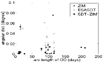
(a)

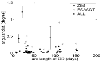
(b)

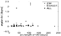
(c)

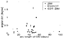
(d)

Figure 1: Angular distances as a function of the time interval between the first and the last observation of the fit interval of orbit determination for object (a) E03174A, (b) E06321D, (c) E06327E and (d) E08241A.

[h]

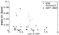
(a)

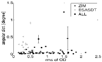
(b)

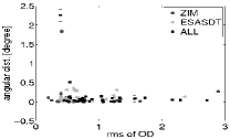
(c)

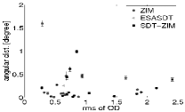
(d)

Figure 2: Root mean square of orbit determination as a function of the arc length of observations for object (a) E03174A, (b) E06321D, (c) E06327E and (d) E08241A.

[h]

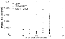
(a)

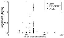
(b)

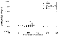
(c)

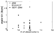
(d)

Figure 3: Angular distances as a function of the number of observations used for orbit determination for object (a) E03174A, (b) E06321D, (c) E06327E and (d) E08241A.

[h]

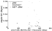
(a)

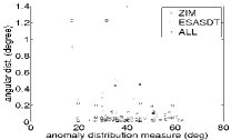
(b)

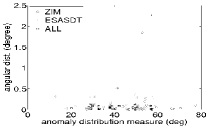
(c)

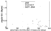
(d)

Figure 4: Angular distances as a function of anomaly distribution factor for object (a) E03174A, (b) E06321D, (c) E06327E and (d) E08241A.

[h]

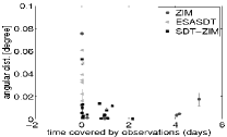
(a)

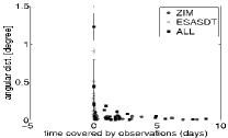
(b)

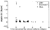
(c)

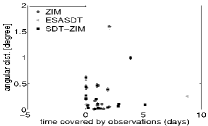
(d)

Figure 5: Angular distance as a function of time interval covered by observations used for orbit determination for object (a) E03174A, (b) E06321D, (c) E06327E and (d) E08241A.

[h]

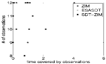
(a)

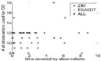
(b)

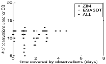
(c)

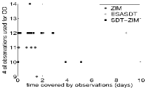
(d)

Figure 6: Time interval covered by the observations within the sets as a function of the number of observations used for orbit determination for object (a) E03174A, (b) E06321D, (c) E06327E and (d) E08241A.

Orbits were determined for different spacings of two observation sets stemming a) from one observation site only and b) from different sites. In the first case, the observations either stem from ZIMLAT or from ESASDT only. In the second case, not only the observations of ZIMLAT and ESASDT were combined but also observations of the ISON network, if available. When observations from different sites are used in orbit determination, the distribution is either that the first set of observations stems from one site and the second from another, or that there are observations from different sites at similar epochs used within the first and/or the last set of observations or a mixture of those options. In the figures the label ALL is applied, when observations of ZIMLAT (labeled ZIM), the ESASDT and of the ISON network are combined; the label SDT-ZIM is applied, if only the observations of ZIMLAT and the ESASDT are used. The distances between the observations and the ephemerides of the predicted orbits of the four objects for a prediction interval of 50 days after the last observation used for orbit determination were determined. The distances were averaged and a mean value and standard deviation was calculated. Between six and 50 single distances between ephemerides and observations were averaged.

The predicted ephemeris positions are compared to the optical angle-only observations, which were not used in orbit determination. Angular distances are determined on the celestial sphere. The observation used for the comparison stem from ZIMLAT and ESASDT and serve as ground truth. Calibration measurements with high accuracy ephemerides of Global Navigation Satellite System (GNSS) satellites provided by International GNSS Service (IGS) showed an accuracy of the measurements of ZIMLAT and ESASDT of below one arcsecond. That the further observations in fact belong to the same object is validated via an orbit determination with both the observations used in the original sparse data orbit determination and the observations, which they were compared to. An orbit determination with a root-mean-square of below two arcseconds is a reliable tool to associate observations of this accuracy of the same object to each other, as shown with cluster observations in Musci et al. , (2005).

2.2 Results

In Fig. 1 the angular distance between predicted and observed position are displayed as a function of the time interval between the first and the last observation, which were used in orbit determination. Displayed are the mean values and the standard deviations of the angular distances of the single orbits. The mean value and standard deviations are determined with the single angular distances of predicted position to observed ones, all within 50 days since orbit determination.

Figure 1 shows that the angular distances are in general very small. The vast majority of the determined orbits even produce distances smaller than 0.6 degrees. Except for the first object, each object also shows some outliers, with larger angular distances. These larger distances also tend to show larger standard deviations. The value of the angular distances seems to be, at least in this setup, quite independent of how large the difference between the first and the last observations of the fit interval is. Moreover, Figure 1 also shows that there is no significant difference in using observations only from one observation site for orbit determination or using observations from different sites. It could not be shown that the latter approach is more advantageous for orbit determination. Different observation sites still have advantages in terms of availability, weather conditions, which results in a larger amount of observations, which are available. In Fig. 2, the root mean square of the orbit determinations is shown, which were used for the prediction, as a function of the angular distance. No trend is visible, all orbits, which were determined had a small root mean square of below three arcseconds.

In Fig. 3, the angular distances are displayed as a function of the actual number of single observations that entered orbit determination. It can be seen that no strong correlation is visible between the actual number of observations used and the value for the distances.

To find a measure for the true anomaly distribution, an anomaly distribution measure $f_{\text{ano}}$ was defined: It would be ideal to distribute all $n$ observations equally spaced with an angle of $2\pi/n$ between each observation. The deviation from this ideal distribution is determined and normalized with the number of observations. The smaller $f_{\text{ano}}$, the better distributed are the observations in anomaly.

$$f_{\text{ano}}=\frac{1}{n}\sqrt{\sum_{i=1}^{n-1}\big{(}\frac{2\pi}{n}-(a_{i+1}-a_{i})\big{)}^{2}+\big{(}\frac{2\pi}{n}-(a_{1}+2\pi-a_{n})\big{)}^{2}},$$ (2)

where as $n$ is the number of observations and $a_{i}$ with $i=1,..,n$ are the anomalies of the single observations, in ascending anomaly order. The angular distances as a function of $f_{\text{ano}}$ are displayed in Fig. 4. There is no clear correlation between the $f_{\text{ano}}$ and the distances, as it is expected for objects with small eccentricities. Object E06327E, with the highest eccentricity of e=0.06, has the strongest correlation with $f_{\text{ano}}$.

The crucial factor however, seems to be the time interval covered by observations itself within the sets. In Fig 5, the angular distances are displayed as a function of the time interval covered within the two sets used in the beginning and the end of the fit interval, without the time gap in between the two sets. A strong correlation is visible. Fig. 6 shows that there is no strong correlation between the number of used observations and the time interval covered within the sets. For example for the ESASDT observation strategy, primarily densely spaced observations are available.

The investigation of the data displayed in Fig. 6 showed that a coverage of at least 1.2 hours for both sets together seems to be necessary, in order to gain an orbit which allows to safely re-detect the investigated objects in more than 90 percent of all cases with a field of view of one square degree, that is to have an accuracy of below 0.5 degrees.

[ht]

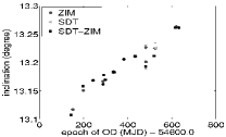
(a)

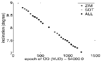
(b)

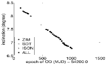
(c)

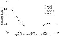
(d)

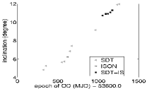
(e)

Figure 7: Inclination as a function of time for orbits of the object (a)E08241A, (b) E06321D, (c) E07194A, (d) E07308B, (e) E06293A.

[h]

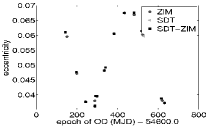
(a)

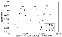
(b)

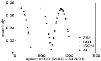
(c)

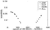
(d)

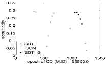
(e)

Figure 8: Eccentricity as a function of time for orbits of the object (a) E08241A, (b) E06321D, (c) E07194A, (d) E07308B, (e) E06293A.

3 Investigation of HAMR Objects in Sparse Data Setup

The dynamical properties of HAMR objects were studied in the normalized sparse data setup established in the previous section. Orbits are determined with two observation sets only. The sets consist of four to eight observations each. The observations are required to span at least a time interval of 1.2 hours within the sets and need to be well spread over the anomaly for the objects in orbits with a high eccentricity. The total fit interval for orbit determination ranges between 10 and 120 days. As shown in the previous section the comparability of the orbits do not seem to be dependent on these ranges.

The orbits were first determined with observations from one observation site only, then with observations from different sites in the setup mentioned above. The observations used in this investigation stem from the ESASDT, ZIMLAT, and from several telescopes of the ISON network.

3.1 Selected Objects

Five objects were selected for a detailed investigation. All objects were discovered and first detected by the AIUB and are not listed in the USSTRATCOM catalogue. All objects are faint debris objects. They were tracked successfully over several years, and no maneuvers were detected. A set of osculating orbital elements and an average value for the apparent magnitudes are listed in Tab. 2. The two objects with the lowest AMR values, E08241A and E06321D, which were used in the investigation of the sparse data orbit determination, are used here again.

Table 2: Investigated HAMR objects: Internal name, epoch (MJD), eccentricity, inclination (deg), semi-major axis (km), area to mass ratio ($m^{2}/kg$) and apparent magnitude (mag).

NAME	Epoch	a	e	i	AMR	Mag
E08241A	55213.0	41600	0.041	13.26	1.24	16.1
E06321D	55275.9	41400	0.035	7.00	2.29	15.3
E07194A	54877.0	40900	0.005	7.31	3.37	16.8
E07308B	54416.0	35600	0.264	7.63	8.83	15.8
E06293A	54951.0	40200	0.245	11.06	15.41	16.8

[ht]

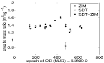
(a)

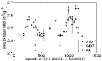
(b)

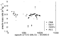
(c)

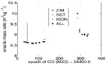
(d)

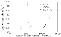
(e)

Figure 9: AMR as a function of time for orbits of the object (a) E08241A, (b) E06321D, (c) E07194A, (d) E07308B, (e) E06293A.

[h]

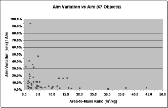
(a)

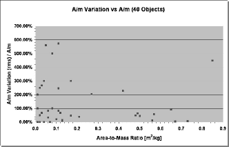
(b)

Figure 10: Relative variation of AMR value as a function of the absolute AMR value of (a) 47 HAMR and (b) LAMR objects.

[h]

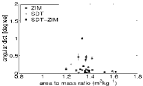
(a)

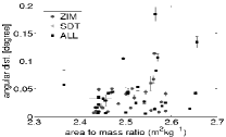
(b)

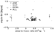
(c)

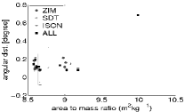
(d)

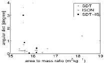
(e)

Figure 11: Angular distances of predicted orbits on the celestial sphere as a function of AMR for orbits of the object (a) E08241A, (b) E06321D, (c) E07194A, (d) E07308B, (e) E06293A.

[h]

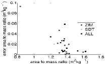
(a)

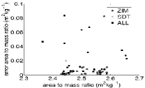
(b)

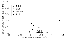
(c)

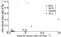
(d)

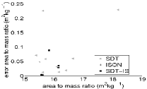
(e)

Figure 12: Error of the AMR value as a function of AMR as estimated in orbits of the object (a) E08241A, (b) E06321D, (c) E07194A, (d) E07308B, (e) E06293A.

[h]

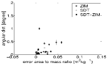
(a)

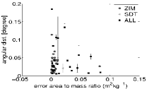
(b)

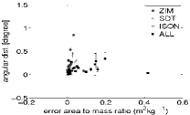
(c)

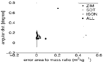
(d)

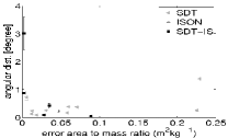
(e)

Figure 13: Absolute values and standard deviations of the angular distances as a function of the error of the AMR value as found in orbit determination of the object (a) E08241A, (b) E06321D, (c) E07194A, (d) E07308B, (e) E06293A.

3.2 Evolution of Orbital Elements

The evolution of the orbital elements over time is inspected in a first step. Figure 7 shows the development of the inclination and its errors in inclination, of the five objects. The error bars are too small, to be visible in the plot in most cases. The inclination values of the different orbits are closely aligned to each other and mark a consistent evolution, only in the case of object E08241A in Fig. 7 a wider spread in the inclination values can be observed. The orbits determined with observations from the different observation sites produce almost identical results. For object E07308B and E06293A, which have the highest AMR values, the inclination seems not to follow a steady increase over time, but some smaller periodic substructure seems to be superimposed. These may very well be the perturbations with a period of one nodal year, which are well known for objects with high AMR, see e.g., Liou & Weaver, (2005), Schildknecht et al. , (2005b).

Figure 8 shows the evolution of the eccentricity values and its errors estimated in orbit determination for the different objects. Periodic variations can be observed for all objects. The different orbits with observations from one site only or from different sites result in the same eccentricities.

3.3 Evolution of Area to Mass Ratio Value

Figure 9 shows the AMR values as a function of time for the objects listed in Tab. 2. In all cases, the values for the AMR do not show clear and obvious common trends, see Fig. 7 and 8.

For object E08241A, the AMR values vary around a mean value of 1.4 $\text{m}^{2}\text{kg}^{-1}$ with no obvious trend or periodic signal, see Fig. 9a.

For object E06321D (see Fig. 9b), the AMR value seems to vary periodically with a period of about one year around a value of 2.5 $\text{m}^{2}\text{kg}^{-1}$, but also values of 2.35 $\text{m}^{2}\text{kg}^{-1}$ and 2.65 $\text{m}^{2}\text{kg}^{-1}$ occur. Similar results were obtained by Musci et al. , (2010), for the same object, in different orbit determination setups. The AMR value of object E07194A (see Fig. 9c) varies around 3.5 $\text{m}^{2}\text{kg}^{-1}$, but in the orbits determined with combined observations from all the sites, so-called outliers of 4.5 $\text{m}^{2}\text{kg}^{-1}$ and 2.3 $\text{m}^{2}\text{kg}^{-1}$ occur as well. These have, however large error values.

Object E07308B (see Fig. 9d) seems to generally increase its AMR value over time from a value of 8.5 $\text{m}^{2}\text{kg}^{-1}$ up to 9.0 $\text{m}^{2}\text{kg}^{-1}$. But single orbits also show AMR values of i.e. 10 $\text{m}^{2}\text{kg}^{-1}$.

Figure 9e shows that object E06293A, which is the object with the largest AMR value regarded here, has significant data gaps. A general trend of the AMR value in time, increasing from 15.5 $\text{m}^{2}\text{kg}^{-1}$ to 16.5 $\text{m}^{2}\text{kg}^{-1}$ cannot be excluded. But one orbit determined with ESASDT data also shows a value of 18.2 $\text{m}^{2}\text{kg}^{-1}$, with a small formal error.

No general correlation between the AMR value itself and the variations of the AMR value could be determined, no general trend is visible. A study on the variation of AMR values was conducted by Schildkecht et al. , (to be published 2011). The variations of the AMR values of 47 HAMR objects were investigated and compared to the AMR variations of orbits of 40 low AMR (LAMR) value objects. No normalized or sparse data setup orbit determination setup was chosen. The AMR values in that analysis were determined in the standard orbit determination procedure at the AIUB, with fit arcs as long as possible for a successful, that is defined as leading to a small rms error, orbit determination. The results are illustrated in Fig. 10. No general trend in the AMR variations could be determined for either HAMR or LAMR objects. The relative variations of the AMR values of the LAMR objects were larger, than the AMR variations of the HAMR values. The AMR variations of the LAMR objects were of the order of several 100 percent.

All orbits were predicted and compared to additional observations of the same object, which were not used for orbit determination. The additional observations were all checked via orbit determination, to ensure that they belong to the same object. Figure 11 shows the angular distances between the predicted ephemeris and observations. The values are averaged over all distances 50 days after orbit determination and their standard deviations serve as error bars.

Figure 11a shows that for object E08241A, one orbit produces the largest distances of one degree. This orbit does not show up prominently in the orbital parameter plots (see Fig. 8a and 7a) or AMR value plots (see Fig. 9a). The orbit with ZIMLAT data, which produced the outlier AMR value of 0.82$\text{m}^{2}\text{kg}^{-1}$, does not show up prominently in the distance plot (Fig. 11a).

The mean value of all angular distances of object E06321D are well below 0.2 degrees, but four orbits show large standard deviations in the angular distance, as Fig. 11b shows. All of them have been determined with combined observations from ZIMLAT, ESASDT, and ISON observations. Their AMR values are 2.36 $m^{2}kg^{-1}$, 2.50 $\text{m}^{2}\text{kg}^{-1}$, 2.57 $\text{m}^{2}\text{kg}^{-1}$, and 2.66 $\text{m}^{2}\text{kg}^{-1}$. The orbits with the AMR value of 2.36 $\text{m}^{2}\text{kg}^{-1}$ does show up also in a group of outlier AMR values, which do not seem to follow the periodic variation in the evolution of the AMR values. The other orbits, with large standard variations in the angular distance do not show up prominently (Fig. 9b). Those orbits with the largest standard variation in angular distance do not show the largest error in the AMR values either, as Fig. 13 shows.

Figure 11c shows for object E07194A three angular distances with large standard deviations. The orbits were determined with observations from all sites. They have AMR values of 2.12 $\text{m}^{2}\text{kg}^{-1}$, 2.21 $\text{m}^{2}\text{kg}^{-1}$, and 4.46 $\text{m}^{2}\text{kg}^{-1}$. Those are the smallest and largest AMR values in the determined orbits for E07194A. These three values do also show up as outliers in Fig. 9c. For objects E07308B and E06293A, the angular distances with a large standard variation (see Fig. 11d and e), do not show significant outlier AMR values in Fig. 9d and e. For object E07308B, the orbit with an AMR value of 10.15 $\text{m}^{2}\text{kg}^{-1}$ shows the largest mean value in the angular distance of almost 0.7 degrees but has a small standard deviation in this distance (Fig. 11d). This value is significantly different compared to the other determined AMR values, see Fig. 9d.

The dependency of the AMR value on the error of the AMR, as it was found in orbit determination, is investigated in the final step. No clear correlation could be determined between the AMR value and its rms value (Fig. 12).

Figure 13 shows the angular distance distances on the celestial sphere as a function of the error of the AMR value. As expected, for none of the objects a clear correlation between the error of the AMR value and the absolute value of the distances or the standard deviation of the distances could be determined.

All investigated objects show variations in the AMR value, but not a common characteristic in these variations. It has to be noted that the result may be affected by the relatively simple shadowing model that was used in orbit determination; as it was shown Pardini & Anselmo, (2008), Valk & Lemaître, (2008), shadowing effects have a significant influence on the long term evolution of orbits of HAMR objects. Investigation of simulated orbits with numerical and semi-analytical methods, e.g. by Valk & Lemaître, (2008), Valk et al. , (2008) also showed the existence of irregular chaotic orbits and the significant influence of secondary resonances on the orbits of HAMR objects. However, these simulations did assume a constant AMR value. Complex attitude motion, irregular shapes, and/or deformation of the actual objects, could lead to an actual change in the AMR value itself over time, which may not be averaged out over the fit interval of orbit determination.

4 Conclusions

A sparse data setup was established to create comparable orbits over longer time intervals. Orbits with two data sets only do produce small differences between the propagated ephemerides and further observations, as long as 1.2 hours are covered within the sets. Other factors, such as that the observations stem from different sites or the time interval between the sets, are found to be negligible.

The orbits of high area-to-mass ratio (HAMR) objects were analyzed in this setup. The AMR value, that is the scaling factor of the direct radiation pressure (DRP) parameter, varies over time. The order of magnitude of the variation of the area-to-mass ratio (AMR) value was not correlated with the order of magnitude of its error.

The variation of the AMR is not averaged out in the fit interval of orbit determination. In the evolution of the AMR value over time, no common characteristic could be determined for different HAMR objects. Further work on the orbits of HAMR objects is needed, to improve the radiation pressure model, to determine possible attitude motion or deformations and to understand also resonance effects and the existence of chaotic regions.

References

- Beutler, (2005) Beutler, G. 2005. Methods of Celestial Mechanics. Two Volumes. Springer-Verlag, Heidelberg. ISBN: 3-540-40749-9 and 3-540-40750-1.
- Liou & Weaver, (2005) Liou, J.-C., & Weaver, J.K.2̇005. Orbital Dynamics of High Area-to-Mass Ratio Debris and Their Distribution in the Geosynchronos Region. In: Proceedings of the Forth European Conference on Space Debris, pp. 119-124, ESOC, Darmstadt, Germany, 18-20 April 2005.
- Musci et al. , (2005) Musci, R., Schildknecht, T. Flohrer, T. & Beutler, G.2̇005. Concept for a Catalogue of Space Debris in GEO. In: Proceedings of the Fourth European Conference on Space Debris, pp. 601-606, ESOC, Darmstadt, Germany, 18-20 April 2005.
- Musci et al. , (2010) Musci, R., Schildknecht, T. & Ploner, M.2̇010. Analyzing long Observation Arcs for Objects with high Area-to-Mass Ratios in Geostationary Orbits. In: Acta Astronautica, vol. 66, pp 693-703.
- Pardini & Anselmo, (2008) Pardini, C., & Anselmo, L.2̇008. Long-Term Evolution of Geosynchronous Orbital Debris with High Area-to-Mass Ratios. Trans. Japan Soc. Aero. Space Sci., 51, 22–27.
- Schildkecht et al. , (to be published 2011) Schildkecht, T., Früh, C. Hinze, A. & Herzog, J.ṫo be published 2011. Dynamical Properties of High Area to Mass Ratio Objects in GEO-Like Orbits. Advances in Space Research.
- Schildknecht et al. , (2003) Schildknecht, T., Musci, R. Ploner, M. Flury, W. Kuusela, J. de León Cruz, J. & de Fatima Domínguez Palmero, L.2̇003. An Optical Search for Small-Size Debris in GEO and GTO. In: Proceedings of the 2003 AMOS Technical Conference, 9-12 September 2003, Maui, Hawaii, USA.
- Schildknecht et al. , (2004) Schildknecht, T., Musci, R. Ploner, M. Beutler, G. Kuusela, J. de León Cruz, J. & de Fatima Domínguez Palmero, L.2̇004. Optical Observations of Space Debris in GEO and in Highly-Eccentric Orbits. Advances in Space Research, 34(5), 901–911.
- Schildknecht et al. , (2005a) Schildknecht, T., Musci, R. Flury, W. Kuusela, J. de León Cruz, J. & de Fatima Domínguez Palmero, L.2̇005a. Optical Observations of Space Debris in High-Altitude Orbits. In: Proceedings of the Forth European Conference on Space Debris, pp. 113-118, ESOC, Darmstadt, Germany, 18-20 April 2005.
- Schildknecht et al. , (2005b) Schildknecht, T., Musci, R. Flury, W. Kuusela, J. de León Cruz, J. & de Fatima Domínguez Palmero, L.2̇005b. Properties of the High Area-to-Mass Ratio Space Debris Population in GEO. In: Proceedings of the 2005 AMOS Technical Conference, 5-9 September 2005, Maui, Hawaii, USA.
- Valk & Lemaître, (2008) Valk, S., & Lemaître, A.2̇008. Semi-Analytical Investigations of High Area-to-Mass Ratio geosynchronous Space Debris Including Earth’s Shadowing Effects. Advances in Space Research, 42(8), 1429–1443.
- Valk et al. , (2008) Valk, S., Delsate, N. Lemaître, A. & Carletti, T.2̇008. Semi-Analytical Investigations of High Area-to-Mass Ratio geosynchronous Space Debris Including Earth’s Shadowing Effects. Advances in Space Research, 43(10), 1509–1526.
- Vallado & McCain, (2001) Vallado, D., & McCain, W.2̇001. Fundmentals of Astrodynamics and Applications. Microcosm Press, El Segundo, California. ISBN 0-7923-6903-3.