{psinputs}

Focusing mKdV breather solutions with nonvanishing boundary conditions by the Inverse Scattering Method

Miguel A. Alejo Departament of Theoretical Biology, University of Bonn
Germany
miguel.alejo@uni-bonn.de
(Date: September, 2011)
Abstract.

Using the Inverse Scattering Method with a nonvanishing boundary condition, we obtain the square $k^{2}$ of a focusing modified Korteweg-de Vries (mKdV) breather solution with non zero vacuum parameter $b^{2}$. We are able to factorize and simplify it in order to get explicitly the associated mKdV breather solution $k$ with non zero vacuum parameter $b$. Moreover, taking the limiting case of zero frequency, we obtain a generalization of the Double Pole solution introduced by M.Wadati et al.

Key words and phrases:
mKdV equation, Breather, inverse scattering, nonvanishing condition
2000 Mathematics Subject Classification:
Primary 37K15, 35Q53; Secondary 35Q51, 37K10

1. Introduction

The focusing modified Korteweg-de Vries equation (mKdV for short)

βˆ‚kβˆ‚t+βˆ‚kβˆ‚s3+6​k2β€‹βˆ‚kβˆ‚s=0,(s,t)βˆˆβ„Γ—β„.formulae-sequenceπ‘˜π‘‘π‘˜superscript𝑠36superscriptπ‘˜2π‘˜π‘ 0𝑠𝑑ℝℝ\frac{\partial k}{\partial t}+\frac{\partial k}{\partial s^{3}}+6k^{2}\frac{\partial k}{\partial s}=0,\leavevmode\nobreak\ \leavevmode\nobreak\ (s,t)\in\mathbb{R}\times\mathbb{R}. (1.1)

appears to be relevant in a number of different physical systems (e.g. phonons in anharmonic lattices, models of traffic congestion, curve motion and fluid mechanics between others). Indeed, it can also be considered as a canonical equation, as KdV, sine-Gordon and non linear SchrΓΆdinger equations.

Breather solutions of mKdV (1.1) in the line were found by M.Wadati [13] (see also G.Lamb [10]). They were rediscovered by C.Kenig, G.Ponce and L.Vega in the proof of the discontinuity of the flowmaps associated to mKdV equation in the Sobolev spaces $H^{\sigma}$, constituted by functions with $\sigma$ derivatives in $L^{2}(\mathbb{R})$ (see [9]). Those breather solutions are defined in all the real line, vanish exponentially at infinity and, in a qualitative point of view, describe traveling wave packets.

Indeed, they are determined by four real parameters, two of them given by the amplitude ($\beta$) of the envelope and the frequency ($\alpha$) of the carried wave and the other two given by time and spatial translations (represented by $u_{0},v_{0}$ below). It is well known that such breather solutions can be written as follows

k​(s,t)=βˆ’iβ€‹βˆ‚βˆ‚s​log⁑(f​(u)+i​g​(v)f​(u)βˆ’i​g​(v))=2β€‹βˆ‚βˆ‚s​arctan⁑(g​(v)f​(u)),π‘˜π‘ π‘‘π‘–π‘ π‘“π‘’π‘–π‘”π‘£π‘“π‘’π‘–π‘”π‘£2𝑠𝑔𝑣𝑓𝑒k(s,t)=-i\frac{\partial}{\partial s}\log\left(\frac{f(u)+ig(v)}{f(u)-ig(v)}\right)=2\frac{\partial}{\partial s}\arctan\left(\frac{g(v)}{f(u)}\right), (1.2)

where $u=2\beta s+\gamma t+u_{0}$,Β Β  v=2​α​s+δ​t+v0𝑣2𝛼𝑠𝛿𝑑subscript𝑣0v=2\alpha s+\delta t+v_{0},Β Β Ξ³=8​β​(βˆ’Ξ²2+3​α2)𝛾8𝛽superscript𝛽23superscript𝛼2\gamma=8\beta(-\beta^{2}+3\alpha^{2}),Β Β  Ξ΄=8​α​(Ξ±2βˆ’3​β2)𝛿8𝛼superscript𝛼23superscript𝛽2\delta=8\alpha(\alpha^{2}-3\beta^{2}), and111The $arctan$ phase in the argument of $g$ can be dropped with a suitable translation in time and space, but it will not be done for comparison purposes.

$\displaystyle g(v)$ $\displaystyle=$ $\displaystyle\frac{\beta}{\alpha}\sin\left(v-\arctan\left(\frac{\beta}{\alpha}\right)\right),$ (1.3)
$\displaystyle f(u)$ $\displaystyle=$ $\displaystyle\cosh(u).$ (1.4)

This paper is devoted to the use of the Inverse Scattering Method (ISM for short) under a nonvanishing boundary condition(NVBC shortly) devised by T.Kawata and H.Inoue [8] to obtain breather solutions of mKdV (1.1) which at infinity behave as a non trivial constant parameter $b$. The interest of this kind of solutions of the mKdV is related with the problem of the evolution of closed planar curves under the mKdV flow in the following way. By the work of R.Goldstein and D.Petrich [6] the equation (1.1) is considered as the evolution equation of the curvature of a curve. By this work, closed curves can be considered as those whose associated curvature satisfies that its mean is non-zero. Moreover, those curvatures can be obtained from a solution of the focusing mKdV constructed by the (nonlinear) superposition of a constant (e.g. constant $b$) plus a traveling wave. In fact, it is posible to find some special breather solutions associated to simple closed curves that, when evolving under the mKdV flow, they create and annihilate self-intersections (see [2] for more information).

Although in the literature some kind of breather solutions of the Gardner equation(also known as the extended KdV equation) have been obtained before [7, 12], they do not contain details on derivations of these breather solutions from the ISM scheme. Even despite the close relation between Gardner and mKdV equations (solutions of the mKdV equation with NVBC are also solutions of the Gardner equation with zero boundary condition), breathers obtained in these references [7, 12] are far to be easily compared with the breather of M.Wadati [13] they generalize. These two aspects are attained too in the present paper(for further details see section 2.2 and (2.47)). Finally note that the mKdV breather solutions mentioned above can be obtained alternatively using the Hirota method with a suitable selection of the wavenumbers (see the work of K.Chow and D.Lai [5]).

2. Breather solutions of the focusing mKdV with nonvanishing boundary conditions

In this section we obtain breathers of the focusing mKdV (1.1) with nonvanishing boundary conditions by using the ISM for potentials that are not trivial at infinity, introduced by T.Kawata and H.Inoue in [8]. We also recall the work of T.Au-Yeung et al.[4], in which the same approach was used to obtain one and two soliton solutions with non trivial values at infinity. First, we summarize some basic results from [8] and [4], necessary for our research.

2.1. Basic results of T.Kawata and H.Inoue for the mKdV

T.Kawata and H.Inoue considered in [1] a generalized AKNS eigenvalue problem for nonvanishing potentials, which consist in the following spatial and time evolution equations111In what follows, subindices of the form ${f}_{s}$ means $\partial_{s}f\equiv\frac{\partial f}{\partial s}$.:

𝐯s=D​(Ξ»)​𝐯,D​(Ξ»;s,t)=(βˆ’i​λq​(s,t)r​(s,t)i​λ),formulae-sequencesubscriptπ―π‘ π·πœ†π―π·πœ†π‘ π‘‘matrixπ‘–πœ†π‘žπ‘ π‘‘π‘Ÿπ‘ π‘‘π‘–πœ†{\bf v}_{s}=D(\lambda){\bf v},\leavevmode\nobreak\ \leavevmode\nobreak\ D(\lambda;s,t)=\begin{pmatrix}-i\lambda&q(s,t)\\ r(s,t)&i\lambda\end{pmatrix}, (2.1)
𝐯t=F​(Ξ»)​𝐯,F​(Ξ»;s,t)=(A​(Ξ»)B​(Ξ»)C​(Ξ»)βˆ’A​(Ξ»)),formulae-sequencesubscriptπ―π‘‘πΉπœ†π―πΉπœ†π‘ π‘‘matrixπ΄πœ†π΅πœ†πΆπœ†π΄πœ†{\bf v}_{t}=F(\lambda){\bf v},\leavevmode\nobreak\ \leavevmode\nobreak\ F(\lambda;s,t)=\begin{pmatrix}A(\lambda)&B(\lambda)\\ C(\lambda)&-A(\lambda)\end{pmatrix}, (2.2)

where

A​(Ξ»)=βˆ’4​i​λ3βˆ’2​i​λ​q​r+r​qsβˆ’q​rs,B​(Ξ»)=4​λ2​q+2​i​λ​qs+2​q2​rβˆ’qs​s,C​(Ξ»)=4​λ2​rβˆ’2​i​λ​r+2​q​r2βˆ’rs​s.π΄πœ†4𝑖superscriptπœ†32π‘–πœ†π‘žπ‘Ÿπ‘Ÿsubscriptπ‘žπ‘ π‘žsubscriptπ‘Ÿπ‘ missing-subexpressionmissing-subexpressionmissing-subexpressionmissing-subexpressionmissing-subexpressionπ΅πœ†4superscriptπœ†2π‘ž2π‘–πœ†subscriptπ‘žπ‘ 2superscriptπ‘ž2π‘Ÿsubscriptπ‘žπ‘ π‘ missing-subexpressionmissing-subexpressionmissing-subexpressionmissing-subexpressionmissing-subexpressionπΆπœ†4superscriptπœ†2π‘Ÿ2π‘–πœ†π‘Ÿ2π‘žsuperscriptπ‘Ÿ2subscriptπ‘Ÿπ‘ π‘ missing-subexpressionmissing-subexpression\begin{array}[]{lll}A(\lambda)=-4i\lambda^{3}-2i\lambda qr+rq_{s}-qr_{s},\\ \\ B(\lambda)=4\lambda^{2}q+2i\lambda q_{s}+2q^{2}r-q_{ss},\\ \\ C(\lambda)=4\lambda^{2}r-2i\lambda r+2qr^{2}-r_{ss}.\end{array} (2.3)

Matrices $D(\lambda)$ and $F(\lambda)$ satisfy the well known integrable condition associated to equations (2.1) and (2.2) (i.e $\partial_{t}$(2.1)$=\partial_{s}$(2.2)):

$$D_{t}-F_{s}+DF-FD=0.$$ (2.4)

They seek a real potential solution q​(s,t)π‘žπ‘ π‘‘q(s,t) under the following boundary condition:

q​(s,t)β†’bassβ†’Β±βˆž;b2=βˆ’Ξ»02,formulae-sequenceβ†’π‘žπ‘ π‘‘π‘asformulae-sequence→𝑠plus-or-minussuperscript𝑏2superscriptsubscriptπœ†02q(s,t)\rightarrow b\leavevmode\nobreak\ \leavevmode\nobreak\ \leavevmode\nobreak\ \text{as}\leavevmode\nobreak\ \leavevmode\nobreak\ \leavevmode\nobreak\ s\rightarrow\pm\infty;\leavevmode\nobreak\ \leavevmode\nobreak\ b^{2}=-\lambda_{0}^{2}, (2.5)

requiring that q​(s,t)π‘žπ‘ π‘‘q(s,t) is sufficiently smooth and all the $s$ derivatives of $q$ tend to zero as sβ†’Β±βˆžβ†’π‘ plus-or-minuss\rightarrow\pm\infty. For this purpose, they consider potentials q​(s,t)π‘žπ‘ π‘‘q(s,t) and r​(s,t)π‘Ÿπ‘ π‘‘r(s,t) with the following nonvanishing conditions:

q​(s,t)​(orr​(s,t))β†’q±​(orrΒ±)assβ†’Β±βˆž,q+​r+=qβˆ’β€‹rβˆ’=Ξ»02,formulae-sequenceβ†’π‘žπ‘ π‘‘orπ‘Ÿπ‘ π‘‘superscriptπ‘žplus-or-minusorsuperscriptπ‘Ÿplus-or-minusas→𝑠plus-or-minusmissing-subexpressionmissing-subexpressionmissing-subexpressionmissing-subexpressionmissing-subexpressionsuperscriptπ‘žsuperscriptπ‘Ÿsuperscriptπ‘žsuperscriptπ‘Ÿsuperscriptsubscriptπœ†02missing-subexpressionmissing-subexpression\begin{array}[]{lll}q(s,t)(\text{or}\leavevmode\nobreak\ \leavevmode\nobreak\ r(s,t))\rightarrow q^{\pm}(\text{or}\leavevmode\nobreak\ \leavevmode\nobreak\ r^{\pm})\leavevmode\nobreak\ \leavevmode\nobreak\ \leavevmode\nobreak\ \text{as}\leavevmode\nobreak\ \leavevmode\nobreak\ \leavevmode\nobreak\ s\rightarrow\pm\infty,\\ \\ q^{+}r^{+}=q^{-}r^{-}=\lambda_{0}^{2},\end{array} (2.6)

where $q^{\pm},r^{\pm}$ and $\lambda_{0}^{2}$ are constants. Then, the spatial evolution matrix D​(Ξ»;s,t)π·πœ†π‘ π‘‘D(\lambda;s,t) can be written as follows:

D​(Ξ»;s,t)=D±​(Ξ»)+Δ​D±​(s,t),π·πœ†π‘ π‘‘superscript𝐷plus-or-minusπœ†Ξ”superscript𝐷plus-or-minus𝑠𝑑D(\lambda;s,t)=D^{\pm}(\lambda)+\Delta D^{\pm}(s,t), (2.7a)
D±​(Ξ»)=limsβ†’Β±βˆžD​(Ξ»;s,t)=(βˆ’i​λqΒ±rΒ±i​λ),superscript𝐷plus-or-minusπœ†subscript→𝑠plus-or-minusπ·πœ†π‘ π‘‘matrixπ‘–πœ†superscriptπ‘žplus-or-minussuperscriptπ‘Ÿplus-or-minusπ‘–πœ†D^{\pm}(\lambda)=\lim_{s\rightarrow\pm\infty}D(\lambda;s,t)=\begin{pmatrix}-i\lambda&q^{\pm}\\ r^{\pm}&i\lambda\end{pmatrix}, (2.7b)
Δ​D±​(s,t)=D​(Ξ»;s,t)βˆ’D±​(Ξ»)=(0q​(s,t)βˆ’qΒ±r​(s,t)βˆ’rΒ±0),Ξ”superscript𝐷plus-or-minusπ‘ π‘‘π·πœ†π‘ π‘‘superscript𝐷plus-or-minusπœ†matrix0π‘žπ‘ π‘‘superscriptπ‘žplus-or-minusπ‘Ÿπ‘ π‘‘superscriptπ‘Ÿplus-or-minus0\Delta D^{\pm}(s,t)=D(\lambda;s,t)-D^{\pm}(\lambda)=\begin{pmatrix}0&q(s,t)-q^{\pm}\\ r(s,t)-r^{\pm}&0\end{pmatrix}, (2.7c)

and the characteristic roots of $D^{\pm}(\lambda)$ are $\pm i\zeta$, with $\zeta=\sqrt{\lambda^{2}-\lambda_{0}^{2}}$. Now, they define

T±​(Ξ»,ΞΆ)=limsβ†’Β±βˆžT​(Ξ»,ΞΆ;s),superscript𝑇plus-or-minusπœ†πœsubscript→𝑠plus-or-minusπ‘‡πœ†πœπ‘ missing-subexpression\begin{array}[]{ll}T^{\pm}(\lambda,\zeta)=\lim_{s\rightarrow\pm\infty}T(\lambda,\zeta;s),\end{array} (2.8)

where

T​(Ξ»,ΞΆ;s)=(βˆ’i​q1​(s)Ξ»βˆ’ΞΆΞ»βˆ’ΞΆi​r1​(s)),π‘‡πœ†πœπ‘ matrix𝑖subscriptπ‘ž1π‘ πœ†πœπœ†πœπ‘–subscriptπ‘Ÿ1𝑠T(\lambda,\zeta;s)=\begin{pmatrix}-iq_{1}(s)&\lambda-\zeta\\ \lambda-\zeta&ir_{1}(s)\end{pmatrix},

and $q_{1}$, $r_{1}$ are suitable smooth and satisfy that $q_{1}(s)r_{1}(s)=\lambda_{0}^{2}$ for all sβˆˆβ„π‘ β„s\in\mathbb{R}. The matrices $D^{\pm}(\lambda)$ can be diagonalized by $T^{\pm}(\lambda,\zeta)$ as

$$D^{\pm}(\lambda)=-i\zeta T^{\pm}(\lambda,\zeta)\sigma_{3}[T^{\pm}(\lambda,\zeta)]^{-1}.$$ (2.9)

Using (2.9), they can define Jost matrices $\Phi^{\pm}$ as the solutions of (2.1) under conditions

Φ±​(Ξ»,ΞΆ;s,t)β†’T±​(Ξ»,ΞΆ)​J​(΢​s)assβ†’Β±βˆž,formulae-sequenceβ†’superscriptΞ¦plus-or-minusπœ†πœπ‘ π‘‘superscript𝑇plus-or-minusπœ†πœπ½πœπ‘ as→𝑠plus-or-minus\Phi^{\pm}(\lambda,\zeta;s,t)\rightarrow T^{\pm}(\lambda,\zeta)J(\zeta s)\leavevmode\nobreak\ \leavevmode\nobreak\ \text{as}\leavevmode\nobreak\ \leavevmode\nobreak\ s\rightarrow\pm\infty, (2.10)

where

J​(΢​s)=(eβˆ’i​΢​s00ei​΢​s).π½πœπ‘ matrixsuperscriptπ‘’π‘–πœπ‘ 00superscriptπ‘’π‘–πœπ‘ J(\zeta s)=\begin{pmatrix}e^{-i\zeta s}&0\\ 0&e^{i\zeta s}\end{pmatrix}.

Then, a scattering matrix $S$ is defined by

Ξ¦βˆ’β€‹(Ξ»,ΞΆ;s,t)=Ξ¦+​(Ξ»,ΞΆ;s,t)​S​(Ξ»,ΞΆ;t),superscriptΞ¦πœ†πœπ‘ π‘‘superscriptΞ¦πœ†πœπ‘ π‘‘π‘†πœ†πœπ‘‘\Phi^{-}(\lambda,\zeta;s,t)=\Phi^{+}(\lambda,\zeta;s,t)S(\lambda,\zeta;t), (2.11)

and using relations (2.2),(2.9), (2.11) it is easy to derive the following condition:

$$S_{t}+SW^{-}-W^{+}S=0,\leavevmode\nobreak\ \leavevmode\nobreak\ S|_{t=0}=S_{0},$$ (2.12)

where $S_{0}$ is given by the direct scattering, and

WΒ±=΢​σ3β‹…βˆ‘n=1Nan​λnβˆ’1+i​(a0/ΞΆ)​(βˆ’i​λr±​e2​i​΢​sq±​eβˆ’2​i​΢​si​λ).superscriptπ‘Šplus-or-minusβ‹…πœsubscript𝜎3superscriptsubscript𝑛1𝑁subscriptπ‘Žπ‘›superscriptπœ†π‘›1𝑖subscriptπ‘Ž0𝜁matrixπ‘–πœ†superscriptπ‘Ÿplus-or-minussuperscript𝑒2π‘–πœπ‘ superscriptπ‘žplus-or-minussuperscript𝑒2π‘–πœπ‘ π‘–πœ†W^{\pm}=\zeta\sigma_{3}\cdot\sum_{n=1}^{N}a_{n}\lambda^{n-1}+i(a_{0}/\zeta)\begin{pmatrix}-i\lambda&r^{\pm}e^{2i\zeta s}\\ q^{\pm}e^{-2i\zeta s}&i\lambda\end{pmatrix}. (2.13)

The solution of (2.13) is easily obtained as follows

$$S(\lambda,\zeta;t)=e^{W^{+}t}S_{0}(\lambda,\zeta)e^{-W^{-}t}.$$ (2.14)

At this point, we apply this framework to the mKdV equation (1.1), by choosing q​(s,t)=k​(s,t)π‘žπ‘ π‘‘π‘˜π‘ π‘‘q(s,t)=k(s,t) and r​(s,t)=βˆ’q​(s,t)π‘Ÿπ‘ π‘‘π‘žπ‘ π‘‘r(s,t)=-q(s,t). Then, we calculate from (2.13) the temporal evolution of the elements of the scattering matrix $(S_{ij})$. For that purpose (see [8, p.1723]), we select $N=3$ and $a_{0}=a_{2}=0$, $a_{1}=2ib^{2},\leavevmode\nobreak\ a_{3}=-4i$ in (2.13), so that:

$$S_{11}(\lambda,\zeta;t)=S_{11}(\lambda,\zeta;0),\hskip 14.22636ptS_{12}(\lambda,\zeta;t)=S_{12}(\lambda,\zeta;0)e^{-4i\zeta(2\lambda^{2}-b^{2})t},$$
$$S_{21}(\lambda,\zeta;t)=S_{21}(\lambda,\zeta;0)e^{4i\zeta(2\lambda^{2}-b^{2})t},\hskip 14.22636ptS_{22}(\lambda,\zeta;t)=S_{22}(\lambda,\zeta;0).$$

Now, assume that zeros of the $S_{11}(\lambda,\zeta;0)$ matrix element in the region $\Im(\zeta)>0$ are $(\lambda_{j},\zeta_{j}),\leavevmode\nobreak\ \leavevmode\nobreak\ j=1,2$ where

$$\zeta_{j}=\sqrt{\lambda_{j}^{2}+b^{2}},\leavevmode\nobreak\ \leavevmode\nobreak\ j=1,2,\leavevmode\nobreak\ \leavevmode\nobreak\ \text{for}\leavevmode\nobreak\ \leavevmode\nobreak\ \leavevmode\nobreak\ y>s,$$ (2.15)

and define the functions $K^{\pm}(s,y)$ as those satisfying the following three equations (for the shake simplicity, we drop the time dependence in $K^{\pm}$ and $H_{c}$ defined below):

βˆ‚KΒ±βˆ‚s​(s,y)+Οƒ3β€‹βˆ‚KΒ±βˆ‚y​(s,y)​σ3+Οƒ3​K±​(s,y)​σ3​[D±​(Ξ»)+i​λ​σ3]βˆ’(0k​(s,t)βˆ’k​(s,t)0)​K±​(s,y)=0,superscript𝐾plus-or-minus𝑠𝑠𝑦subscript𝜎3superscript𝐾plus-or-minus𝑦𝑠𝑦subscript𝜎3subscript𝜎3superscript𝐾plus-or-minus𝑠𝑦subscript𝜎3delimited-[]superscript𝐷plus-or-minusπœ†π‘–πœ†subscript𝜎3matrix0π‘˜π‘ π‘‘π‘˜π‘ π‘‘0superscript𝐾plus-or-minus𝑠𝑦0missing-subexpression\begin{array}[]{ll}\frac{\partial K^{\pm}}{\partial s}(s,y)+\sigma_{3}\frac{\partial K^{\pm}}{\partial y}(s,y)\sigma_{3}+\sigma_{3}K^{\pm}(s,y)\sigma_{3}[D^{\pm}(\lambda)+i\lambda\sigma_{3}]-\begin{pmatrix}0&k(s,t)\\ -k(s,t)&0\end{pmatrix}K^{\pm}(s,y)=0,\end{array} (2.16a)
Οƒ3​K±​(s,s)​σ3βˆ’K±​(s,s)+Δ​D±​(Ξ»;s,t)=0,subscript𝜎3superscript𝐾plus-or-minus𝑠𝑠subscript𝜎3superscript𝐾plus-or-minus𝑠𝑠Δsuperscript𝐷plus-or-minusπœ†π‘ π‘‘0\sigma_{3}K^{\pm}(s,s)\sigma_{3}-K^{\pm}(s,s)+\Delta D^{\pm}(\lambda;s,t)=0, (2.16b)
$$K^{\pm}(s,y)\rightarrow 0\leavevmode\nobreak\ \leavevmode\nobreak\ \text{as}\leavevmode\nobreak\ \leavevmode\nobreak\ y\rightarrow\pm\infty,$$ (2.16c)

where $D^{\pm}(\lambda)$ and Δ​D±​(Ξ»;s,t)Ξ”superscript𝐷plus-or-minusπœ†π‘ π‘‘\Delta D^{\pm}(\lambda;s,t) are defined by (2.7) and $\sigma_{3}\equiv\begin{pmatrix}1&0\\ 0&-1\end{pmatrix}$. Then, the Gelfand-Levitan equation reads as follows,

K+​(s,y)β‹…(01)+βˆ‘j=12(cjc~j)​ei​΢j​(s+y)βˆ’Hc​(s+y)​(01)βˆ’βˆ«s+∞K+​(s,yβ€²)β€‹βˆ‘j=12(cjc~j)​ei​΢j​(y+yβ€²)​d​yβ€²+∫s+∞K+​(s,yβ€²)​Hc​(s+yβ€²)​(01)​𝑑yβ€²=0,β‹…superscript𝐾𝑠𝑦01subscriptsuperscript2𝑗1subscript𝑐𝑗subscript~𝑐𝑗superscript𝑒𝑖subscriptπœπ‘—π‘ π‘¦subscript𝐻𝑐𝑠𝑦01missing-subexpressionmissing-subexpressionmissing-subexpressionsubscriptsuperscript𝑠superscript𝐾𝑠superscript𝑦′subscriptsuperscript2𝑗1subscript𝑐𝑗subscript~𝑐𝑗superscript𝑒𝑖subscriptπœπ‘—π‘¦superscript𝑦′𝑑superscript𝑦′subscriptsuperscript𝑠superscript𝐾𝑠superscript𝑦′subscript𝐻𝑐𝑠superscript𝑦′01differential-dsuperscript𝑦′0missing-subexpression\begin{array}[]{ll}K^{+}(s,y)\cdot\left(\begin{smallmatrix}0\\ 1\end{smallmatrix}\right)+\sum^{2}_{j=1}\left(\begin{smallmatrix}c_{j}\\ \tilde{c}_{j}\end{smallmatrix}\right)e^{i\zeta_{j}(s+y)}-H_{c}(s+y)\left(\begin{smallmatrix}0\\ 1\end{smallmatrix}\right)\\ \\ -\int^{+\infty}_{s}K^{+}(s,y^{\prime})\sum^{2}_{j=1}\left(\begin{smallmatrix}c_{j}\\ \tilde{c}_{j}\end{smallmatrix}\right)e^{i\zeta_{j}(y+y^{\prime})}dy^{\prime}+\int^{+\infty}_{s}K^{+}(s,y^{\prime})H_{c}(s+y^{\prime})\left(\begin{smallmatrix}0\\ 1\end{smallmatrix}\right)dy^{\prime}=0,\end{array} (2.17)

where

$\displaystyle c_{j}$ $\displaystyle=$ $\displaystyle\frac{i}{2}(\lambda_{j}-\zeta_{j})m(\lambda_{j})e^{4i\zeta_{j}(2\lambda^{2}_{j}-b^{2})t},$ (2.18)
$\displaystyle\tilde{c}_{j}$ $\displaystyle=$ $\displaystyle\frac{b}{2}m(\lambda_{j})e^{4i\zeta_{j}(2\lambda^{2}_{j}-b^{2})t},$ (2.19)
$\displaystyle m(\lambda)$ $\displaystyle=$ $\displaystyle\frac{S_{21}(\lambda,\zeta;0)}{\zeta\frac{d}{d\lambda}S_{11}(\lambda,\zeta;0)}.$ (2.20)

We rewrite (2.17) assuming:

  1. a.)

    Continuous component

    $$H_{c}(y;0)=0.$$ (2.21)
  2. b.)

    Zeros of $S_{11}(\lambda,\zeta)$ in the region $\Im(\zeta)>0$ are $(\lambda_{j},\zeta_{j})$ and $(-\lambda_{j},\zeta_{j}),\leavevmode\nobreak\ \leavevmode\nobreak\ j=1,2$, where

    $$\zeta_{j}=\sqrt{\lambda_{j}^{2}+b^{2}},\hskip 8.53581pt\lambda_{1}=\alpha+i\beta,\hskip 8.53581pt\lambda_{2}=-\lambda_{1}^{*}=-\alpha+i\beta.$$ (2.22)

Taking into account that $m(-\lambda^{*})=m(\lambda)^{*}$ (see [8, p.1728]), (2.17) becomes

K+​(s,y)​(01)+βˆ‘j=12(βˆ’i​΢j​m​(Ξ»j)​e4​i​΢j​(2​λj2βˆ’b2)​tb​m​(Ξ»j)​e4​i​΢j​(2​λj2βˆ’b2)​t)​ei​΢j​(s+y)βˆ’βˆ«s+∞K+​(s,yβ€²)β€‹βˆ‘j=12(βˆ’i​΢j​m​(Ξ»j)​e4​i​΢j​(2​λj2βˆ’b2)​tb​m​(Ξ»j)​e4​i​΢j​(2​λj2βˆ’b2)​t)​ei​΢j​(y+yβ€²)​d​yβ€²=0.superscript𝐾𝑠𝑦matrix01subscriptsuperscript2𝑗1𝑖subscriptπœπ‘—π‘šsubscriptπœ†π‘—superscript𝑒4𝑖subscriptπœπ‘—2subscriptsuperscriptπœ†2𝑗superscript𝑏2𝑑missing-subexpressionπ‘π‘šsubscriptπœ†π‘—superscript𝑒4𝑖subscriptπœπ‘—2subscriptsuperscriptπœ†2𝑗superscript𝑏2𝑑superscript𝑒𝑖subscriptπœπ‘—π‘ π‘¦missing-subexpressionmissing-subexpressionmissing-subexpressionsubscriptsuperscript𝑠superscript𝐾𝑠superscript𝑦′subscriptsuperscript2𝑗1𝑖subscriptπœπ‘—π‘šsubscriptπœ†π‘—superscript𝑒4𝑖subscriptπœπ‘—2subscriptsuperscriptπœ†2𝑗superscript𝑏2𝑑missing-subexpressionπ‘π‘šsubscriptπœ†π‘—superscript𝑒4𝑖subscriptπœπ‘—2subscriptsuperscriptπœ†2𝑗superscript𝑏2𝑑superscript𝑒𝑖subscriptπœπ‘—π‘¦superscript𝑦′𝑑superscript𝑦′0missing-subexpression\begin{array}[]{ll}K^{+}(s,y)\begin{pmatrix}0\\ 1\end{pmatrix}+\sum^{2}_{j=1}\left(\begin{smallmatrix}-i\zeta_{j}m(\lambda_{j})e^{4i\zeta_{j}(2\lambda^{2}_{j}-b^{2})t}\\ \\ bm(\lambda_{j})e^{4i\zeta_{j}(2\lambda^{2}_{j}-b^{2})t}\end{smallmatrix}\right)e^{i\zeta_{j}(s+y)}\\ \\ -\int^{+\infty}_{s}K^{+}(s,y^{\prime})\sum^{2}_{j=1}\left(\begin{smallmatrix}-i\zeta_{j}m(\lambda_{j})e^{4i\zeta_{j}(2\lambda^{2}_{j}-b^{2})t}\\ \\ bm(\lambda_{j})e^{4i\zeta_{j}(2\lambda^{2}_{j}-b^{2})t}\end{smallmatrix}\right)e^{i\zeta_{j}(y+y^{\prime})}dy^{\prime}=0.\end{array} (2.23)

Choosing a representation of $\begin{pmatrix}K^{+}_{12}\\ K^{+}_{22}\end{pmatrix}$ as follows

$$\begin{pmatrix}K^{+}_{12}(s,y)\\ K^{+}_{22}(s,y)\end{pmatrix}=\sum^{2}_{j=1}\begin{pmatrix}K_{j}(s)\\ \tilde{K}_{j}(s)\end{pmatrix}e^{i\zeta_{j}y},$$ (2.24)

then

$$K^{+}(s,y)=\begin{pmatrix}K^{+}_{11}(s,y)&K^{+}_{12}(s,y)\\ K^{+}_{21}(s,y)&K^{+}_{22}(s,y)\end{pmatrix}=\begin{pmatrix}K^{+}_{22}(s,y)&K^{+}_{12}(s,y)\\ -K^{+}_{12}(s,y)&K^{+}_{22}(s,y)\end{pmatrix}.$$ (2.25)

Now, substituting equations (2.24) and (2.25) in (2.23), we obtain the system

Kj​(s)+βˆ‘n=12Kn​(s)​a~j​ei​(ΞΆj+ΞΆn)​si​(ΞΆj+ΞΆn)+βˆ‘n=12K~n​(s)​aj​ei​(ΞΆj+ΞΆn)​si​(ΞΆj+ΞΆn)+aj​ei​΢j​s=0,K~j​(s)+βˆ‘n=12K~n​(s)​a~j​ei​(ΞΆj+ΞΆn)​si​(ΞΆj+ΞΆn)βˆ’βˆ‘n=12Kn​(s)​aj​ei​(ΞΆj+ΞΆn)​si​(ΞΆj+ΞΆn)+a~j​ei​΢j​s=0,subscript𝐾𝑗𝑠subscriptsuperscript2𝑛1subscript𝐾𝑛𝑠subscript~π‘Žπ‘—superscript𝑒𝑖subscriptπœπ‘—subscriptπœπ‘›π‘ π‘–subscriptπœπ‘—subscriptπœπ‘›subscriptsuperscript2𝑛1subscript~𝐾𝑛𝑠subscriptπ‘Žπ‘—superscript𝑒𝑖subscriptπœπ‘—subscriptπœπ‘›π‘ π‘–subscriptπœπ‘—subscriptπœπ‘›subscriptπ‘Žπ‘—superscript𝑒𝑖subscriptπœπ‘—π‘ 0missing-subexpressionmissing-subexpressionmissing-subexpressionsubscript~𝐾𝑗𝑠subscriptsuperscript2𝑛1subscript~𝐾𝑛𝑠subscript~π‘Žπ‘—superscript𝑒𝑖subscriptπœπ‘—subscriptπœπ‘›π‘ π‘–subscriptπœπ‘—subscriptπœπ‘›subscriptsuperscript2𝑛1subscript𝐾𝑛𝑠subscriptπ‘Žπ‘—superscript𝑒𝑖subscriptπœπ‘—subscriptπœπ‘›π‘ π‘–subscriptπœπ‘—subscriptπœπ‘›subscript~π‘Žπ‘—superscript𝑒𝑖subscriptπœπ‘—π‘ 0missing-subexpression\begin{array}[]{ll}K_{j}(s)+\sum^{2}_{n=1}K_{n}(s)\tilde{a}_{j}\frac{e^{i(\zeta_{j}+\zeta_{n})s}}{i(\zeta_{j}+\zeta_{n})}+\sum^{2}_{n=1}\tilde{K}_{n}(s)a_{j}\frac{e^{i(\zeta_{j}+\zeta_{n})s}}{i(\zeta_{j}+\zeta_{n})}+a_{j}e^{i\zeta_{j}s}=0,\\ \\ \tilde{K}_{j}(s)+\sum^{2}_{n=1}\tilde{K}_{n}(s)\tilde{a}_{j}\frac{e^{i(\zeta_{j}+\zeta_{n})s}}{i(\zeta_{j}+\zeta_{n})}-\sum^{2}_{n=1}K_{n}(s)a_{j}\frac{e^{i(\zeta_{j}+\zeta_{n})s}}{i(\zeta_{j}+\zeta_{n})}+\tilde{a}_{j}e^{i\zeta_{j}s}=0,\end{array} (2.26)

where

$$a_{j}=-i\zeta_{j}m(\lambda_{j})e^{4i\zeta_{j}(2\lambda^{2}_{j}-b^{2})t},\hskip 8.53581pt\tilde{a}_{j}=bm(\lambda_{j})e^{4i\zeta_{j}(2\lambda^{2}_{j}-b^{2})t}.$$ (2.27)

which can be rewritten in a matricial form as

$$\begin{pmatrix}E&B\\ -B&E\end{pmatrix}\begin{pmatrix}\vec{K}\\ \vec{\tilde{K}}\end{pmatrix}=\begin{pmatrix}\vec{A}\\ \vec{\tilde{A}}\end{pmatrix},$$ (2.28)

where $\vec{K}=\begin{pmatrix}K_{1}\\ K_{2}\end{pmatrix}$,Β Β Β K~β†’=(K~1K~2)β†’~𝐾matrixsubscript~𝐾1subscript~𝐾2\vec{\tilde{K}}=\begin{pmatrix}\tilde{K}_{1}\\ \tilde{K}_{2}\end{pmatrix},Β Β Β Aβ†’=(βˆ’a1​ei​΢1​sβˆ’a2​ei​΢2​s)→𝐴matrixsubscriptπ‘Ž1superscript𝑒𝑖subscript𝜁1𝑠subscriptπ‘Ž2superscript𝑒𝑖subscript𝜁2𝑠\vec{A}=\begin{pmatrix}-a_{1}e^{i\zeta_{1}s}\\ -a_{2}e^{i\zeta_{2}s}\end{pmatrix},Β Β Β  A~β†’=(βˆ’a~1​ei​΢1​sa~2​ei​΢2​s),β†’~𝐴matrixsubscript~π‘Ž1superscript𝑒𝑖subscript𝜁1𝑠subscript~π‘Ž2superscript𝑒𝑖subscript𝜁2𝑠\vec{\tilde{A}}=\begin{pmatrix}-\tilde{a}_{1}e^{i\zeta_{1}s}\\ \-\tilde{a}_{2}e^{i\zeta_{2}s}\end{pmatrix},

E=(Ej​n)=Ξ΄j​n+a~j​ei​(ΞΆj+ΞΆn)​si​(ΞΆj+ΞΆn),j,n=1,2,formulae-sequence𝐸subscript𝐸𝑗𝑛subscript𝛿𝑗𝑛subscript~π‘Žπ‘—superscript𝑒𝑖subscriptπœπ‘—subscriptπœπ‘›π‘ π‘–subscriptπœπ‘—subscriptπœπ‘›π‘—π‘›12E=(E_{jn})=\delta_{jn}+\tilde{a}_{j}\frac{e^{i(\zeta_{j}+\zeta_{n})s}}{i(\zeta_{j}+\zeta_{n})},\hskip 2.84526ptj,n=1,2, (2.29)
B=(Bj​n)=aj​ei​(ΞΆj+ΞΆn)​si​(ΞΆj+ΞΆn),j,n=1,2.formulae-sequence𝐡subscript𝐡𝑗𝑛subscriptπ‘Žπ‘—superscript𝑒𝑖subscriptπœπ‘—subscriptπœπ‘›π‘ π‘–subscriptπœπ‘—subscriptπœπ‘›π‘—π‘›12B=(B_{jn})=a_{j}\frac{e^{i(\zeta_{j}+\zeta_{n})s}}{i(\zeta_{j}+\zeta_{n})},\hskip 2.84526ptj,n=1,2. (2.30)

Defining the determinant of the coefficient matrix by

$$\Delta=\begin{vmatrix}E&B\\ -B&E\end{vmatrix},$$ (2.31)

and by using (2.24), we obtain that the solution of the system (2.26) is

$$K^{+}_{22}(s,s)=-\frac{1}{2}\frac{d}{ds}(\log\Delta).$$ (2.32)

From the components of (2.16) we get, $k^{2}(s,t)=b^{2}-2\frac{d}{ds}K_{22}(s,s)$. Inserting (2.32) into this relation, we finally obtain the expression

$$k^{2}(s,t)=b^{2}+\frac{d^{2}(\log\Delta)}{ds^{2}}.$$ (2.33)

2.2. The breather solution of mKdV with nonvanishing boundary value.

Now, our aim is to obtain an explicit expression of the focusing mKdV solution $k$ from (2.33). For that purpose, we rewrite the determinant (2.31) in the four dimensional case (as it corresponds to the breather case) as a product of two simpler $2\times 2$ determinants. Before that, we remark the following facts about the roots ($\zeta_{1},\zeta_{2}$) and the temporal dependence of the coefficient $S_{11}$. First, recall that in the breather case with nonvanishing boundary conditions the roots of $S_{11}(\lambda,\zeta)$ are given by

$$\zeta_{j}=\sqrt{\lambda_{j}^{2}+b^{2}},\leavevmode\nobreak\ \leavevmode\nobreak\ j=1,2,\hskip 8.53581pt\lambda_{1}=\alpha+i\beta,\hskip 8.53581pt\lambda_{2}=-\lambda_{1}^{*}=-\alpha+i\beta.$$ (2.34)

We express $\zeta_{i},\leavevmode\nobreak\ \leavevmode\nobreak\ i=1,2$ as complex numbers as

$$\begin{array}[]{ll}\zeta_{1}=\tilde{\alpha}(\alpha,\beta,b)+i\tilde{\beta}(\alpha,\beta,b),\\ \\ \zeta_{2}=-\tilde{\alpha}(\alpha,\beta,b)+i\tilde{\beta}(\alpha,\beta,b),\end{array}$$ (2.35)

where we only consider the region $\Im(\zeta)>0$ so that

$$\tilde{\alpha}(\alpha,\beta,b)=\sqrt[4]{(\alpha^{2}-\beta^{2}+b^{2})^{2}+4\alpha^{2}\beta^{2}}\cos\left(\frac{1}{2}\arctan(\frac{2\alpha\beta}{\alpha^{2}-\beta^{2}+b^{2}})\right),$$ (2.36)
$$\tilde{\beta}(\alpha,\beta,b)=\sqrt[4]{(\alpha^{2}-\beta^{2}+b^{2})^{2}+4\alpha^{2}\beta^{2}}\sin\left(\frac{1}{2}\arctan(\frac{2\alpha\beta}{\alpha^{2}-\beta^{2}+b^{2}})\right),$$ (2.37)

which satisfy

$$\tilde{\alpha}(\alpha,\beta,0)=\sqrt{\alpha^{2}+\beta^{2}}\cos\left(\arctan(\frac{\beta}{\alpha})\right)=\Re(\alpha+i\beta)=\alpha,$$
$$\tilde{\beta}(\alpha,\beta,0)=\sqrt{\alpha^{2}+\beta^{2}}\sin\left(\arctan(\frac{\beta}{\alpha})\right)=\Im(\alpha+i\beta)=\beta.$$

Now, by using (2.35), the exponents of the temporal dependence given by (2.27) are rewritten as

$$\begin{array}[]{ll}4i\zeta_{1}(2\lambda_{1}^{2}-b^{2})=-\tilde{\gamma}(\alpha,\beta,b)+i\tilde{\delta}(\alpha,\beta,b),\\ \\ 4i\zeta_{2}(2\lambda_{2}^{2}-b^{2})=-\tilde{\gamma}(\alpha,\beta,b)-i\tilde{\delta}(\alpha,\beta,b),\end{array}$$ (2.38)

and, again, we only consider the region $\Im(\zeta)>0$ so that

$$\tilde{\gamma}(\alpha,\beta,b)=8\tilde{\beta}(3\tilde{\alpha}^{2}-\tilde{\beta}^{2})-12b^{2}\tilde{\beta},$$ (2.39)
$$\tilde{\delta}(\alpha,\beta,b)=8\tilde{\alpha}(\tilde{\alpha}^{2}-3\tilde{\beta}^{2})-12b^{2}\tilde{\alpha},$$ (2.40)

which satisfy

$$\tilde{\gamma}(\alpha,\beta,0)=8\beta(3\alpha^{2}-\beta^{2})=\gamma,$$ (2.41)
$$\tilde{\delta}(\alpha,\beta,0)=8\alpha(\alpha^{2}-3\beta^{2})=\delta.$$ (2.42)

For the sake of simplicity and without loss of generality, we rename $\tilde{\alpha},\tilde{\beta},\tilde{\gamma},\tilde{\delta}$ as $\alpha,\beta,\gamma,\delta$, respectively. Now, we are able to rewrite the determinant $\Delta$ as a product of two simpler $2\times 2$ determinants.

$$\begin{array}[]{lll}\Delta&=&\det\left((I-iM-ibN)\cdot(I+iM-ibN)\right)\\ \\ &=&\det(I-iM-ibN)\det(I+iM-ibN)\\ \\ &=&\Re\left\{det(I-iM(s,t)-ibN(s,t))\right\}^{2}+\Im\left\{det(I-iM(s,t)-ibN(s,t))\right\}^{2},\end{array}$$ (2.43)

where

$$\begin{array}[]{ll}I\equiv{1}\kern-3.44444pt1_{2x2}=\begin{pmatrix}1&0\\ 0&1\end{pmatrix},\hskip 8.53581ptM(s,t)=\begin{pmatrix}\frac{-me^{2i(\alpha+i\beta)s+(-\gamma+i\delta)t}}{2}&\frac{i(\alpha+i\beta)me^{-2\beta s+(-\gamma+i\delta)t}}{2\beta}\\ \frac{i(-\alpha+i\beta)m^{*}e^{-2\beta s-(\gamma+i\delta)t}}{2\beta}&\frac{-m^{*}e^{2i(-\alpha+i\beta)s-(\gamma+i\delta)t}}{2}\end{pmatrix},\\ \\ N(s,t)=\begin{pmatrix}\frac{me^{2i(\alpha+i\beta)s+(-\gamma+i\delta)t}}{2(\alpha+i\beta)}&\frac{-ime^{-2\beta s+(-\gamma+i\delta)t}}{2\beta}\\ \frac{-im^{*}e^{-2\beta s-(\gamma+i\delta)t}}{2\beta}&\frac{m^{*}e^{2i(-\alpha+i\beta)s-(\gamma+i\delta)t}}{2(-\alpha+i\beta)}\end{pmatrix}.\end{array}$$ (2.44)

Then, substituting (2.43) in (2.33), and resorting to the identity

$$2\frac{\partial}{\partial s}\arctan(\frac{z}{w})=i\frac{\partial}{\partial s}\log(\frac{w-iz}{w+iz}),$$ (2.45)

we get

$$\begin{array}[]{ll}k^{2}(s,t)=b^{2}+\frac{d^{2}}{ds^{2}}\log\left(\Re\left\{det(I-iM(s,t)-ibN(s,t))\right\}^{2}+\Im\left\{det(I-iM(s,t)-ibN(s,t))\right\}^{2}\right)\\ \\ =\left(b+i\frac{\partial}{\partial s}\log\left[\frac{\Re\left\{det(I-iM(s,t)-ibN(s,t))\right\}-i\Im\left\{det(I-iM(s,t)-ibN(s,t))\right\}}{\Re\left\{det(I-iM(s,t)-ibN(s,t))\right\}+i\Im\left\{det(I-iM(s,t)-ibN(s,t))\right\}}\right]\right)^{2}\\ \\ =\left(b+2\frac{\partial}{\partial x}\arctan\left[\frac{\Im\left\{det(I-iM(s,t)-ibN(s,t))\right\}}{\Re\left\{det(I-iM(s,t)-ibN(s,t))\right\}}\right]\right)^{2},\end{array}$$ (2.46)

which gives directly the matricial expression for the breather solution of the focusing mKdV with nonvanishing boundary value:

k​(s,t)=b+2β€‹βˆ‚βˆ‚s​arctan⁑[ℑ⁑{d​e​t​(Iβˆ’i​M​(s,t)βˆ’i​b​N​(s,t))}β„œβ‘{d​e​t​(Iβˆ’i​M​(s,t)βˆ’i​b​N​(s,t))}].π‘˜π‘ π‘‘π‘2𝑠𝑑𝑒𝑑𝐼𝑖𝑀𝑠𝑑𝑖𝑏𝑁𝑠𝑑𝑑𝑒𝑑𝐼𝑖𝑀𝑠𝑑𝑖𝑏𝑁𝑠𝑑k(s,t)=b+2\frac{\partial}{\partial s}\arctan\left[\frac{\Im\left\{det(I-iM(s,t)-ibN(s,t))\right\}}{\Re\left\{det(I-iM(s,t)-ibN(s,t))\right\}}\right]. (2.47)

In fact, it is possible to calculate from (2.47) the explicit expression for $k$. For that, we first calculate the determinant in (2.47)(we write $m=|m|e^{i\phi}$):

$$\begin{array}[]{lll}f(s,t)+ig(s,t)\equiv\det(I-iM(s,t)-ibN(s,t))\\ \\ =1+(1-\frac{b^{2}}{\alpha^{2}+\beta^{2}})\frac{\alpha^{2}|m|^{2}}{4\beta^{2}}e^{-4\beta s-2\gamma t}+i\frac{m}{2}e^{2i(\alpha+i\beta)s+(-\gamma+i\delta)t}+i\frac{m^{*}}{2}e^{2i(-\alpha+i\beta)s-(\gamma+i\delta)t}\\ \\ +i\frac{b\alpha^{2}|m|^{2}}{2\beta(\alpha^{2}+\beta^{2}))}e^{-4\beta s-2\gamma t}+\frac{b|m|}{\alpha^{2}+\beta^{2}}e^{-2\beta s-\gamma t}(\alpha\sin(2\alpha s+\delta t+\phi)-\beta\cos(2\alpha s+\delta t+\phi)),\end{array}$$ (2.48)

so that

$\displaystyle g(s,t)=$ $\displaystyle\frac{m}{2}e^{2i(\alpha+i\beta)s+(-\gamma+i\delta)t}+\frac{m^{*}}{2}e^{2i(-\alpha+i\beta)s-(\gamma+i\delta)t}+\frac{b\alpha^{2}|m|^{2}}{2\beta(\alpha^{2}+\beta^{2}))}e^{-4\beta s-2\gamma t},$ (2.49a)
$\displaystyle f(s,t)=$ $\displaystyle 1+(1-\frac{b^{2}}{\alpha^{2}+\beta^{2}})\frac{\alpha^{2}|m|^{2}}{4\beta^{2}}e^{-4\beta s-2\gamma t}$
$\displaystyle+\frac{b|m|}{\alpha^{2}+\beta^{2}}e^{-2\beta s-\gamma t}(\alpha\sin(2\alpha x+\delta t+\phi)-\beta\cos(2\alpha s+\delta t+\phi)).$ (2.49b)

By defining $e^{-2\psi}=(1-\frac{b^{2}}{\alpha^{2}+\beta^{2}})\frac{\alpha^{2}|m|^{2}}{4\beta^{2}}$, the expression of $g\leavevmode\nobreak\ \text{and}\leavevmode\nobreak\ f$ simplifies to

$\displaystyle g(s,t)=$ 2​eβˆ’2​β​sβˆ’Ξ³β€‹tβˆ’Οˆβ€‹g~​(s,t),2superscript𝑒2π›½π‘ π›Ύπ‘‘πœ“~𝑔𝑠𝑑\displaystyle 2e^{-2\beta s-\gamma t-\psi}\tilde{g}(s,t), (2.50a)
$\displaystyle f(s,t)=$ 2​eβˆ’2​β​sβˆ’Ξ³β€‹tβˆ’Οˆβ€‹f~​(s,t),2superscript𝑒2π›½π‘ π›Ύπ‘‘πœ“~𝑓𝑠𝑑\displaystyle 2e^{-2\beta s-\gamma t-\psi}\tilde{f}(s,t), (2.50b)

where

$\displaystyle\tilde{g}(s,t)$ $\displaystyle=\frac{\beta}{\alpha}\sqrt{\frac{\alpha^{2}+\beta^{2}}{\alpha^{2}+\beta^{2}-b^{2}}}\cos(2\alpha s+\delta t+\phi)$
+b​βα2+Ξ²2βˆ’b2​(cosh⁑(2​β​s+γ​t+ψ)βˆ’sinh⁑(2​β​s+γ​t+ψ)),𝑏𝛽superscript𝛼2superscript𝛽2superscript𝑏22π›½π‘ π›Ύπ‘‘πœ“2π›½π‘ π›Ύπ‘‘πœ“\displaystyle+\frac{b\beta}{\alpha^{2}+\beta^{2}-b^{2}}\left(\cosh\left(2\beta s+\gamma t+\psi\right)-\sinh\left(2\beta s+\gamma t+\psi\right)\right), (2.51a)
$\displaystyle\tilde{f}(s,t)$ =cosh⁑(2​β​s+γ​t+ψ)+b​βα​α2+Ξ²2βˆ’b2​sin⁑(2​α​s+δ​t+Ο•βˆ’arctan⁑(Ξ²Ξ±)).absent2π›½π‘ π›Ύπ‘‘πœ“π‘π›½π›Όsuperscript𝛼2superscript𝛽2superscript𝑏22𝛼𝑠𝛿𝑑italic-ϕ𝛽𝛼\displaystyle=\cosh(2\beta s+\gamma t+\psi)+\frac{b\beta}{\alpha\sqrt{\alpha^{2}+\beta^{2}-b^{2}}}\sin(2\alpha s+\delta t+\phi-\arctan(\frac{\beta}{\alpha})). (2.51b)

Hence, the explicit expression for the breather solution of the focusing mKdV with nonvanishing boundary value $b$ (or b-breather) is:

k​(s,t)=b+2β€‹βˆ‚βˆ‚x​arctan⁑[ℑ⁑[f​(s,t)+i​g​(s,t)]β„œβ‘[f​(s,t)+i​g​(s,t)]]=b+2β€‹βˆ‚βˆ‚x​arctan⁑[g~​(s,t)f~​(s,t)],π‘˜π‘ π‘‘π‘2π‘₯𝑓𝑠𝑑𝑖𝑔𝑠𝑑𝑓𝑠𝑑𝑖𝑔𝑠𝑑𝑏2π‘₯~𝑔𝑠𝑑~𝑓𝑠𝑑k(s,t)=b+2\frac{\partial}{\partial x}\arctan\left[\frac{\Im\left[f(s,t)+ig(s,t)\right]}{\Re\left[f(s,t)+ig(s,t)\right]}\right]=b+2\frac{\partial}{\partial x}\arctan\left[\frac{\tilde{g}(s,t)}{\tilde{f}(s,t)}\right], (2.52)

with $\tilde{f},\tilde{g}$ given by (2.51). In the formal limit $b\rightarrow 0$, (2.52) is reduced to the well known breather solution (1.2) of the focusing mKdV equation (see [13], up to translations in time and space). Even more, it is possible to obtain the generalization of the Double Pole solution presented by M.Wadati et al. [11] with a nonvanishing boundary value at infinity. For that, do the translation $\tilde{v}=v+\arctan(\frac{\beta}{\alpha})$, where $v=2\alpha s+\delta t+\phi$ is the argument of the oscillatory functions in (2.51), and calculate the formal limit $\alpha\rightarrow 0$. Such generalization is given by the explicit formula

k​(s,t)=b+2β€‹βˆ‚βˆ‚s​arctan⁑(G~​(s,t)F~​(s,t)),π‘˜π‘ π‘‘π‘2𝑠~𝐺𝑠𝑑~𝐹𝑠𝑑k(s,t)=b+2\frac{\partial}{\partial s}\arctan\left(\frac{\tilde{G}(s,t)}{\tilde{F}(s,t)}\right), (2.53)

where

$\displaystyle\tilde{G}(s,t)$ $\displaystyle=\frac{\beta(1-2\beta(s-6(2\beta^{2}+b^{2})t))}{\sqrt{\beta^{2}-b^{2}}}+\frac{b\beta\left(\cosh(u)-\sinh(u)\right)}{\beta^{2}-b^{2}},$
$\displaystyle\tilde{F}(s,t)$ $\displaystyle=\cosh(u)+\frac{2b\beta(s-6(2\beta^{2}+b^{2})t))}{\sqrt{\beta^{2}-b^{2}}},\hskip 19.91684ptu=\beta(2s-4(2\beta^{2}+3b^{2})t).$

Taking into account the point-wise convergence of (2.53) to $b$ when time goes to222The case $t\rightarrow-\infty$ is equivalent. $t\rightarrow+\infty$, it is possible to guess its asymptotic form at the mentioned limit, which is

k​(s,t)β‰ˆb+2​β2Ξ²2+b2​sech⁑(uβˆ’Ξ΄+)βˆ’2​β2Ξ²2+b2​sech⁑(uβˆ’Ξ΄βˆ’),π‘˜π‘ π‘‘π‘2superscript𝛽2superscript𝛽2superscript𝑏2sech𝑒subscript𝛿2superscript𝛽2superscript𝛽2superscript𝑏2sech𝑒subscript𝛿k(s,t)\approx b+\frac{2\beta^{2}}{\sqrt{\beta^{2}+b^{2}}}\operatorname{sech}(u-\delta_{+})-\frac{2\beta^{2}}{\sqrt{\beta^{2}+b^{2}}}\operatorname{sech}(u-\delta_{-}), (2.54)

with

$$\delta_{\pm}=\beta\log\left(12\beta(\frac{\beta^{2}-b^{2}}{\beta^{2}+b^{2}})^{\pm\frac{1}{2}}(4\beta^{2}+2b^{2})t\right).$$ (2.55)

The phase $\delta_{\pm}$ determines how evolves the distance between the soliton and the antisoliton of (2.53). a

Refer to caption
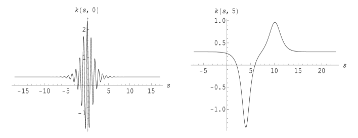
Figure 1. Left: Breather solution (2.52) with $\alpha=7,\beta=1,b=0.3$ at $t=0$.Β  Right: Double Pole solution (2.53) with $\beta=1,\leavevmode\nobreak\ b=0.3$ at $t=5$.

a

3. Summary and remarks

In this paper we have obtained the breather solution of the focusing mKdV equation with nonvanishing boundary conditions at infinity (2.52) by using the inverse scattering method for potentials that are not trivial at infinity as it was devised by T.Kawata and H.Inoue in [8]. As far as we know, it has not been reported before a systematic work on the obtention of this kind of breather solutions of mKdV under the ISM. These solutions play an important role in the construction of closed curves with localized perturbations, which evolve under the mKdV flow of curves (see [2]). We have also generalized the Double Pole solution found by M.Wadati et al. [11] to the case when it takes non trivial values $b$ at infinity. We have shown that even in this generalization, the distance between humps grows proportionally to $\log(t)$, as the formula (2.55) shows. Moreover, the associated closed curve to this (Double Pole curvature) solution is a closed curve with two loops. These two loops enclose asymptotically the same area, they point in- and outward respectively the closed curve, travel in the same direction and the distance between them grows slowly (proportionally to $\log(t)$ as $t$ goes to $\infty$) (see [2]). We think that the asymptotic property (2.55) could be useful to check the accuracy of numerical methods (e.g. difference and pseudo spectral methods) for $t$ big enough, as it was shown in [3] when $b=0$.

Finally we would like to remark that it is possible to obtain new solutions of the defocusing mKdV equation

βˆ‚kβˆ‚t+βˆ‚kβˆ‚s3βˆ’6​k2β€‹βˆ‚kβˆ‚s=0,(s,t)βˆˆβ„Γ—β„.formulae-sequenceπ‘˜π‘‘π‘˜superscript𝑠36superscriptπ‘˜2π‘˜π‘ 0𝑠𝑑ℝℝ\frac{\partial k}{\partial t}+\frac{\partial k}{\partial s^{3}}-6k^{2}\frac{\partial k}{\partial s}=0,\leavevmode\nobreak\ \leavevmode\nobreak\ (s,t)\in\mathbb{R}\times\mathbb{R}. (3.1)

from the focusing mKdV breather solutions in (2.52) with a special choice of their free parameters $b,\beta,\alpha$. With this goal in mind, we make the following changes of parameters in (2.52): $b\leavevmode\nobreak\ \text{becomes}\leavevmode\nobreak\ ib,\leavevmode\nobreak\ \leavevmode\nobreak\ \beta\leavevmode\nobreak\ \text{becomes}\leavevmode\nobreak\ -\beta$ and $\alpha\leavevmode\nobreak\ \text{becomes}\leavevmode\nobreak\ i\alpha$. Then, we get a new purely complex solution i​k~​(s,t)𝑖~π‘˜π‘ π‘‘i\tilde{k}(s,t) of the focusing mKdV equation (1.1). Hence k~​(s,t)~π‘˜π‘ π‘‘\tilde{k}(s,t) is a real and regular two soliton solution of the defocusing mKdV equation (3.1) with nonvanishing boundary value $b$ at infinity. With other selections of the parameters, $b,\beta,\alpha$ and with the same procedure, we obtain different complex and regular or singular (depending on the selected parameters) solutions of the equation (3.1) with nonvanishing boundary value $b$ at infinity.

References

  • [1] M.J. Ablowitz, D.J. Kaup, A.C. NewelΒ andΒ  H. Segur. Method for solving the sine-Gordon equation. Phys.Rev.Letters 30, 1262–1264 (1973).
  • [2] M.A. Alejo, Geometric breathers of the mKdV equation. Submitted.
  • [3] M.A. Alejo,Β C. Gorria Β andΒ  L. Vega, Discrete Conservation laws and the convergence of long time simulations of the mKdV equation. Submitted.
  • [4] T. Au-Yeung, P. C. W. Fung Β andΒ  C. Au, Modified KdV solitons with non-zero vacuum parameter obtainable from the ZS-AKNS inverse method, J. Phys. A: Math. Gen. 17 (1984) 1425–1436.
  • [5] K.W. ChowΒ andΒ  D.W. Lai, Coalescence of Ripplons, Breathers, Dromions and Dark Solitons, J.Phys.Soc.Japan, 70, n 3, (2001), 666–677.
  • [6] R.E. GoldsteinΒ andΒ D.M. Petrich, The Korteweg-de Vries Hierarchy as Dynamics of Closed Curves in the Plane, Phys.Rev.Lett., 67, n 23, (1991), 3203–3206.
  • [7] R. Grimshaw, A. Slunyaev, E. Pelinovsky, Generation of solitons and breathers in the extended Korteweg-de Vries equation with positive cubic nonlinearity. Chaos 20 (2010), no. 1, 01310201–01310210.
  • [8] H. InoueΒ andΒ T. Kawata, Inverse Scattering Method for the Nonlinear Evolutions under Nonvanishing Conditions, J.Phys.Soc.Japan,44 n 5(1978),1722–1729.
  • [9] C. Kenig, G. PonceΒ andΒ L. Vega, On the Ill-posedness of some Canonical Dispersive Equations, Duke Mathematical Journal, 106, n 3, (2001) 617-633.
  • [10] G.L. Lamb, Elements of Soliton Theory, Pure Appl.Math., Wiley, New York, 1980.
  • [11] K. OhkumaΒ andΒ M. Wadati, Multiple-Pole Solutions of the Modified Korteweg-de Vries Equation, J.Phys.Soc.Japan, 51, n 6, (1982), 2029-2035.
  • [12] D. Pelinovsky, R. Grimshaw, Structural transformation of eigenvalues for a perturbed algebraic soliton potential. Phys. Lett. A 229 (1997), no. 3, 165-172.
  • [13] M. Wadati, The modified Korteweg-de Vries Equation, J.Phys.Soc.Japan, 34, n 5, (1973), 1289-1296.