Robust classification of salient links in complex networks

Abstract

Complex networks in natural, social, and technological systems generically exhibit an abundance of rich information. Extracting meaningful structural features from data is one of the most challenging tasks in network theory. Many methods and concepts have been proposed to address this problem such as centrality statistics, motifs, community clusters, and backbones, but such schemes typically rely on external and arbitrary parameters. It is unknown whether generic networks permit the classification of elements without external intervention. Here we show that link salience is a robust approach to classifying network elements based on a consensus estimate of all nodes. A wide range of empirical networks exhibit a natural, network-implicit classification of links into qualitatively distinct groups, and the salient skeletons have generic statistical properties. Salience also predicts essential features of contagion phenomena on networks, and points towards a better understanding of universal features in empirical networks that are masked by their complexity.

I Introduction

Many systems in physics, biology, social science, economics, and technology are best modeled as a collection of discrete elements that interact through an intricate, complex set of connections. Complex network theory, a marriage of ideas and methods from statistical physics and graph theory, has become one of the most successful frameworks for studying these systems Newman2003 ; Strogatz2001 ; Albert2002 ; Boccaletti2006 ; Vespignani2009 ; Thiemann2010 ; Brockmann:2010vd and has led to major advances in our understanding of transportation Barrat2004a ; Guimera2005a ; Brockmann2006 ; woolley2011 , ecological systems Allesina2008 ; Camacho2002 , social and communication networks Lazer2009 , and metabolic and gene regulatory pathways in living cells Jeong2000 ; Almaas2004 ; Barabasi:2004cy .

One of the challenges in complex network research is the identification of essential structural features that are typically masked by the network’s topological complexity Newman2003 ; Ravasz2003 ; Thiemann2010 ; Alon2007 ; Newman2004a . Reducing a large-scale network to its core components, filtering redundant information, and extracting essential components are not only critical for efficient network data management. More importantly, these methods are often required to better understand evolutionary and dynamical processes on networks and to identify universal principles of network design or growth. In this context, the notion of centrality measures according to which nodes or links can be ranked is fundamental and epitomized by the node degree $k$, the number of directly connected neighbors of a node. Many systems, ranging from human sexual contacts Liljeros2001 to computer networks Kleinberg2001 , are characterized by a power-law degree distribution $p(k)\sim k^{-(1+\beta)}$ with an exponent $0<\beta\leq 2$. These networks are scale-free Barabasi1999 , meaning the majority of nodes are weakly connected and dominated by a few strongly connected nodes, known as hubs. Although a variety of networks can be understood in terms of their topological connectivity (the set of nodes and links), a number of systems are better captured by weighted networks in which links carry weights $w$ that quantify their strengths Barrat2004a ; Newman2004 . An important class of networks exhibit both a scale-free degree distribution and broadly distributed weights which in some cases follow a power-law $p(w)\sim w^{-(1+\alpha)}$, with $1<\alpha\leq 3$ Colizza2006 ; Brockmann:2008p1135 ; Hufnagel:2004kt . In addition to hubs, these networks thus possess highways. Several representative networks of this class are depicted in Figure 1. Understanding the essential underlying structures in these networks is particularly challenging because of the mix of link and node heterogeneity.

	Full network											Salient skeleton
Network	$N$	$\rho$		$\left<k\right>$		$\text{CV}(k)$		$\text{CV}(w)$		$r$		% links		$\beta_{\text{HSS}}$		$r_{\text{HSS}}$
Cash flow	3,106	0.	076	237.	0	1.	08	7.	72	-0.	137	0.	84	1.	10	-0.	255
Air traffic	1,227	0.	024	29.	4	1.	30	2.	25	-0.	063	6.	76	1.	60	-0.	302
Shipping	951	0.	057	54.	3	1.	22	7.	27	-0.	143	3.	66	1.	37	-0.	169
Commuting	3,141	0.	027	82.	3	1.	04	20.	80	0.	017	2.	44	2.	50	-0.	0813
Neural	297	0.	049	14.	5	0.	87	1.	42	-0.	163	13.	5	1.	61	-0.	308
Metabolic	311	0.	027	8.	4	1.	80	8.	56	-0.	253	23.	1	1.	90	-0.	381
Food web	125	0.	246	30.	5	0.	47	11.	80	-0.	117	6.	5	1.	71	-0.	437
Inter-industry	128	1.	000	127.	0	0.	00	1.	70	-0.	022	1.	08	1.	58	-0.	283
World trade	188	0.	446	83.	4	0.	65	8.	85	-0.	602	2.	39	1.	71	-0.	355
Collaboration	5,835	8.	12$\times 10^{-4}$	4.	7	0.	96	1.	21	0.	185	41.	9	1.	22	-0.	242

Table 1: Statistical features of the full empirical networks and their high-salience skeletons. Statistics for the full networks include number of nodes $N$, link density $\rho=2L/(N^{2}-N)$ (where $L$ is the number of links), mean node degree $\left\langle k\right\rangle$, coefficients of variation of node degree $\text{CV}(k)$ and link weight $\text{CV}(w)$, and the assortativity coefficient $r$ Newman2002 . For the high-salience skeletons, the first column lists the percentage of links from the full network that are also in the HSS, an estimate of the scaling exponent Clauset2009 $\beta_{\text{HSS}}$ and the assortativity coefficient $r_{\text{{HSS}}}$. Further information on network statistics are provided in Supplementary Table S1.

Although classifications of network elements according to degree, weight, or other centrality measures have been employed in many contexts Borgatti2006 ; Guimera2005a ; Wu2006 ; Wang2008 , this approach comes with several drawbacks. The qualitative concepts of hubs and highways suggest a clear-cut, network-intrinsic categorization of elements. However, these centrality measures are typically distributed continuously and generally do not provide a straightforward separation of elements into qualitatively distinct groups. At what precise degree does a node become a hub? At what strength does a link become a highway? Despite significant advances, current state-of-the-art methods rely on system-specific thresholds, comparisons to null models, or imposed topological constraints Tumminello2005 ; Serrano2009a ; Thiemann2010 ; woolley2011 ; Radicchi2011 . Whether generic heterogeneous networks provide a way to intrinsically segregate elements into qualitatively distinct groups remains an open question. In addition to this fundamental question, centrality thresholding is particularly problematic in heterogeneous networks since key properties of reduced networks can sensitively depend on the chosen threshold.

Here we address these problems by introducing the concept of link salience. The approach is based on an ensemble of node-specific perspectives of the network, and quantifies the extent to which a consensus among nodes exists regarding the importance of a link. We show that salience is fundamentally different from link betweenness centrality and that it successfully classifies links into distinct groups without external parameters or thresholds. Based on this classification we introduce the high-salience skeleton (HSS) of a network and compute this structure for a variety of networks from transportation, biology, sociology, and economics. We show that despite major differences between representative networks, the skeletons of all networks exhibit similar statistical and topological properties and significantly differ from alternative backbone structures such as minimal spanning trees. Analyzing traditional random network models we demonstrate that neither broad weight nor degree distributions alone are sufficient to produce the patterns observed in real networks. Furthermore, we provide evidence that the emergence of distinct link classes is the result of the interplay of broadly-distributed node degrees and link weights. We demonstrate how a static and deterministic analysis of a network based on link salience can successfully predict the behavior of dynamical processes. We conclude that the large class of networks that exhibit broad weight and degree distributions may evolve according to fundamentally similar rules that give rise to similar core structures.

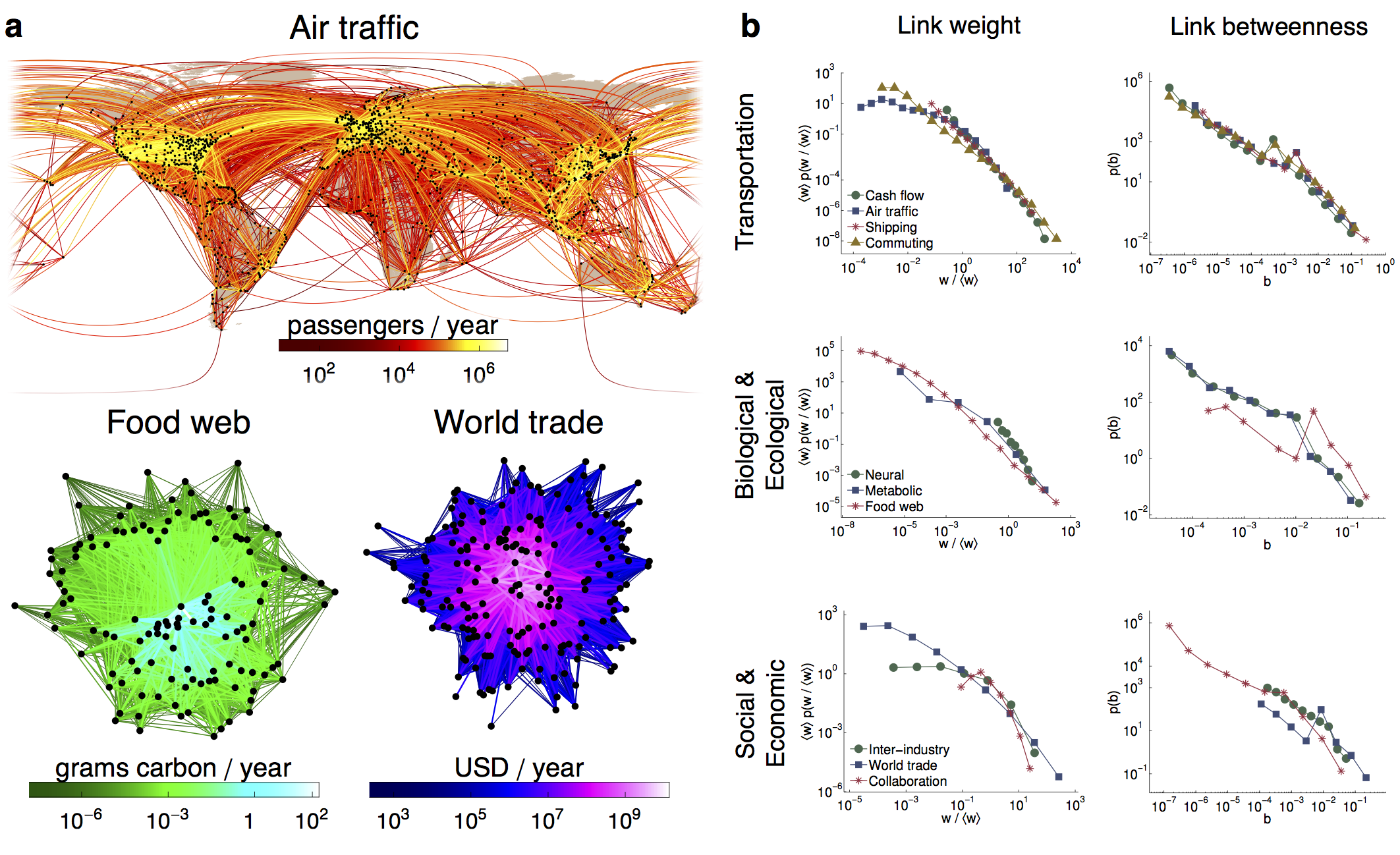
Figure 1: Generic statistical properties of heterogeneous complex networks. (a) Geographic representation of the worldwide air traffic network (top), black dots represent airports, links represent passenger flux between them, link weights $w_{ij}$ are color encoded from dark (weak) to white (strong). Networks on the lower left and right represent the Florida bay food web and the world trade network, respectively. Nodes in the food web are species and links represent the exchange of biomass; in the trade network nodes are countries and links quantify exchange in assets measured in United States dollars (USD). (b) Relative frequencies $f(w)=\left\langle w\right\rangle p(w/\left\langle w\right\rangle)$ and $p(b)$ of link weights $w$ and link betweenness $b$ of representative transportation, biological, ecological, social, and economic networks. Link weights are normalized by the mean weight $\left\langle w\right\rangle$. Details on each network are provided in Methods. In all networks link weights and betweenness are distributed across many orders of magnitude, and both statistics exhibit heavy tails. The substantial variability in these quantities is also reflected in their coefficient of variation (see Table 1).

II Results

II.1 Link salience

Weighted networks like those depicted in Figure 1 can be represented by a symmetric, weighted $N\times N$ matrix $W$ where $N$ is the number of nodes. Elements $w_{ij}\geq 0$ quantify the coupling strength between nodes $i$ and $j$. Depending on the context, $w_{ij}$ might reflect the passenger flux between locations in transportation networks, the synaptic strength between neurons in a neural network, the value of assets exchanged between firms in a trade network, or the contact rate between individuals in a social network.

Our analysis is based on the concept of effective proximity $d_{ij}$ defined by the reciprocal coupling strength $d_{ij}=1/w_{ij}$. Effective proximity captures the intuitive notion that strongly (weakly) coupled nodes are close to (distant from) each other Caldarelli2007 . It also provides one way to define the length of a path $\mathcal{P}$ that connects two terminal nodes ($n_{1},n_{K}$) and consists of $K-1$ legs via a sequence of intermediate nodes $n_{i}$, and connections $w_{n_{i}n_{i+1}}>0$. The shortest path minimizes the total effective distance $l=\sum_{i=1}^{K-1}d_{n_{i}n_{i+1}}$ and can be interpreted as the most efficient route between its terminal nodes Dijkstra1959a ; Newman2010 ; this definition of shortest path is used throughout this paper. In networks with homogeneous weights, shortest paths are typically degenerate, and many different shortest paths coexist for a given pair of terminal nodes. In heterogeneous networks with real-valued weights shortest paths are typically unique. For a fixed reference node $r$, the collection of shortest paths to all other nodes defines the shortest-path tree (SPT) $T(r)$ which summarizes the most effective routes from the reference node $r$ to the rest of the network. $T(r)$ is conveniently represented by a symmetric $N\times N$ matrix with elements $t_{ij}(r)=1$ if the link $(i,j)$ is part of at least one of the shortest paths and $t_{ij}(r)=0$ if it is not.

The central idea of our approach is based on the notion of the average shortest-path tree as illustrated in Figure 2a. We define the salience $S$ of a network as

$$S=\left\langle T\right\rangle=\frac{1}{N}\sum_{k}T(k)$$ (1)

so that $S$ is a linear superposition of all SPTs. $S$ can be calculated efficiently using a variant of a standard algorithm (see Supplementary Methods). According to this definition the element $0\leq s_{ij}\leq 1$ of the matrix $S$ quantifies the fraction of SPTs the link $(i,j)$ participates in. Since $T(r)$ reflects the set of most efficient paths to the rest of the network from the perspective of the reference node, $s_{ij}$ is a consensus variable defined by the ensemble of root nodes. If $s_{ij}=1$ then link $(i,j)$ is essential for all reference nodes, if $s_{ij}=0$ the link plays no role and if, say, $s_{ij}=1/2$ then link $(i,j)$ is important for only half the root nodes. Note that although $S$ is defined as an average across the set of shortest-path trees, it is itself not necessarily a tree and is typically different from known structures such as minimal spanning trees (see Supplementary Figure S1, Supplementary Table S3 and Supplementary Methods).

II.2 Robust classification of links

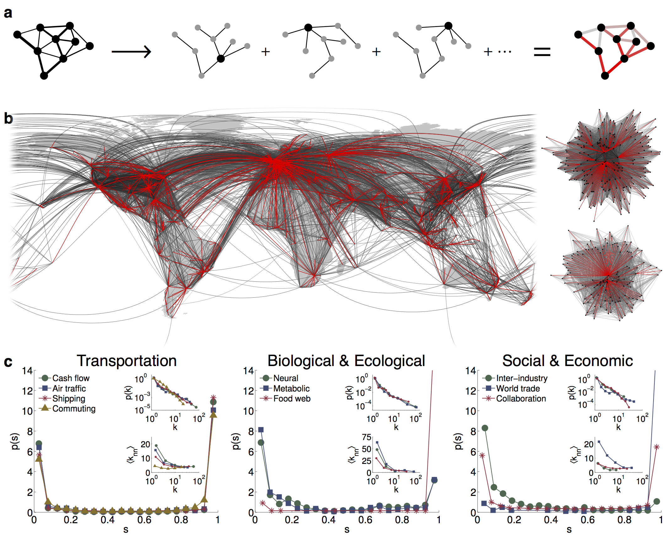
Figure 2: Computation of link salience and properties of the high-salience skeleton. (a) For each reference node $r$ in the weighted network on the left the shortest-path tree $T(r)$ is computed. The superposition of all trees according to Equation (1) assigns a value $s_{ij}$ to each link in the original network. Salience values are shown on the right with link color: red is high salience and grey is low. (b) The collection of high salience links (red) for the networks shown in Figure 1. The full networks are shown in grey. (c) The relative frequency $p(s)$ of non-zero salience values $s$. The distribution $p(s)$ is bimodal in all networks under consideration. This key feature of bimodality of $p(s)$ provides a plausible, parameter-insensitive classification of links, salient ($s\approx 1$) vs. non-salient ($s\approx 0$), and implies that nodes in these networks typically agree whether a link is essential or not. The high-salience skeleton (HSS) is defined as the collection of links that accumulate near $s\approx 1$. Upper and lower insets depict, respectively, the degree distribution $p(k)$ of the HSSs and mean next-neighbor degree $\left\langle k_{nn}|k\right\rangle$ as a function of node degree $k$. The HSS degree distribution is typically scale-free (see Supplementary Figure S2) and the skeletons are typically strongly disassortative. Note that although they may be, and often are, divided into multiple components, the largest connected component of the skeleton typically dominates. This connectedness is not imposed, but is an emergent property of salience. (See Supplementary Table S2).

The most important and surprising feature of link salience is depicted in Figure 2c. For the representative set of networks, we find that the distribution $p(s)$ of link salience exhibits a characteristic bimodal shape on the unit interval. The networks’ links naturally accumulate at the range boundaries with a vanishing fraction at intermediate values. Salience thus successfully classifies network links into two groups: salient ($s\approx 1$) or non-salient ($s\approx 0$), and the large majority of nodes agree on the importance of a given link. Since essentially no links fall into the intermediate regime, the resulting classification is insensitive to an imposed threshold, and is an intrinsic and emergent network property characteristic of a variety of strongly heterogeneous networks. This is fundamentally different from common link centrality measures such as weight or betweenness that possess broad distributions (see Fig. 1b), and which require external and often arbitrary threshold parameters for meaningful classifications Serrano2009a ; Radicchi2011 .

The salience as defined by Eq. 1 permits an intuitive definition of a network’s skeleton as a structure which incorporates the collection of links that accumulate at $s\approx 1$. Figure 2b depicts the skeleton for the networks of Figure 1a. For all networks considered, only a small fraction of links are part of the high-salience skeleton (6.76% for the air traffic network, 6.5% for the food web, and 2.39% for the world trade network), and the topological properties of these skeletons are remarkably generic. Note that technically a separation of links into groups according to salience requires the definition of a threshold (e.g. we chose the center of the salience range for convenience). The important feature is that the resulting groups are robust against changes in the value, since almost no links fall into intermediate ranges. Consequently the point of separation is almost arbitrary, yield almost identical skeletons for threshold ranges of $80\%$ of the entire range. One of the common features of these skeletons is their strong disassortativity, irrespective of the assortativity properties of the corresponding original network (see Table 1). Furthermore, all skeletons exhibit a scale-free degree distribution

$$p_{\text{HSS}}(k)\sim k^{-(1+\beta_{\text{HSS}})}$$ (2)

with exponents $1.1\leq\beta_{\text{HSS}}\leq 2.5$ (see Table 1 and Supplementary Figure S2). Since only links with $s\approx 1$ are present in the HSS, the degree of a node in the skeleton can be interpreted as the total salience of the node. The collapse onto a common scale-free topology is particularly striking since the original networks range from quasi-planar topologies with small local connectivity (the commuter network) to completely connected networks (worldwide trade). Note that the lowest exponent (weakest tail) is observed for the commuter network, since in a quasi-planar network the maximum number of salient connections is limited by the comparatively small degree of the original network. The scale-free structure of the HSS consequently suggests that networks that possess very different statistical and topological properties and that have evolved in a variety of contexts seem to self-organize into structures that possess a robust, disassortative backbone, despite their typical link redundancy.

Although these properties of link salience are encouraging and suggest novel opportunities for filtering links in complex weighted networks, for understanding hidden core sub-structures, and suggest a new mechanism for defining a network’s skeleton, a number of questions need to be addressed and clarified in order for the approach to be viable. First, a possible criticism concerns the definition of salience from shortest-path trees which suggests that $s_{ij}$ can be trivially obtained from link betweenness $b_{ij}$, for example by means of a non-linear transform. Secondly, a bimodal $p(s)$ may be a trivial consequence of broad weight distributions, if for instance large weights are typically those with $s\approx 1$. Finally, the observed bimodal shape of $p(s)$ could be a property of any non-trivial network topology such as simple random weighted networks. In the following we will address each of these concerns.

II.3 Salience and betweenness

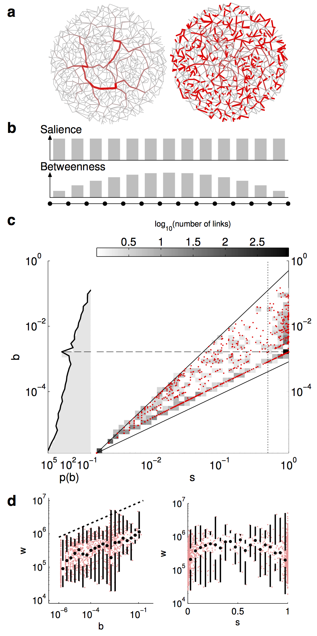
Figure 3: Salience and betweenness capture different aspects of centrality.  (a) A schematic planar network in which the color of links quantifies betweenness $b$ (left) and salience $s$ (right). High-betweenness links tend to be located near the barycenter of the network Barthelemy2011 , whereas high-salience links are distributed evenly throughout the network.  (b) A simple linear chain shows the reason for this effect. A link in the center serves as a shortest-path bridge between all pairs of nodes, and so has the highest betweenness. But since all shortest-path trees are identical, all links have identical salience.  (c) A scatter plot (red dots) of link salience $s$ versus link betweenness $b$ for the air traffic network (point density is quantified in grey). The vertical dotted line marks $s=1/2$ and the solid curves represent the theoretical bounds of Equation (3). The projected density $p(b)$ is shown on the left. The lack of any clear correlation in the scatter plot is typical of all networks in Figure 1. (See Supplementary Figure S3 for additional correlograms.)  (d) Scatter plots (in light red) of betweenness $b$ (left) and salience $s$ (right) versus link weight $w$ in the air traffic network. The bottom and top of the lower whiskers, the dot, and the bottom and top of the upper whiskers correspond to the 0, 25, 50, 75, and 100th percentiles, respectively. The dashed line indicates a scaling relationship $w\sim b^{\gamma}$ with $\gamma\approx 0.2$. Although the network exhibits a positive correlation between link weight and link betweenness, the high-salience skeleton incorporates links with weights spanning the entire range of observed values; no clear correlation of weight with salience exists. These properties are observed in the other networks as well.

The betweenness $b_{ij}$ of a link $(i,j)$ is the fraction of all $\sim N^{2}$ shortest paths that pass though the link, whereas the salience $s_{ij}$ is the fraction of $N$ shortest-path trees $T(r)$ the link is part of. Despite the apparent similarity between these two definitions, both quantities capture very different qualities of links, as illustrated in Figure 3. Betweenness is a centrality measure in the traditional sense Freeman1977 , and is affected by the topological position of a link. Networks often exhibit a core-periphery structure Holme2005 and the betweenness measure assigns greater weight to links that are closer to the barycenter of the network Barthelemy2011 . Salience, on the other hand, is insensitive to a link’s position, acting as a uniform filter. This is illustrated schematically in the random planar network of Figure 3a. High betweenness links tend to be located in the center of the planar disk, whereas high salience links are distributed uniformly. A given shortest path is more likely to cross the center of the disk, whereas the links of a shortest-path tree are uniformly distributed, as they have to span the full network by definition. A detailed mathematical comparison of betweenness and salience is provided in the Methods. Figure 3c depicts the typical relation of betweenness and salience in a correlogram for the worldwide air traffic network. The data cloud is broadly distributed within the range of possible values given by the inequalities (see Supplementary Methods)

$$s/N\leq b\leq s^{2}/2.$$ (3)

Within these bounds no functional relationship between $b$ and $s$ exists. Given a link’s betweenness $b$ one generally cannot predict its salience and vice versa. In particular, high-salience links ($s\approx 1$) possess betweenness values ranging over many scales. The spread of data points within the theoretical bounds is typical for all the networks considered (see Supplementary Figure S3). Links tend to collect at the right-hand edge, corresponding to the upper peak in salience, and in particular at the lower right corner of the wedge-shaped region, corresponding to the heretofore-unexplained peak in betweenness exhibited by several of the networks (cf. Figure 1 and the dashed line in Figure 3b). These edges have maximal salience (all nodes agree on their importance) but the smallest betweenness possible given this restriction (they are not well-represented in the set of shortest paths). Such edges are the spokes in the hub-and-spoke structure: they connect a single node to the rest of the network, but are used by no others, and they are an essential piece of the high-salience skeleton, since severing them removes some node’s best link to the main body of the network. The presence of such links in the high-salience skeleton explains why the weight values of $s\approx 1$ edges span such a wide range, since a link may have relatively low weight and yet be some node’s most important connection.

Figure 3d tests the hypothesis that strong link weights may yield strong values for salience. We observe that link betweenness is positively correlated with link weight and roughly follows a scaling relation $w\sim b^{\gamma}$ with $\gamma\approx 0.2$, in agreement with previous work on node centrality DallAsta2006 . This is not surprising since high-weight links are by definition shorter and tend to attract shortest paths. In contrast, link weights exhibit no systematic dependence on salience, and in particular large weights do not generally imply large salience. In fact, for fixed link salience the distribution of weights is broad with approximately the same median. Consequently, salience can be considered an independent centrality dimension that measures different features than correlated centrality measures such as weight and betweenness.

II.4 Origin of bimodal salience

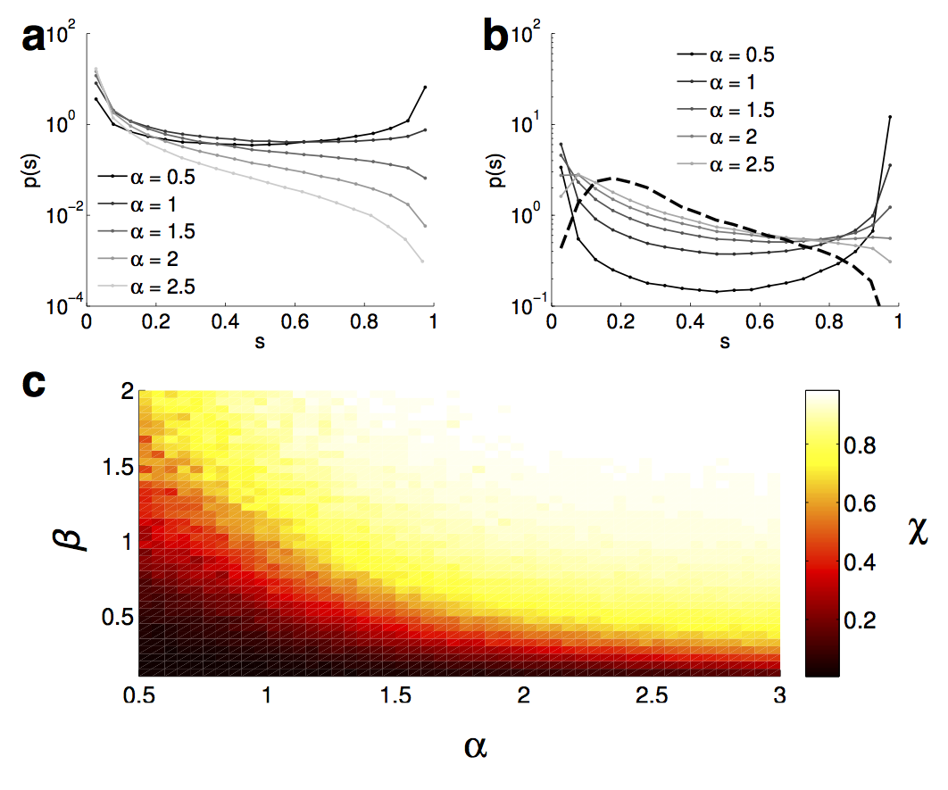
Figure 4: Salience in random networks.  (a) Salience distributions $p(s)$ in fully connected networks with 1,000 nodes and weights assigned using a power law $p(w)\sim w^{-(1+\alpha)}$ for various tail exponents $\alpha$. Complete networks serve as models of systems with all-to-all interactions, such as the inter-industry trade network. Only for unrealistically broad weight distributions ($\alpha\lesssim 1$) does $p(s)$ exhibit a bimodal character. If $\alpha>1$ bimodality is absent.  (b) Salience distributions in preferential attachment networks (1,000 nodes) Barabasi1999 with degree distribution $p(k)\sim k^{-3}$ and uniform weights do not exhibit bimodal salience (heavy dashed line). If however the power-law weight distribution is superimposed on the preferential attachment topology, bimodal salience emerges for realistic values of $\alpha$.  (c) For the range of tail exponents $\alpha$ and $\beta$ the color code quantifies the magnitude $\chi$ of bimodality in the salience distribution $p_{\alpha.\beta}(s)$ of a network with a scale-free degree distribution with exponent $\beta$ (constructed using the configuration model Boccaletti2006 ) and a scale-free weight distribution with exponent $\alpha$. Small values of $\chi$ correspond to a bimodal $p_{\alpha,\beta}(s)$. The bimodality measure $\chi$ was computed using Kolmogorov-Smirnov distance between $p_{\alpha,\beta}(s)$ for $s>0$ and the idealized reference distribution $q(s)=\delta(s-1)$.

All the networks we consider feature broad link weight distributions $p(w)$ (see Figure 1b), some of which can be reasonably modeled by power laws $p(w)\sim w^{-(\alpha+1)}$ with exponents for many empirical data sets typically in the range $1<\alpha<3$ Clauset2009 (smaller $\alpha$ corresponds to broader $p(w)$). Although it may seem plausible that strong links in the tail of these distributions dominate the structure of shortest-path trees and thus cause the characteristic bimodal distribution of link salience, evidence against this hypothesis is already apparent in Fig 3d: links with high salience exhibit weights across many scales, and in particular low-weight links may possess high salience. Further evidence is provided in Figure 4a, which depicts the salience distribution for fully connected networks for a sequence of tail parameters $\alpha$. For values of $\alpha$ in the range observed in real networks, $p(s)$ is peaked near $s=0$ and decreases with increasing $s$. A bimodal distribution of $s$ only emerges when $\alpha$ is unrealistically small ($\alpha<1$), and is much less pronounced than in real networks (cf. Figure 2). We conclude that broad, scale-free weight distributions $p(w)$ alone are insufficient to cause the natural, bimodal distribution $p(s)$ observed in real networks.

Another potential source of the observed bimodality in $p(s)$ is the topological heterogeneity of a scale-free degree distribution $p(k)\sim k^{-(1+\beta)}$ with $0<\beta<2$ Barabasi1999 ; Kleinberg2001 ; Guimera2007 . Figure 4b provides evidence that also a scale-free topology alone does not yield the characteristic bimodal salience distribution. In fact, the generic preferential attachment network Barabasi1999 ($\beta=2$) with uniform weights exhibits a distribution of salience that is almost the complement of the observed pattern with mostly intermediate values of link salience. The presence of hubs implies that any shortest paths seeking out a node in a hub’s region will most likely route through that hub, and links emanating from this hub are more likely to appear in many shortest-path trees. However, the hub-and-spoke structure of a preferential attachment network is only approximate; nodes that are at the end of a spoke are still likely to have random links to other areas of the network. For this reason, it is not typical in the uniform-weight preferential attachment network to find links that appear in nearly all shortest-path trees.

However, the observed bimodal distribution $p(s)$ can be generated in random networks by a combination of weight and degree variability, a property characteristic of the class of networks discussed here. Figure 4b also depicts $p(s)$ for preferential attachment networks that possess a scale-free distribution of both degree $k$ and weight $w$. As the weight distribution becomes broader (decreasing $\alpha$), and even in the absence of explicit degree-weight correlations, we see the emergence of bimodality in the salience distribution in these networks. Topological hubs are more likely to have extremely high-weight links simply because they have more links. Even when there is a topologically short path terminating at a spoke node that does not pass through the corresponding hub, it is less likely to be the shortest weighted path. Extreme weights amplify the effects of hubs by drawing more shortest paths through them. Moreover, Figure 4c demonstrates that the emergence of bimodal salience does depend on the interplay between degree and weight distributions: the broader the degree distribution, the narrower the required weight distribution.

All of these results support the conclusion that a bimodal salience distribution is characteristic of networks with strong heterogeneity in both topology and interaction strength, but that unweighted networks do not exhibit this property.

II.5 Applications to network dynamical systems

Figure 5: Salience predicts infection pathways in stochastic epidemic models. The scatter plots show the directed salience $s_{d}$ against the normalized frequency of appearance in infection pathways $h$ for each link in an ensemble of 100 networks, averaged over 1,000 epidemic realizations for each member of the ensemble. As in Figure 3, the plots are divided horizontally into bins, with the heavy black lines indicating quartiles within each bin. Insets show link betweenness $b$ versus $h$, and correlation coefficients are listed in Table 3.  top, Weights distributed narrowly and uniformly around a constant $w_{0}$.  bottom, Weights distributed according to $p(w)\sim w^{-(1+\alpha)}$ with $\alpha=2$.

The relevance of link salience to dynamical processes that evolve on networks is an important issue, and one area of particular interest in network research is contagion phenomena. In this context, individuals in a population are represented by nodes, and interaction propensities between pairs of nodes by a weighted network. Contagion phenomena are modeled by transmissions between nodes along the links of the network, where the likelihood of transmission is quantified by the link weights. The central question in this class of models is how the topological properties of the network shape the dynamics of the process. Link salience can also provide useful information about the behavior of such a dynamical system. To illustrate this, we consider a simple stochastic SI epidemic model. At any given point in time, an infected node $i$ can transmit a disease to susceptible nodes at a rate determined by the link weight $w_{ji}$. The details of the model are provided in the Methods. We consider an epidemic on a planar disk network similar to that shown in Figure 3a. A single node is chosen at random for the outbreak location. At every step of the process each infected node randomly selects a neighbor to infect with probability proportional to the link weight; eventually the entire network is infected. By keeping track of which links were used in the infection process one obtains the infection hierarchy $H$, a directed tree structure that represents the epidemic pathway through the network. Since the process is stochastic, each realization of the process generates a different infection hierarchy. For different initial outbreak nodes and realizations of the process we calculate an infection frequency $h$ for each link: The number of times that link is used in the infection process, normalized by the number of realizations. The question is, how successfully can link salience, a topological quantity, predict infection frequency $h$, a dynamic quantity. Figure 5 shows the results for the two different link weight scenarios described in the Methods. The top panel shows networks with link weights narrowly and uniformly distributed around a constant value $w_{0}$; in the bottom panel link weights are broadly distributed according to a power law. In both cases, link salience is highly correlated with the frequency of a link’s appearance in infection hierarchies $h$, while alternative link centrality measures such as weight and betweenness are not (see Figure 5 insets and SI). The link salience on average gives a much more accurate prediction of the virulence of a link than other available measures of centrality, suggesting that this type of completely deterministic, static analysis could nonetheless play an important role in considering how best to slow spreading processes in real networks.

III Discussion

As much recent work in network theory has shown Serrano2009a ; Tumminello2005 ; Newman2004a ; Alon2007 , there is tremendous potential for extracting heretofore hidden information from the complex interactions between the elements of a system. However, until now these methods have relied on externally imposed parameters or null models. Here we have shown that typical empirical networks taken from a variety of fields do in fact permit the robust classification of links according to the node-consensus procedure we introduce, and that this leads naturally to the definition of a high-salience skeleton in these networks. Because vanishingly few links in empirical networks have intermediate values of salience, the identification of the skeleton is insensitive to a salience threshold; indeed, if a tunable filtering procedure is desired other methods may be more appropriate. Not all networks possess a skeleton; simple unweighted models have a shortest-path structure spread throughout the links. However, the presence of a skeleton is a generic feature of many heterogeneously weighted, empirical networks. We suggest that the likely cause in real networks is a hub-and-spoke topological structure along with a broad weight distribution, which amplifies the tendency of hubs to capture shortest paths.

We believe that the concept of salience and the high-salience skeleton will become a vital component in understanding networks of the type discussed here and the development of network-based dynamical models. The simple SI model we investigate here is only a starting point; it may be possible to leverage knowledge of a network’s high-salience skeleton to develop dynamical models that do not require simulation on (or even knowledge of) the full network. The generic bimodal salience distribution in this context also implies that in contagion phenomena only a small subset of links might typically be active even if the process is stochastic. Those links, however, are almost certainly active irrespective of the outbreak location and the stochasticity of the process, which implies that in this regime the process becomes more predictable and the impact of stochasticity is decreased. This effect may shed a new light on the impact of stochastic factors in disease dynamical processes that evolve in strongly heterogeneous networks.

Many of the networks we considered evolved over long periods of time subject to external constraints and unknown optimization principles. The discovery that pronounced weight and degree heterogeneity, which are defining properties of the investigated networks, go hand in hand with generic properties in their underlying skeleton indicate that looking for common evolution principles could be another promising direction of further research.

IV Methods

IV.1 Network data sources

Network	Nodes	Link units
Cash flow	Counties, continental United States	Number of bills/time
Air traffic	Airports, worldwide	Number of passengers/time
Shipping	Ports, worldwide	Number of cargo ships/time
Commuting	Counties, continental United States	Number of commuters/times
Neural	Neurons, C. elegans	Number of synapses and gap junctions
Metabolic	Metabolites, E. coli	Effective kinetic reaction rate
Food web	Species, Florida Bay food web	Exchanged biomass/time
Inter-industry	Industrial sectors, United States	Average input required for fixed output (USD)
World trade	Countries	Average value of traded assets/time (USD)
Collaboration	Scientists	Number of co-authored papers

Table 2: Definition of nodes and links in empirical networks. The entities represented by nodes, as well as the units measured by link weight, are listed for every network.

Table 2 gives a brief definition of each network we examine here, and below we provide a summary of the networks along with data sources and references.

The Cash flow network was constructed from data collected through the Where’s George bill-tracking website (http://www.wheresgeorge.com). The nodes are the 3,106 counties in the 48 United States excluding Alaska and Hawaii, and the links measure the number of bills passing between pairs of counties per time. This network has been previously analyzed Brockmann2006 ; Thiemann2010 ; Brockmann:2008p1135 ; see in particular the supplement to Thiemann2010 for a wealth of detailed information regarding the construction and statistics of this network, as well as strong evidence for interpreting it as proxy for individual mobility. The network of cash flow is constructed from approximately 10 million individual bank notes that circulate in the United States.

The Air traffic network measures global air traffic based on flight data provided by OAG Worldwide Ltd. (http://www.oag.com) and includes all scheduled commercial flights in the world. Nodes represent airports worldwide. Link weights measures the total number of passengers traveling between a pair of networks by direct flights per year. This network is well-represented in the literature Barrat2004a ; Colizza2006 ; Guimera2005a ; Guimera2007 ; Sales-Pardo2007 ; we reduce it to 95% flux as described in Olivia1998 . Total traffic in this network amounts to approximately 3 billion passengers per year.

The Shipping network quantifies international marine freight traffic based on data provided by IHS Fairplay (http://www.ihs.com/products/maritime-information/index.aspx) which includes itineraries for 16,363 container ships. Nodes represent ports, and links measure the number of commercial cargo vessels traveling between those ports during 2007. The network is available at http://www.mathmod.icbm.de/45365.html and further discussion can be found in Kaluza2010 .

The Commuting network is based on surveys conducted by the US Census Bureau during the 2000 census, and reflects the daily commuter traffic between US counties; the data is publicly available at http://www.census.gov/population/www/cen2000/commuting/files/2KRESCO_US.zip. Nodes in this network represent the counties of the 48 states excluding Alaska and Hawaii, and links measure the number of people commuting between pairs of counties per day.

The Neural network is derived from the Caenorhabditis elegans nematode. Nodes represent neurons, and links measure the number of synapses or gap junctions connecting a pair of neurons. Experimental data is described in Ref. White1986 and analyzed in Ref. Watts1998 ; the network is available at http://www-personal.umich.edu/~mejn/netdata/.

The metabolic network measures interactions in the bacterium Escherichia coli Reed2003 ; Almaas2004 . Nodes represent metabolites and links measure effective kinetic rates of reactions a pair of metabolites participates in. We use only the largest connected component of this network.

The Food web network is a representative food web from a list of publicly available data sets of the same type (see http://vlado.fmf.uni-lj.si/pub/networks/data/bio/foodweb/foodweb.htm for networks in Pajek format, a report Ulanowicz1998 on trophic analysis of the Florida Bay food web available at http://www.cbl.umces.edu/~atlss/FBay701.html, and Refs. Serrano2009a ; Radicchi2011 ). Nodes represent species in the Florida Bay ecosystem, and links measure the consumed biomass in grams of carbon per year across a link.

In the Inter-industry network, nodes represent industrial sectors in the United States and their connections are computed from input-output tables prepared by the US Bureau of Economic Analysis available at http://www.bea.gov/industry/io_benchmark.htm. We use data from 2002, the most recent year for which measurements are available. Nodes in this network represent particular industries (for example, “tobacco production” or “cutlery and hand tool manufacturing”) and links measure an average interaction between two industries. Given two industries $x$ and $y$, input-output data measures the amount (USD) of input $x$ demands from $y$ in order to produce one dollar of output, and we take the weight of the link connecting $x$ and $y$ to be the geometric mean of the input-output demand of $x$ on $y$ and $y$ on $x$.

The World trade network is based on data prepared by the United States National Bureau of Economic Research and measures the value (in nominal thousands of USD) of goods traded between countries from 1962-2000. Nodes represent countries and links measure the value of goods traded between countries. The data and extensive documentation are available at http://cid.econ.ucdavis.edu/data/undata/undata.html. A series of papers analyzes a similar data set from a different source Radicchi2011 ; Garlaschelli2004 ; Garlaschelli2005 ; Serrano2003 .

The Collaboration network is based on co-authorship of academic papers in the high-energy physics community from 1995-1999. Nodes represent individuals and links measure the number of papers co-authored Newman2001a . The data is publicly available at http://www-personal.umich.edu/~mejn/netdata/.

IV.2 Link salience and betweenness centrality

Link salience $s$ and betweenness centrality $b$ are based on the notion of shortest paths in weighted networks. Given a weighted network defined by the weight matrix $w_{ij}$ (not necessarily symmetric) and a shortest path that originates at node $x$ and terminates at node $y$ it is convenient to define the indicator function

$$\sigma_{ij}(y,x)=\begin{cases}1&\text{if link }i\rightarrow j\text{ is on the shortest path}\\ &\quad\text{from }x\text{ to }y\\ 0&\text{otherwise}\end{cases}$$

A shortest path tree $T(x)$ rooted at node $x$ can be represented as a matrix with elements

$$T_{ij}(x)=\begin{cases}1&\text{if }\sum_{y}\sigma_{ij}(y,x)>0\\ 0&\text{otherwise},\end{cases}$$

and salience $s_{ij}$ of link $i\rightarrow j$ is given by

$$s_{ij}=\frac{1}{N}\sum_{x}T_{ij}(x)=\left\langle T_{ij}(x)\right\rangle_{V}$$ (4)

where $\left\langle\cdot\right\rangle_{V}$ denotes the average across the set of root nodes $x$.

Betweenness, on the other hand, is defined according to

$$b_{ij}=\frac{1}{N^{2}}\sum_{x,y}\sigma_{ij}(y,x)=\left\langle\sigma_{ij}(y,x)\right\rangle_{V^{2}}$$

where $\left\langle\cdot\right\rangle_{V^{2}}$ denotes the average over all $N^{2}$ pairs of terminal nodes. The relation of betweenness and salience can be made more transparent by rewriting this expectation value as a sequential average over all nodes,

$$b_{ij}=\frac{1}{N}\sum_{x}b_{ij}(x)$$

with

$$b_{ij}(x)=\frac{1}{N}\sum_{y}\sigma_{ij}(y,x)=\left\langle\sigma_{ij}(y,x)\right\rangle_{V}$$

fixing root node $x$. Thus $b_{ij}(x)$ is the conditional betweenness of link $i\rightarrow j$ if the set of shortest paths is restricted to those terminating at $x$. From this it follows that

$$b_{ij}=\left\langle\left\langle\sigma_{ij}(x,y)\right\rangle_{V}\right\rangle_{V}$$ (5)

Comparing (5) with (4) we see that the difference of salience and betweenness is equivalent to the difference in the shortest path trees $T_{ij}(x)$ and the conditional betweenness $b_{ij}(x).$ Whereas all links in the shortest path tree are weighted equally, links with non-zero conditional betweenness tend to become less central as the links become further separated from the root node $x$. Formally we can write

$$s_{ij} = \left\langle\Theta\left[\left\langle\sigma_{ij}(x,y)\right\rangle_{V}\right]\right\rangle_{V}$$

$$b_{ij} = \left\langle\left\langle\sigma_{ij}(x,y)\right\rangle_{V}\right\rangle_{V},$$ (6)

with $\Theta(x)=1$ if $x>0$ and $\Theta(x)=0$ otherwise.

IV.3 Epidemic simulations

In order to determine the relevance of link salience to contagion phenomena on networks, we investigated the correlation of link salience and the frequency at which links participate in a generic contagion process that spreads through planar, random triangular networks.

Each network consists of $N=100$ nodes distributed uniformly at random in a planar disk; the links of the network are given by the Delaunay triangulation of the nodes. The planar distance between nodes is roughly proportional to the number of links in a shortest (network) path between them. A representative example of this type of topology is shown in Figure 3a. We consider two different weight scenarios:

1. Quasi-homogeneous weights: Each link is assigned a unit weight $w$ modified by an additive, small perturbation $\xi$

   $$w=1+\xi$$

   where $\xi$ is uniformly distributed in the interval $[-0.01,0.01]$

2. Broadly distributed weights: Each link is assigned a random weight from the distribution with PDF

   $$p(w)\sim w^{-3}.$$

We simulate a stochastic Susceptible-Infected (SI) epidemic process. A single stochastic realization of the process is generated as follows: Given a network represented by the symmetric weight matrix $w_{ij}$ which quantifies the interaction strength of a pair of nodes, we define the probability $P_{ij}$ that node $j$ infects node $i$ in a fixed time interval $\Delta t$

$$P_{ij}=\gamma p_{ij}\quad i\neq j.$$

where $\gamma\ll 1/\Delta t$ is the infection rate, and $p_{ij}=w_{ij}/\sum_{i}w_{ij}$. Time proceeds in discrete steps; at each step each infected node $j$ chooses an adjacent node to infect at random with probabilities given by $P_{ij}$. If node $j$ infects a susceptible node $i$, then the link $(j,i)$ is added to the infection hierarchy $H$, which can be represented as a matrix $H_{ji}$. In the long time limit every node is infected, and $H$ is a tree structure recording the first infection paths from the outbreak location $s$ to every other node.

For a given network, we compute $R=1,000$ different epidemic realizations with random outbreak locations $s_{k}$, resulting in an ensemble of infection hierarchies $H_{mn}^{(k)}$. The key question is, how frequently does a link in the network participate in an epidemic, and we define the infection frequency of a link as

$$h_{mn}=\frac{1}{R}\sum_{k=1}^{R}H_{mn}^{(k)}$$

We compute the infection frequency for 100 random networks under each weight scenario, and Figure 5 illustrates the degree to which the directed salience $s_{mn}$ is a predictor of the dynamic quantity $h_{mn}$. The correlation of $h_{mn}$ with directed salience and the two measures of centrality we consider here, weight $w_{mn}$ and betweenness $b_{mn}$, is shown in Table 3.

Weight scenario		$s_{d}$ vs $h$		$b$ vs $h$		$w$ vs $h$
Homogeneous		$0.734$		$0.0756$		$0.005\,45$
Broad		$0.803$		$0.329$		$0.393$

Table 3: Correlation of other measures with infection frequency. The Pearson correlation coefficients of salience $s_{d}$, betweenness $b$, and weight $w$ with infection pathway frequency $h$ are shown.

Author contributions

DG, CT, and DB designed the research. DG and DB developed the theory. DG, CT and DB analysed the data. DG performed epidemic simulations. DG and DB wrote the manuscript.

Additional information

Competing financial interests:

The authors declare no competing financial interests.

References

- (1) Newman, M. E. J. The structure and function of complex networks. SIAM Review 45, 167–256 (2003).
- (2) Strogatz, S. H. Exploring complex networks. Nature 410, 268–76 (2001).
- (3) Albert, R. & Barabási, A.-L. Statistical mechanics of complex networks. Reviews of Modern Physics 74, 47–97 (2002).
- (4) Boccaletti, S., Latora, V., Moreno, Y., Chavez, M. & Hwang, D. Complex networks: Structure and dynamics. Physics Reports 424, 175–308 (2006).
- (5) Vespignani, A. Predicting the behavior of techno-social systems. Science 325, 425–8 (2009).
- (6) Thiemann, C., Theis, F., Grady, D., Brune, R. & Brockmann, D. The Structure of Borders in a Small World. PLoS ONE 5, e15422 (2010).
- (7) Brockmann, D. Following the money. Physics World 23, 31–34 (2010).
- (8) Barrat, A., Barthélemy, M., Pastor-Satorras, R. & Vespignani, A. The architecture of complex weighted networks. PNAS 101, 3747–52 (2004).
- (9) Guimerà, R., Mossa, S., Turtschi, A. & Amaral, L. A. N. The worldwide air transportation network: Anomalous centrality, community structure, and cities’ global roles. PNAS 102, 7794–9 (2005).
- (10) Brockmann, D., Hufnagel, L. & Geisel, T. The scaling laws of human travel. Nature 439, 462–465 (2006).
- (11) Woolley-Meza, O. et al. Complexity in human transportation networks: A comparative analysis of worldwide air transportation and global cargo ship movements. European Physical Journal B 84, 589–600 (2011).
- (12) Allesina, S., Alonso, D. & Pascual, M. A general model for food web structure. Science 320, 658–61 (2008).
- (13) Camacho, J., Guimerà, R. & Amaral, L. A. N. Robust Patterns in Food Web Structure. Physical Review Letters 88, 8–11 (2002).
- (14) Lazer, D. et al. Computational Social Science. Science 323, 721–723 (2009).
- (15) Jeong, H., Tombor, B., Albert, R., Oltvai, Z. N. & Barabási, A.-L. The large-scale organization of metabolic networks. Nature 407, 651–4 (2000).
- (16) Almaas, E., Kovács, B., Vicsek, T., Oltvai, Z. N. & Barabási, A.-L. Global organization of metabolic fluxes in the bacterium Escherichia coli. Nature 427, 839–43 (2004).
- (17) Barabási, A.-L. & Oltvai, Z. N. Network biology: understanding the cell’s functional organization. Nature Reviews: Genetics 5, 101–13 (2004).
- (18) Ravasz, E. & Barabási, A.-L. Hierarchical organization in complex networks. Physical Review E 67, 1–7 (2003).
- (19) Alon, U. Network motifs: theory and experimental approaches. Nature Reviews: Genetics 8, 450–61 (2007).
- (20) Newman, M. E. J. & Girvan, M. Finding and evaluating community structure in networks. Physical Review E 69, 26113 (2004).
- (21) Liljeros, F., Edling, C. R., Amaral, L. A. N., Stanley, H. E. & Åberg, Y. The web of human sexual contacts. Nature 411, 907–908 (2001).
- (22) Kleinberg, J. & Lawrence, S. The Structure of the Web. Science 294, 1849–1850 (2001).
- (23) Barabási, A.-L. & Albert, R. Emergence of Scaling in Random Networks. Science 286, 509–512 (1999).
- (24) Newman, M. E. J. Analysis of weighted networks. Physical Review E 70, 56131 (2004).
- (25) Colizza, V., Barrat, A., Barthélemy, M. & Vespignani, A. The role of the airline transportation network in the prediction and predictability of global epidemics. PNAS 103, 2015–20 (2006).
- (26) Brockmann, D. & Theis, F. Money Circulation, Trackable Items, and the Emergence of Universal Human Mobility Patterns 7, 28–35 (2008).
- (27) Hufnagel, L., Brockmann, D. & Geisel, T. Forecast and control of epidemics in a globalized world. Proceedings of the National Academy of Sciences 101, 15124–15129 (2004).
- (28) Newman, M. E. J. Assortative Mixing in Networks. Physical Review Letters 89 (2002).
- (29) Clauset, A., Shalizi, C. R. & Newman, M. E. J. Power-law distributions in empirical data. SIAM Review 51, 661–703 (2009). eprint arXiv:0706.1062v2.
- (30) Borgatti, S. P. & Everett, M. G. A Graph-theoretic perspective on centrality. Social Networks 28, 466–484 (2006).
- (31) Wu, Z., Braunstein, L. A., Havlin, S. & Stanley, H. E. Transport in Weighted Networks: Partition into Superhighways and Roads. Physical Review Letters 96, 1–4 (2006).
- (32) Wang, H., Hernandez, J. M. & Van Mieghem, P. Betweenness centrality in a weighted network. Physical Review E 77, 1–10 (2008).
- (33) Tumminello, M., Aste, T., Di Matteo, T. & Mantegna, R. N. A tool for filtering information in complex systems. PNAS 102, 10421–6 (2005).
- (34) Serrano, M. A., Boguñá, M. & Vespignani, A. Extracting the multiscale backbone of complex weighted networks. PNAS 106, 6483–8 (2009).
- (35) Radicchi, F., Ramasco, J. J. & Fortunato, S. Information filtering in complex weighted networks. Physical Review E 83, 1–9 (2011).
- (36) Caldarelli, G. Scale-Free Networks: Complex Webs in Nature and Technology (Oxford University Press, 2007).
- (37) Dijkstra, E. W. A note on two problems in connexion with graphs. Numerische Mathematik 1, 269–271 (1959).
- (38) Newman, M. E. J. Networks: An Introduction (Oxford University Press, 2010).
- (39) Barthélemy, M. Spatial networks. Physics Reports 499, 1–101 (2011).
- (40) Freeman, L. C. A Set of Measures of Centrality Based on Betweenness. Sociometry 40, 35–41 (1977).
- (41) Holme, P. Core-periphery organization of complex networks. Physical Review E 72, 46111 (2005).
- (42) Dall’Asta, L., Barrat, A., Barthélemy, M. & Vespignani, A. Vulnerability of weighted networks. Journal of Statistical Mechanics: Theory and Experiment 2006, P04006–P04006 (2006).
- (43) Guimerà, R., Sales-Pardo, M. & Amaral, L. A. N. Classes of complex networks defined by role-to-role connectivity profiles. Nature Physics 3, 63–69 (2007).
- (44) Sales-Pardo, M., Guimerà, R., Moreira, A. a. & Amaral, L. A. N. Extracting the hierarchical organization of complex systems. PNAS 104, 15224–9 (2007). URL http://www.pubmedcentral.nih.gov/articlerender.fcgi?artid=2000510&tool=pmcentrez&rendertype=abstract.
- (45) Woolley-Meza, O., Thiemann, C., Grady, D. & Brockmann, D. In preparation (2011).
- (46) Kaluza, P., Kölzsch, A., Gastner, M. T. & Blasius, B. The complex network of global cargo ship movements. Journal of the Royal Society Interface 7, 1093–103 (2010).
- (47) White, J. G., Southgate, E., Thomson, J. N. & Brenner, S. The Structure of the Nervous System of the Nematode Caenorhabditis elegans. Phil. Trans. R. Soc. London 314, 1–340 (1986).
- (48) Watts, D. J. & Strogatz, S. H. Collective dynamics of ’small-world’ networks. Nature 393, 440–442 (1998).
- (49) Reed, J. L., Vo, T. D., Schilling, C. H. & Palsson, B. O. An expanded genome-scale model of Escherichia coli K-12 (iJR904 GSM/GPR). Genome Biology 4, R54 (2003).
- (50) Ulanowicz, R. E., Bondavalli, C. & Egnotovich, M. S. Network analysis of trophic dynamics in south florida ecosystem, fy 97: The florida bay ecosystem (1998). URL http://www.cbl.umces.edu/~atlss/FBay701.html.
- (51) Garlaschelli, D. & Loffredo, M. Fitness-Dependent Topological Properties of the World Trade Web. Physical Review Letters 93, 1–4 (2004).
- (52) Garlaschelli, D. & Loffredo, M. Structure and evolution of the world trade network. Physica A: Statistical Mechanics and its Applications 355, 138–144 (2005). URL http://linkinghub.elsevier.com/retrieve/pii/S0378437105002852.
- (53) Serrano, M. & Boguñá, M. Topology of the world trade web. Physical Review E 68, 1–4 (2003). URL http://link.aps.org/doi/10.1103/PhysRevE.68.015101.
- (54) Newman, M. E. J. The structure of scientific collaboration networks. PNAS 98, 404–9 (2001). URL http://www.pubmedcentral.nih.gov/articlerender.fcgi?artid=14598&tool=pmcentrez&rendertype=abstract.
Acknowledgements.
The authors thank O. Woolley-Meza, R. Brune, M. Schnabel, J. Bagrow, H. Schlämmer and B. Kath for many helpful discussions, and B. Blasius, A. Motter and B. Uzzi for pointing out and providing some of the data sets. The authors acknowledge support from the Volkswagen Foundation and EU-FP7 grant Epiwork.Author contributions